A new global interior ocean mapped climatology:

(1)

www.earth-syst-sci-data.net/8/325/2016/

doi:10.5194/essd-8-325-2016

A new global interior ocean mapped climatology:

the 1 ^◦ × 1 ^◦ GLODAP version 2

Siv K. Lauvset^1,2, Robert M. Key³, Are Olsen^1,2, Steven van Heuven⁴, Anton Velo⁵, Xiaohua Lin³, Carsten Schirnick⁶, Alex Kozyr⁷, Toste Tanhua⁶, Mario Hoppema⁸, Sara Jutterström⁹, Reiner Steinfeldt¹⁰, Emil Jeansson², Masao Ishii¹¹, Fiz F. Perez⁵, Toru Suzuki¹², and Sylvain Watelet¹³

1Geophysical Institute, University of Bergen and Bjerknes Centre for Climate Research, Allègaten 70, 5007 Bergen, Norway

2Uni Research Climate, Bjerknes Centre for Climate Research, Allegt. 55, 5007 Bergen, Norway

3Atmospheric and Oceanic Sciences, Princeton University, 300 Forrestal Road, Sayre Hall, Princeton, NJ 08544, USA

4Royal Netherlands Institute for Sea Research (NIOZ), Marine Geology and Chemical Oceanography, P.O. Box 59, 1790 AB Den Burg, the Netherlands

5Instituto de Investigaciones Marinas – CSIC, Eduardo Cabello 6, 36208 Vigo, Spain

6GEOMAR Helmholtz Centre for Ocean Research Kiel, Düsternbrooker Weg 20, 24105 Kiel, Germany

7Carbon Dioxide Information Analysis Center, Environmental Sciences Division, Oak Ridge National Laboratory, U.S. Department of Energy, Building 4500N, Mail Stop 6290, Oak Ridge, TN 37831-6290, USA

8Alfred Wegener Institute Helmholtz Centre for Polar and Marine Research, Bussestrasse 24, 27570 Bremerhaven, Germany

9IVL Swedish Environmental Research Institute, Ascheberggatan 44, 411 33 Gothenburg, Sweden

10University of Bremen, Institute of Environmental Physics, Otto-Hahn-Allee, 28359 Bremen, Germany

11Oceanography and Geochemistry Research Department, Meteorological Research Institute, Japan Meteorological Agency, 1-1 Nagamine, Tsukuba, 305-0052 Japan

12Marine Information Research Center, Japan Hydrographic Association, 1-6-6-6F, Hanedakuko, Otaku, Tokyo, 144-0041 Japan

13Department of Astrophysics, Geophysics and Oceanography, University of Liège, Liège, Belgium Correspondence to:Siv K. Lauvset (siv.lauvset@uib.no)

Received: 3 December 2015 – Published in Earth Syst. Sci. Data Discuss.: 19 January 2016 Revised: 19 May 2016 – Accepted: 23 May 2016 – Published: 15 August 2016

Abstract. We present a mapped climatology (GLODAPv2.2016b) of ocean biogeochemical variables based on the new GLODAP version 2 data product (Olsen et al., 2016; Key et al., 2015), which covers all ocean basins over the years 1972 to 2013. The quality-controlled and internally consistent GLODAPv2 was used to create global 1^◦×1^◦ mapped climatologies of salinity, temperature, oxygen, nitrate, phosphate, silicate, total dissolved inorganic carbon (TCO2), total alkalinity (TAlk), pH, and CaCO3saturation states using the Data- Interpolating Variational Analysis (DIVA) mapping method. Improving on maps based on an earlier but similar dataset, GLODAPv1.1, this climatology also covers the Arctic Ocean. Climatologies were created for 33 standard depth surfaces. The conceivably confounding temporal trends in TCO₂and pH due to anthropogenic influence were removed prior to mapping by normalizing these data to the year 2002 using first-order calculations of anthropogenic carbon accumulation rates. We additionally provide maps of accumulated anthropogenic carbon in the year 2002 and of preindustrial TCO₂. For all parameters, all data from the full 1972–2013 period were used, including data that did not receive full secondary quality control. The GLODAPv2.2016b global 1^◦×1^◦ mapped climatologies, including error fields and ancillary information, are available at the GLODAPv2 web page at the Carbon Dioxide Information Analysis Center (CDIAC; doi:10.3334/CDIAC/OTG.NDP093_GLODAPv2).

(2)

1 Introduction

Obtaining accurate estimates of recent changes in the ocean carbon cycle, including how these changes will influence climate, requires the availability of high-quality data. The fully quality-controlled and internally consistent Global Ocean Data Analysis Project (GLODAPv1.1; Key et al., 2004) has for the past decade been the only global interior ocean carbon data product available. GLODAPv1.1 has been and contin- ues to be of immense value to the ocean science community, which is reflected in the almost 500 scientific studies that have used and cited it so far. GLODAPv1.1 has been used most prominently for calculation of the global ocean inventory for anthropogenic CO2(e.g., Sabine et al., 2004) and for validation of global biogeochemical or earth system models (e.g., Bopp et al., 2013).

The GLODAPv1.1 data product is dominated by quality- controlled and de-biased data from the World Ocean Circu- lation Experiment (WOCE; e.g., Thompson et al., 2001) program in the 1990s, and it contains additional, generally not de-biased, data from the entire period 1972–1999 but very few data north of 60^◦N in the Atlantic and no data in the Arc- tic Ocean or Mediterranean Sea. Many more seawater CO₂ chemistry data have been collected on research cruises af- ter 1999, particularly within the framework of the global repeat hydrography program CLIVAR/GO-SHIP (Feely et al., 2014; Talley et al., 2016), so that significantly more interior ocean carbon data exist today than were available in 2004.

In response to the shortcomings of GLODAPv1.1 in terms of data coverage and quality control of historical data, and to include more recent data, an updated and expanded version has been developed: GLODAPv2.2016 (Key et al., 2015;

Olsen et al., 2016; see Appendix A for a note on naming of the data products). This new data product combines GLO- DAPv1.1 with data from the two recent regional synthesis products: CARbon dioxide IN the Atlantic Ocean (CARINA;

Key et al., 2010), and PACIFic ocean Interior CArbon (PACI- FICA; Suzuki et al., 2013). In addition, data from 168 cruises not previously included in any of these data products – both new and historical – have been included. Notably, 116 cruises in GLODAPv2.2016 cover the Arctic mediterranean seas, i.e., the Arctic Ocean and the Nordic Seas (>65^◦N). GLO- DAPv2 data are available in three forms: (1) as original, un- adjusted data from each cruise in WOCE exchange format files; (2) as a merged and internally consistent data product, where adjustments have been applied to minimize measurement biases (hereafter referred to as G16D); and (3) as a mapped climatology. This paper presents the methods used for creating the mapped climatology and its main features, while the assembly of the data and construction of the product, including the broad features and output of the secondary quality control, are described by Olsen et al. (2016).

As opposed to a gridded data product, which, for example, the Surface Ocean CO₂Atlas (Pfeil et al., 2013; Bakker et al., 2014) provides (Sabine et al., 2013), we have created mapped climatologies. The difference is that gridded data are observations projected onto a grid, using some form of binning and averaging, and where no interpolation or any other form of calculation is used to fill grid cells that do not contain measurements. In mapped data these gaps have been filled, in the case of GLODAPv2.2016 using an ob- jective mathematical method. The method used to create the mapped climatologies from the merged and de-biased data product is presented in Sect. 2.2. Some of the resulting data fields and their associated error estimates are shown in Sect. 3 to highlight important features in the data product.

Finally, some notes regarding the mapped climatologies of oxygen and macronutrients are given in Sect. 4. Please note that, unless otherwise stated, this paper describes the mapped climatological fields which are called GLODAPv2.2016b at CDIAC (hereafter referred to as G16M). Two versions are available at CDIAC (http://cdiac.ornl.gov/oceans/

GLODAPv2/), named GLODAPv2_Mapped_Climatology and GLODAPv2.2016b_Mapped_Climatology, respectively.

Most of the information regarding method and input data is, however, identical and the main differences between the versions are provided in Appendix A.

2 Methods

2.1 Observational data inputs

Whereas G16D contains many more variables (Olsen et al., 2016), we only mapped its primary biogeochemical variables: total dissolved inorganic carbon (DIC or, here, TCO2), total alkalinity (TAlk), pH, the saturation state of calcite and aragonite (C andA), nitrate (NO⁻₃), phosphate (PO³⁻₄ ), silicate (Si(OH)4), dissolved oxygen (O2), salinity, and temperature. The latter two variables are to be used as a reference for the biogeochemical variables and are not suggested to be of sufficient quality to be useful for physical oceanographic applications. In addition, we provide maps of anthropogenic carbon (Cant) and preindustrial TCO2(TCO^preind₂ ), which are not part of G16D. The G16D data product includes vertically interpolated data for the nutrients, oxygen, and salinity where any of those were missing from a bottle data point, as well as calculated seawater CO₂ chemistry data whenever pairs of measured CO₂ chemistry parameters were available. All such interpolated and calculated data were included in the mapping. Moreover, we opted to additionally include all data that did not receive secondary quality control. Such data are generally collected on cruises that did not sample deep wa- ters or did not cross over with other cruises (both conditions precluded crossover analysis). The majority of these data are likely to nonetheless be of high quality and their inclusion

(3)

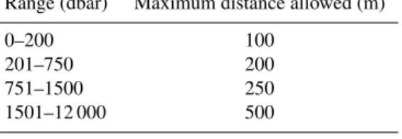
Table 1.Maximum distance criteria used when vertically interpolating the input data.

Range (dbar) Maximum distance allowed (m)

0–200 100

201–750 200

751–1500 250

1501–12 000 500

into the mapping procedure was found to improve the result – often specifically because of their remoteness from other cruises

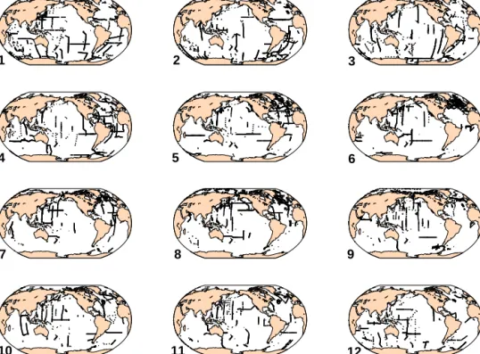
Open-ocean biogeochemical measurements tend to have a seasonal bias at high latitudes because of prohibitive winter- time weather. Figure 1 shows the data distribution in G16D in each month of the year. The seasonal bias is clear: the North Atlantic is almost exclusively sampled in May–August (boreal summer); the Southern Ocean is almost exclusively sampled in December–March (austral summer); the eastern North Pacific has significant amounts of data only in June, August, and September; the tropical Atlantic Ocean has a January–April bias; and the only region with a reasonably full annual data coverage is the western North Pacific. No at- tempt has been made to correct for a possible seasonal bias in the mapped climatologies. Due to the limited data coverage, such corrections would have to rely on relationships with ancillary variables and different temporal gap-filling methods.

This is an endeavor in itself and something that may be at- tempted for future versions of GLODAP but would also increase the errors and uncertainties in the mapped climatologies. We therefore concede that the G16M data product as presented here is for many regions more representative of summertime mean conditions than annual mean conditions, and users should take this into account when using the data product.

The following pre-mapping data treatments were carried out on the data of G16D:

1. The original cruise data were quality-controlled using a crossover and inversion method, which entails identify- ing biases between stations within a fixed distance and then evaluating all biases for all cruises to determine the corrections necessary to make all cruises consistent. The details of the quality control process are given in Olsen et al. (2016).

2. All bias-minimized data were vertically interpolated onto 33 surfaces: 0, 10, 20, 30, 50, 75, 100, 125, 150, 200, 250, 300, 400, 500, 600, 700, 800, 900, 1000, 1100, 1200, 1300, 1400, 1500, 1750, 2000, 2500, 3000, 3500, 4000, 4500, 5000, and 5500 m. These depths are the same as those used in GLODAPv1.1 and originally chosen by Levitus and Boyer (1994). The interpolation was done station by station, using a cubic hermite spline

function. This interpolation method is generally robust, but it can give unreliable results in a few unusual cir- cumstances, especially near the surface. Consequently, if this interpolation gave values more than 1 % different from those produced using a simple linear vertical interpolation, the linear results were used. We used the maximum distance criteria specified in Table 1 to avoid interpolation over excessive vertical distances between data points. These maximum distance criteria are the same as those used by Key et al. (2004) for GLODAPv1.1.

3. The vertically interpolated data for each depth surface were then gridded by bin-averaging all data in each 1^◦×1^◦ grid cell. The mapped climatologies are thus based on gridded (or “bin-averaged”) data, not individual measurements. We do this because the repeat hydrography program yielded several transects in the ocean that may have differing observations at nearly exactly the same location, which in frontal regions may otherwise have deleterious effects on the results of mapping.

4. G16D includes data for the period 1972–2013, during which the atmospheric levels of CO₂increased strongly.

Consequently, within this time frame, oceanic TCO₂ and related properties (e.g., pH and the saturation states of CaCO₃) have seen strong increases, particularly at shallower levels (e.g., Orr et al., 2001; Lauvset et al., 2015; Sabine and Tanhua, 2010). To correct for this, all TCO2data in G16D were normalized to the year 2002 prior to mapping. The details of this procedure are given in Appendix B. The employed methodology likely has substantial uncertainty, partially due to (local) invalidity of assumptions and its practical implementation. Nev- ertheless, for the purpose of creating a global mapped climatology of TCO₂ for G16M this uncertainty was deemed necessary in order to reduce the risk of convert- ing time trends into spatial variations. Being able to use all 42 years of observations in the mapping significantly reduces the mapping error.

5. _Cand_Awere calculated from the TCO²⁰⁰²₂ and TAlk pair at in situ temperature and pressure, while pH was calculated from the TCO²⁰⁰²₂ and TAlk pair at both in situ temperature and pressure and at constant temperature (25^◦C) and pressure (0 dbar). All calculations were performed using the MATLAB version (van Heuven et al., 2009) of CO₂SYS (Lewis and Wallace, 1998). We used pressure, temperature, salinity, phosphate, and silicate from G16D; the dissociation constants of Lueker et al. (2000) for carbonate, and those of Dickson (1990) for sulfate; and the total borate–salinity relationship of Uppström (1974).

(4)

1 2 3

4 5 6

7 8 9

10 11 12

Figure 1.Monthly data density of TCO₂in the years 1972–2013. The figure includes all data shallower than 150 m.

2.2 Derived variables

In G16M we provide mapped climatologies of both anthropogenic carbon (C_ant) and preindustrial carbon (TCO^preind₂ ).

These are based on using a classical application of the tran- sit time distribution (TTD) method (e.g., Hall et al., 2002;

Waugh et al., 2006) on all available CFC-12 data in G16D.

Users of these fields should be aware that they were ob- tained by a relatively crude application of the TTD methodology, and that both rely on first-order approximations and assumptions (Appendix B). However, the TTD methodology followed is not different from, for example, that used by Waugh et al. (2006) based on GLODAPv1.1 and may, due to the higher data coverage and quality in G16D, be considered an improvement of that earlier work. Subtracting C_ant from TCO2provides TCO^preind₂ , which is of considerable rel- evance to ocean biogeochemical modeling studies and thus also mapped and included in the G16M data product.

2.3 Mapping method

The Data-Interpolating Variational Analysis (DIVA) mapping method (Beckers et al., 2014; Troupin et al., 2012) was used to create the mapped climatologies. DIVA is the implementation of the variational inverse method (VIM) of mapping discrete, spatially varying data. A major difference between this and the optimal interpolation (OI) method used in GLODAPv1.1 is how topography is handled. DIVA takes the presence of the seabed and land into account during the

mapping and gives better results in coastal areas and around islands. In addition, the entire global ocean can be mapped at once, for example, DIVA does not propagate information across narrow land barriers such as the Panama isthmus.

Consequently, there is no need to split the data into ocean regions which then must be stitched together to form a global map (like in, for example, GLODAPv1.1; Key et al., 2004), or to apply basin identifiers which tell the software where to exclude nearby data because they are on the other side of a topographical feature (like in, for example, World Ocean At- las, Locarnini et al., 2013). In DIVA the topography is used to generate a finite-element mesh inside the topography contour on a given depth surface and the cost function DIVA uses to create an analysis field (see below) is then solved for each triangle of the mesh. The mesh size is directly dependent on the correlation length scale (see below) in the open ocean, but near topography the mesh is also dependent on the shape of the topography contour. The analysis is then output on the specified regular grid. Eachgrid center pointhas to be inside a mesh triangle to be deemed “ocean”. Whether a cell at a given depth surface is masked as land or not is therefore a result of the choice of topography and the detail of the finite-element mesh.

Apart from the data, the most important DIVA input parameters are the spatial correlation length scale (CL) and the data signal-to-noise ratio (SNR). The CL defines the charac- teristic distance over which a data point influences its neigh- bors. For G16M.2016 this was defined a priori as 7^◦for all parameters. Since the oceans generally tend to mix more eas-

(5)

ily zonally than meridionally, a scaling factor was used to make the east–west correlation length twice the defined input (see the DIVA user manual available at http://modb.oce.

ulg.ac.be/mediawiki/index.php/Diva_documents for details).

These settings give zonal and meridional correlation length scales that closely match those used for GLODAPv1.1, but this implies having to use Cartesian coordinates. Note that setting the CL is partly a subjective effort, aiming to strike the optimal balance between large values that tend to smooth the data fields and reduce mapping errors and small values that lead to more correct rendering of fronts and other features. We also want to stay within the physical constraints set by ocean dynamics and natural spatial variability. It is possible to locally optimize CL in DIVA, but this works well only when the data density is reasonably high. The sparse global data distribution in G16D gives optimized CL in the order of 25^◦. Doing a cruise-by-cruise analysis following Jones et al. (2012) to get spatially varying CL is possible, but this would leave large gaps where we would have to guess CL.

For G16M it was therefore decided to use a globally uniform a priori value since this is the most transparent and repro- ducible.

The SNR defines how representative the observations are for the climatological state. For spatially varying data sets like G16D, it is the assumed ratio of climatological spatial variability (“signal”) to the short-term variability (“noise”) in the data. For G16M the SNR was defined a priori to be 10 (i.e., the noise is 10 % of the signal), following Key et al. (2004). To understand the importance of SNR, and the reason for a subjective a priori choice, a brief discus- sion of the differences between interpolation and approximation/analysis is necessary. When interpolating between points in a data set, gaps between data points are filled but the existing points are not replaced. Whenapproximating, a function (e.g., a regression line) is applied that describes the original data points to some degree. The resulting approximated data set has new values at every point and is smoother than the interpolated data set. None of the approximated data points exactly match the original ones. That assumes more uncertainty – or non-climatological variability – in the data.

In the case of very high SNR, the observed values are re- tained in the mapped climatology and DIVA interpolates between them, while smaller values allow for larger deviations from these and an increasingly smooth climatology.

Working with real-world observations, we know that the observations are indeed affected by shorter-term variations and in addition have analytical uncertainties associated with them. They do not represent the “true” climatological value.

For this reason the SNR should always be kept quite small when making mapped climatologies, but this needs to be bal- anced by the need to keep the error estimates reasonable. The lower the SNR the further the approximation is allowed to deviate from the original data and the higher the error associated with the approximation becomes. The SNR can be calculated from observations using generalized cross valida-

tion, but for G16D such calculations give very high SNR (in the order of 100). This is maybe not completely unreason- able, since G16D has been carefully quality-controlled and we have high confidence that the measurement uncertainties are small. However, both increasing the SNR and increasing the CL will decrease the error estimates, because this assumes small representativity errors (i.e., that what is observed is the true climatology) and a large circle of influence. We know that there is a seasonal bias in the observations which therefore do not represent the true climatological values, and if the assumptions above are wrong the errors will be significantly underestimated. Therefore, the mapping errors are likely to be underestimated if we use the SNR calculated from general cross validation.

A DIVA analysis is created by minimizing a cost function which is defined by the difference between observations and analysis, the smoothness of the analysis, and the physical laws of the ocean (Troupin et al., 2012). The result is thus the analysis with the smallest global mean error, but deter- mining the spatial distribution of errors is important as well.

In DIVA this is non-trivial as, in contrast to OI, the real covariance function, which is necessary to obtain spatial error fields, is not formulated explicitly but is instead the result of a numerical determination (Troupin et al., 2012). Determin- ing the real covariance to get error estimates is the most exact method, but it is computationally expensive. There are several error estimation methods implemented in DIVA, from the very simple to the very exact (Troupin et al., 2012; Beck- ers et al., 2014). Due to computational cost, for G16M the error fields are based on the “clever poor man’s error calculation”. A detailed description of this method is given in Beck- ers et al. (2014). Based on detailed studies of the Mediter- ranean Sea, Beckers et al. (2014) estimate that this method underestimates the real error by∼25 %. The underestima- tion is not uniform, though, and larger in areas with high data density, while in areas where observational data are more than one CL distant, the clever poor man’s error represents the true error well (Beckers et al., 2014). The error fields are thus appropriate to determine where the error is too large for the user’s planned use of the mapped climatologies.

2.4 Output and post-processing

Each of the G16M climatologies are global analyses for the range−180 to 180^◦E with a 1^◦×1^◦spatial resolution and 33 vertical layers, performed on a Cartesian coordinate system from−340 to 20^◦E. To ensure that the analyses con- verges on the analysis boundary at 20^◦E the input data (i.e., the observations) were duplicated for 10^◦ on either side of 20^◦E before mapping. This duplication is a combination of (i) mirroring the observations for 2^◦ on either side of 20^◦E, (ii) copying the observations in the area 10–20^◦E to 15–25^◦E and to 20–30^◦E, and (iii) copying the observations in the area 20–30^◦E to 15–25^◦E and to 10–20^◦E.

This is necessary mostly due to the paucity of data along the

(6)

boundary. The topography file has a longitudinal distance of 400^◦ to ensure that the analysis neither begins nor ends at the end of the finite-element triangular mesh. In addition, a weighted average over 10^◦ on either side of the boundary was used to smooth the analysis in post-processing. This re- moves most discontinuities along these boundaries. Where discontinuities are still visible, they are not significant (i.e., not greater than the mapping uncertainty). The topography is a priori known by DIVA, so no land masks need be applied in post-processing. However, other masks have been applied:

1. A mask removing the results in all grid cells where the relative mapping error exceeds 0.75 was applied. This mask effectively masks closed regions with no observational data, in addition to masking regions where the DIVA analysis is considered too uncertain to be useful.

2. Masks covering the Red Sea, Gulf of Mexico, Caribbean Sea, and parts of the Canadian Archipelago were applied. In these regions the mapping error is not overly large relative to the standard deviation in the global data, but a general lack of data and our knowledge of oceanographic features lead to the conclusion that the mapped climatologies do not appropriately re- flect the real world in these regions.

3. In the Arctic Ocean, cells where the DIVA analysis results in values that differ from the observational mean in the different basins by more than 2.5 % were masked.

Further details regarding the Arctic Ocean are given in Sect. 2.5.

2.5 Mapping the Arctic Ocean

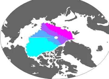
Mapping data in the Arctic Ocean is challenging for several reasons: (i) our choice to increase the zonal correlation length (relative to the meridional CL) required us to work with an equidistant world which is very inappropriate for the high- latitudes; (ii) the Arctic Ocean contains the northern boundary of DIVA’s (Cartesian) finite-element mesh, which causes peculiar artifacts; and (iii) there is a limited amount of observations. The combination of these three factors can lead to unrealistic results for the Arctic. We found that the DIVA analysis yields useful results in the top 1000 m of the Arctic Ocean. However, we have applied an additional mask based on deviation from the observational averages to remove spurious boundary effects (Sect. 2.4). Deeper than 1000 m, however, DIVA is not able to provide useful climatological fields in the Arctic Ocean. It has therefore been decided to replace the DIVA analysis with the basin averages for each depth surface below 1000 m (i.e., surfaces 20–33). For these surfaces the mapping error has been replaced with the standard deviation of this average. The boundaries we have used for the four basins in the Arctic Ocean are shown in Fig. 2.

Figure 2.Map of the Arctic Ocean with the four basins’ definitions used to calculate averages shown in different colors.

3 Results

3.1 Data fields

The mapped climatologies are available from CDIAC (http:

//cdiac.ornl.gov/oceans/GLODAPv2/) as one folder named GLODAPv2.2016b_Mapped_Climatology. This folder contains netCDF files for each parameter. Each of these netCDF files contain the global 1^◦×1^◦climatology of a parameter, the associated error field, and the gridded input data for the parameter in question (Table 2).

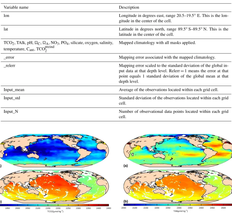
Figures 3–5 show the mapped climatologies for TCO₂, TAlk, and nitrate, respectively, at two different depth surfaces. These all show the spatial patterns expected from biological dynamics, evaporative processes, and large-scale cir- culation: higher values of each in the deep Pacific Ocean than in the deep Atlantic Ocean illustrate the greater age of water in the deep Pacific Ocean; a higher concentration of reminer- alized carbon and nutrients at depth than at the surface; and higher surface ocean TAlk in the subtropics, where salinity is highest. The rather low nitrate at the surface highlights the summer bias in the climatologies, except in the South- ern Ocean, where the biological production does not fully utilize available nutrients and where there is both upwelling and strong vertical mixing. Figures 6–8 show, for the same parameters and depth surfaces, the difference between the gridded input and the mapped climatologies, which is relatively large and variable near the surface and generally within the data uncertainties in the deep ocean. Figures 9–11 show the error fields associated with the climatologies shown in Figs. 3–5.

3.2 Error fields

While the mapping error reflects the data distribution and the choice of input variables (i.e., CL and SNR), it represents

(7)

Table 2.List of information available in the netCDF data files.

Variable name Description

lon Longitude in degrees east, range 20.5–19.5^◦E. This is the lon-

gitude in the center of the cell.

lat Latitude in degrees north, range 89.5^◦S–89.5^◦N. This is the

latitude in the center of the cell.

TCO₂, TAlk, pH,_C,_A, NO₃, PO₄, silicate, oxygen, salinity, temperature, C_ant, TCO^preind₂

Mapped climatology with all masks applied.

_error Mapping error associated with the mapped climatology.

_relerr Mapping error scaled to the standard deviation of the global in-

put data at that depth level. Relerr=1 means the error at that point equals 1 standard deviation of the global mean at that depth level.

Input_mean Average of the observations located within each grid cell.

Input_std Standard deviation of the observations located within each grid

cell.

Input_N Number of observational data points located within each grid

cell.

(a)

(b)

TCO2(μmol kg⁻¹)

1900 1950 2000 2050 2100 2150 2200 2250 2300 2350 2400 2450

Figure 3.Mapped climatology of TCO₂at 10 m(a)and 3000 m(b).

only the errors due to the mathematical mapping of the input data, and does not take into account all the uncertainty in the input data (although some of this uncertainty is accounted for in the choice of SNR). The error fields moreover do not include calculation errors for those variables that are calculated from other measurements (e.g., pH and CaCO₃saturation states). For details regarding the accuracy and precision of the G16D data product the reader is referred to Olsen et al. (2016); briefly, the uncertainties in the input data overall are smaller than the mapping errors. Overall, the spatial error distribution is as expected: relatively small where there are observations and larger elsewhere. All grid cells where therelativemapping error (i.e., the ratio of the absolute map-

(a)

(b)

TAlk(μmol kg⁻¹)

2050 2100 2150 2200 2250 2300 2350 2400 2450 2500 2550

Figure 4.Mapped climatology of TAlk at 10 m(a)and 3000 m(b).

ping error at a grid point over the standard deviation of all the data on that depth level) exceeds 0.75 have been masked.

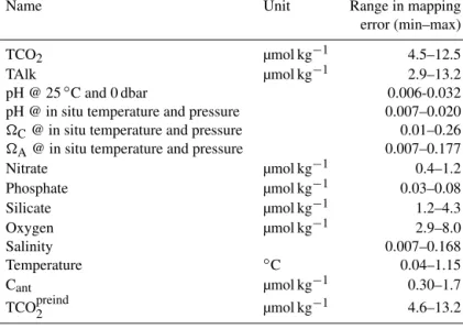
This step nonetheless leaves several regions with highabso- lutemapping errors. The relative error fields are provided in the netCDF files, making it possible for the user to create alternative masks if desired. The range from minimum to maximum error for the different parameters (Table 3) reflects the variability in data values and data density on different surfaces. The spatial variability in the mapping errors in large part depends on the layout of the observational network, and further study of this variability would be of great use in opti- mizing existing and future observational networks.

(8)

Table 3.Table of the range in mapping error averaged spatially over all depth surfaces for the individual parameters.

Name Unit Range in mapping

error (min–max)

TCO₂ µmol kg⁻¹ 4.5–12.5

TAlk µmol kg⁻¹ 2.9–13.2

pH @ 25^◦C and 0 dbar 0.006-0.032

pH @ in situ temperature and pressure 0.007–0.020

_C@ in situ temperature and pressure 0.01–0.26

_A@ in situ temperature and pressure 0.007–0.177

Nitrate µmol kg⁻¹ 0.4–1.2

Phosphate µmol kg⁻¹ 0.03–0.08

Silicate µmol kg⁻¹ 1.2–4.3

Oxygen µmol kg⁻¹ 2.9–8.0

Salinity 0.007–0.168

Temperature ^◦C 0.04–1.15

Cant µmol kg⁻¹ 0.30–1.7

TCO^preind₂ µmol kg⁻¹ 4.6–13.2

(a)

(b)

NO3(μmol kg⁻¹)

0 5 10 15 20 25 30 35 40

Figure 5. Mapped climatology of nitrate at 10 m (a) and 3000 m(b).

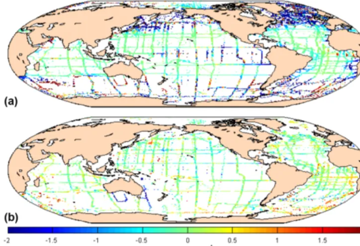
The mapping errors for TCO₂ and TAlk in G16M have been compared with those of GLODAPv1.1 (Figs. 12–13).

Differences are expected from the different methods used to calculate the errors and do not necessarily indicate one product to be of superior quality. The most obvious result is the large spatial variability in the differences, particularly at depth, which seem to correlate with the data distribution.

Very generally, there are large differences (∼10 µmol kg⁻¹) in error estimates between G16M and GLODAPv1.1 for both TCO₂ (Fig. 12) and TAlk (Fig. 13) in the top 200 m of the Southern Ocean (exemplified by the 10 m surface in Figs. 12a and 13a). In this case the error estimate of both TCO₂and TAlk in G16M is frequently 15 µmol kg⁻¹higher than in GLODAPv1.1. For the rest of the world, however, the G16M errors are smaller than the GLODAPv1.1 errors for both TCO₂and TAlk. Below 1000 m (exemplified by the

Figure 6.Difference between the gridded TCO₂input data and the mapped climatologies at 10 m(a)and 3000 m(b).

3000 m surface in Figs. 12b and 13b) the mapping errors are globally larger by 0–10 µmol kg⁻¹ in G16M than in GLO- DAPv1.1. Generally, for the deep ocean the error difference is greatest in the Pacific and Southern oceans, while the At- lantic Ocean is relatively comparable (Figs. 12b and 13b). A more comprehensive study of the differences in mapping error between GLODAPv1.1 and G16M and the mechanisms behind these would be worthwhile, and may improve future climatologies of the marine CO₂chemistry, but is beyond the scope of this paper. The exact reasons for the differences seen in Figs. 12–13 are currently not evident, but several things are likely to contribute: (i) differences in the methods used, and particularly that the method used by G16M is known to underestimate the real errors by as much as 25 %, and (ii) there are differences in data density and data distribution, with the improved distribution in G16D revealing more small-scale

(9)

Figure 7.Difference between the gridded TAlk input data and the mapped climatologies at 10 m(a)and 3000 m(b).

Figure 8.Difference between the gridded nitrate input data and the mapped climatologies at 10 m(a)and 3000 m(b).

natural variability and thus larger, more realistic, mapping errors.

For the macronutrients (nitrate, phosphate, silicate) G16M can be compared to the World Ocean Atlas 2009 (WOA09) nutrient climatologies (Garcia et al., 2010). Before doing so several things need to be considered: (i) methods used for mapping WOA09 (Garcia et al., 2010) are very different from those used in G16M and (ii) WOA09 does not provide mapped error estimates for their climatologies (only the difference in the 1^◦×1^◦cells with observations), precluding a direct comparison of errors. Instead, we compare G16M with WOA09 by plotting the difference between (i) the annual NO₃climatology of WOA09 and (ii) the bin-averaged data of G16M. For the purpose of this comparison we roughly con- verted the WOA09 data from µmol L⁻¹to µmol kg⁻¹by di- viding by 1.024. Differences will be due to a combination of the differences in input data and the differences in mapping methods and the comparison reveals that at 10 m depth the

(a)

(b)

TCO2(μmol kg⁻¹)

0 10 20 30 40 50 60

Figure 9.Mapping error for TCO₂ at 10 m(a)and 3000 m(b).

Notice how the error increases with distance from transects, creating a spatial pattern of square-like features in the Pacific.

(a)

(b)

TAlk(μmol kg⁻¹)

0 10 20 30 40 50 60

Figure 10.Mapping error for TAlk at 10 m(a)and 3000 m(b).

G16M bin-averaged observations are generally lower than the WOA09 climatology in high latitudes (Fig. 14a). This is most likely a manifestation of the summertime bias in GLO- DAPv2 observations. In the tropics and subtropics the differences are within the data and mapping uncertainties. In the deep ocean (Fig. 14b) the differences between the G16M bin- averaged observations and WOA09 are occasionally quite pronounced (for instance in the southeastern Atlantic Ocean, and south and southeast of Australia, where G16D performed significant adjustments to some cruises). However, in general, the match between GLODAPv2 and WOA09 at depth is encouraging. This suggests that, below the seasonally influ- enced surfaces, the differences between G16M and WOA09 stem mainly from differences in mapping method and input data but that the climatologies otherwise are comparable. The biggest difference between G16M and WOA09 is that the lat-

(10)

Figure 11.Mapping error for nitrate at 10 m(a)and 3000 m(b).

Figure 12. Mapping error for TCO₂ in GLODAPv2.2016b mi- nus mapping error for TCO₂ in GLODAPv1.1 at 10 m (a)and 3000 m(b). Note that the differences are mainly attributable to differences in method and not real reductions/increases in mapping error.

ter has considerably more input data and is thus able to provide monthly climatologies. We have compared the G16M nitrate climatology to the WOA09 nitrate climatology since the more recent WOA13 has a very different vertical resolution of 137 surfaces (Locarnini et al., 2013), compared to 33 in G16M.

We note that there is a significant difference in total ocean volume between G16M and WOA09, with WOA09 having a 10 % larger volume than G16M. This difference likely comes from differences in how topography is handled in the two methods used and, related to that, the application of land masks, but the exact details of how and where these differences occur are beyond the scope of this paper.

Figure 13. Mapping error for TAlk in GLODAPv2.2016b mi- nus mapping error for TAlk in GLODAPv1.1 at 10 m (a) and 3000 m(b). Note that the differences are mainly attributable to differences in method and not real reductions/increases in mapping error.

Figure 14. GLODAPv2.2016b nitrate gridded input data mi- nus WOA09 annual mapped nitrate climatology at 10 m(a) and 3000 m(b).

4 Notes on the nutrient and oxygen fields of GLODAPv2.2016b

For G16M we have mapped (among other parameters) macronutrients, oxygen, salinity, and temperature. For each of these parameters, the World Ocean Atlas already provides climatologies based on substantially more data (additionally yielding monthly and seasonal climatologies). The reason the mapped climatologies of macronutrients, oxygen, salinity, and temperature are made available as a part of G16M is that we see value in having such fields created using the same method as the CO₂chemistry parameters. A result thereof is that the provided fields are more compatible for common application: (i) the error fields are calculated using the same method, (ii) the strengths and weaknesses of the method are

(11)

the same, and (iii) the quality control and data treatment (e.g., vertical interpolation, gridding) are the same. Thus, if the intent of a user is to study nutrient dynamics, or even validate nutrient fields from models, the WOA fields are likely to be the best choice, but if the intent is to analyze nutrients and physics in relation to spatial variability of the ocean CO₂ chemistry, then the G16M data product is appropriate, and likely even preferred. For studies of ocean CO₂ chemistry having the nutrients and physical variables mapped with the exact same method should prove to be both useful and con- venient.

5 Future work

Several updates and additions are planned or underway. This future work includes mapping of several additional parameters that may be derived from in the G16D data product, such as water ages based on the halogenated transient tracer data and the¹⁴C data. Also, a more advanced TTD-based calculation of anthropogenic carbon (e.g., with spatially varying 0/1) is planned and will be described in separate papers.

Additionally, a future update may fill the cells that intersect with bottom topography and will come with a field of bottom depths for each 1^◦×1^◦water column so that more accurate column inventories can be produced. It has been suggested to create mapped climatologies on density surfaces rather than standard depths. This will be considered, but given that DIVA needs the topography as an a priori input, a new topography file needs to be carefully created. Any such new additions to G16M (or to future versions thereof) will be described in separate, independent papers.

6 Data availability

For information on how to download the described data please see Sect. 3.1.

(12)

Appendix A: A note on naming

GLODAP will be added to and updated with new major cruises on a regular basis and the updated versions of the data product will be named GLODAPv2.yyyy, where yyyy is the given year in which the update takes place. For these updates new cruises will be quality-controlled using the quality control routines of Lauvset and Tanhua (2015) or similar, under the assumption that GLODAPv2.2016 represents

“ground truth”. Every decade or so, following the timing of major ocean-wide observational plans like GO-SHIP, a complete remake is planned and all cruises will be quality- controlled using the cross-over and inversion routines described in Olsen et al. (2016). These remakes of GLODAP will get new integer appendices (v3, v4, etc.). Following this system, the current GLODAP data product – both the discrete bias-corrected data product and the mapped climatologies (both available at CDIAC) – would be named GLODAPv2.2016. However, the improvements to the initial mapped climatologies as resulting from the peer-review process have resulted in an updated version for the current year, named GLODAPv2.2016b.

Differences between the GLODAPv2.2016 and GLODAPv2.2016b mapped climatologies

During the review process of the earlier GLODAPv2.2016 mapped climatologies, several improvements were made, based in part on suggestions by reviewers. The thus improved mapped product is the one discussed in this paper. The differences are as follows:

– An error in the GLODAPv2.2016 grid is now fixed so that the fields align with the world topography and the grid is the same as that in GLODAPv1.1 and WOA.

– The latitudinal boundary of the mapping domain was moved from 180 to 20^◦E to minimize the effect of any boundary effects during mapping.

– An additional smoothing across this boundary is added in post-processing.

– The scheme for handling coordinate system transfor- mation and scaling of the correlation length scale has changed. This means that for GLODAPv2.2016b we no longer used an advection constraint to ensure stronger correlation zonally but instead manipulate the coordinate system to scale the zonal CL to 2 times the meridional CL. Implicitly this means that every cell on the grid is equidistant, and this leads to some spurious effects at very high latitudes (poleward of∼75^◦).

– For the Arctic Ocean, because of its closeness to the northern boundary and the spurious effects encountered with the equidistant grid, we have applied an additional

mask to remove boundary effects and used alternative methods at depths greater than 1000 m (see Sect. 2.5).

– Due to time constraints, the “almost exact” error calculation has been replaced by the “clever poor man’s”

error calculation. Based on detailed studies of the Mediterranean Sea (Beckers et al., 2014) the latter tends to underestimate the error by∼25 % compared to the real covariance (“true”) error calculation. The underesti- mation is not uniform, though, and much larger in areas with high data density. In areas where observational data are more than one CL distant, the clever poor man’s error represents the true error well (Beckers et al., 2014).

– We have manually masked some ocean regions where the errors are quite small but where we, based on our knowledge of spatial gradients and patterns of the ocean CO₂ parameters, do not trust the results of the DIVA analysis. These areas include the Red Sea, the Gulf of Mexico, the Caribbean Sea, and parts of the Canadian Archipelago. There are also a very limited number of observations available in these regions.

– GLODAPv2.2016b contains two additional parameters:

Cantand TCO^preind₂ .

Appendix B: Procedure followed for normalization of TCO₂data to the year 2002

For the purpose of normalizing the G16D TCO₂data to the year 2002, we consider TCO₂ to consist of a “natural” or

“preindustrial” and an anthropogenic component (Eq. B1), and normalize C_antto 2002:

TCO₂=TCO₂^preind+C_ant. (B1)

We infer C_ant using a classical application of the tran- sit time distribution (TTD) method (e.g., Hall et al., 2002;

Waugh et al., 2006) on all available CFC-12 data in G16D, under the assumption of mean age and age distribution width being equal (i.e.,0/1=1). Subsequently, we employ a normalization following the “atmospheric perturbation” concept proposed by Ríos et al. (2012). Herein, under the assumption of transient steady state (TSS; Tanhua et al., 2007), one re- lates the accumulation of Cant in an ocean sample with the accumulation of Cantin the atmosphere, allowing scalability to other future or past pCO2, as long as the atmospheric perturbation progresses at an approximately exponential fash- ion. Thus, with knowledge of the time history of atmospheric anthropogenic CO₂perturbation (i.e.,pCO^atm₂ −280), we infer for every ocean sample its sensitivity “S” (Eq. B2) to the atmospheric perturbation (with units of µmol kg⁻¹µatm⁻¹).

S=C^TTD_ant ^T/(pCO^atm₂ ^T −280) (B2) This ratio is high at the surface, while it approaches zero at depth and is higher in the tropics than in (sub)polar regions. Tropical surface water values for S are found to

(13)

be 0.7±0.1 µmol kg⁻¹µatm⁻¹, while subpolar values are 0.4±0.1 µmol kg⁻¹µatm⁻¹, fully consistent with thermody- namic expectations. Values should not change much over time at any given location, meaning that estimates of S from the 1980s should resemble those from the 2010s for a given water sample. In practice, however, both values decrease slightly over time, consistent with the expected pro- gressing “ocean saturation” at higher C_ant, precluding use of the methodology over arbitrarily long data records. However, over the approximately 40 years spanned by G16D, this decrease does not meaningfully affect our application.

For samples with a valid TCO2 value, but for which S could not be calculated due to lack of an accompanying CFC- 12 measurement, we used the averageSof surrounding samples, assuming values ofS to be generally representative of the ocean layer where they were determined. Search extent was limited in vertical direction to approximately±15 % of the sample depth to prevent inclusion of results for S from very different ventilation layers. Horizontal limits to search

box extent (edge lengths of 6^◦ in latitude and 12^◦ in longitude, expanding stepwise to 10^◦×20^◦ for very isolated samples) prevented some highly spatially isolated samples from getting a value ofSassigned. Nonetheless, we inferred C^TTD_ant ²⁰⁰² for 367 522 of 367 886 (99.99 %) of samples that have measured TCO₂, while only 75 % of those have measured CFC-12.

Subsequently, for every sample we normalize TCO2to the year 2002 using Eq. (B3):

TCO2,2002=TCO2,T −S×(pCO^atm₂ ^T−pCO^atm₂ ²⁰⁰²). (B3) As a last step, we similarly produce quasi-synoptic values of C_ant following Eq. (B4), and with this an estimate of TCO^preind₂ .

C^TTD_ant ²⁰⁰²=C^TTD_ant ^T −S×(pCO₂^atm_T −pCO₂^atm²⁰⁰²) (B4)

(14)

Acknowledgements. The work of S. K. Lauvset was funded by the Norwegian Research Council through the projects DECApH (214513/F20). The EU-IP CARBOCHANGE (FP7 264878) project provided funding for A. Olsen, S. van Heuven, T. Tanhua, R. Ste- infeldt, and M. Hoppema and is the project framework that in- stigated GLODAPv2. A. Olsen additionally acknowledges gener- ous support from the FRAM – High North Research Centre for Climate and the Environment, the Centre for Climate Dynamics at the Bjerknes Centre for Climate Research, the EU AtlantOS (grant agreement no. 633211) project, and the Norwegian Research Council project SNACS (229752). Emil Jeansson appreciates support from the Norwegian Research Council project VENTILATE (229791). R. Key was supported by KeyCrafts grant 2012-001, CICS grants NA08OAR4320752 and NA14OAR4320106, NASA grant NNX12AQ22G, NSF grants OCE-0825163 (with a supple- ment via WHOI P.O. C119245) and PLR-1425989, and Battelle contract #4000133565 to CDIAC. A. Kozyr acknowledges funding from the US Department of Energy. M. Ishii acknowledges the project MEXT 24121003. A. Velo and F. F. Pérez were supported by the BOCATS (CTM20134410484P) project cofounded by the Spanish government and the Fondo Europeo de Desarrollo Regional (FEDER). The International Ocean Carbon Coordination Project (IOCCP) partially supported this activity through the U.S.

National Science Foundation grant (OCE- 1243377) to the Scien- tific Committee on Oceanic Research.

The research leading to the last developments of DIVA has received funding from the European Union Seventh Framework Programme (FP7/2007-2013) under grant agreement no. 283607, SeaDataNet 2, and from the project EMODNET (MARE/2012/10 – Lot 4 Chemistry – SI2.656742) from the Directorate-General for Maritime Affairs and Fisheries.

Edited by: G. M. R. Manzella Reviewed by: two anonymous referees

References

Bakker, D. C. E., Pfeil, B., Smith, K., Hankin, S., Olsen, A., Alin, S. R., Cosca, C., Harasawa, S., Kozyr, A., Nojiri, Y., O’Brien, K. M., Schuster, U., Telszewski, M., Tilbrook, B., Wada, C., Akl, J., Barbero, L., Bates, N. R., Boutin, J., Bozec, Y., Cai, W.-J., Castle, R. D., Chavez, F. P., Chen, L., Chierici, M., Cur- rie, K., de Baar, H. J. W., Evans, W., Feely, R. A., Fransson, A., Gao, Z., Hales, B., Hardman-Mountford, N. J., Hoppema, M., Huang, W.-J., Hunt, C. W., Huss, B., Ichikawa, T., Johan- nessen, T., Jones, E. M., Jones, S. D., Jutterström, S., Kitidis, V., Körtzinger, A., Landschützer, P., Lauvset, S. K., Lefèvre, N., Manke, A. B., Mathis, J. T., Merlivat, L., Metzl, N., Murata, A., Newberger, T., Omar, A. M., Ono, T., Park, G.-H., Pater- son, K., Pierrot, D., Ríos, A. F., Sabine, C. L., Saito, S., Salis- bury, J., Sarma, V. V. S. S., Schlitzer, R., Sieger, R., Skjelvan, I., Steinhoff, T., Sullivan, K. F., Sun, H., Sutton, A. J., Suzuki, T., Sweeney, C., Takahashi, T., Tjiputra, J., Tsurushima, N., van Heuven, S. M. A. C., Vandemark, D., Vlahos, P., Wallace, D. W.

R., Wanninkhof, R., and Watson, A. J.: An update to the Surface Ocean CO₂Atlas (SOCAT version 2), Earth Syst. Sci. Data, 6, 69–90, doi:10.5194/essd-6-69-2014, 2014.

Beckers, J.-M., Barth, A., Troupin, C., and Alvera-Azcárate, A.: Approximate and Efficient Methods to Assess Error

Fields in Spatial Gridding with Data Interpolating Varia- tional Analysis (DIVA), J. Atmos. Ocean. Tech., 31, 515–530, doi:10.1175/JTECH-D-13-00130.1, 2014.

Bopp, L., Resplandy, L., Orr, J. C., Doney, S. C., Dunne, J. P., Gehlen, M., Halloran, P., Heinze, C., Ilyina, T., Séférian, R., Tjiputra, J., and Vichi, M.: Multiple stressors of ocean ecosys- tems in the 21st century: projections with CMIP5 models, Biogeosciences, 10, 6225–6245, doi:10.5194/bg-10-6225-2013, 2013.

Dickson, A.: Standard potential of the reaction: AgCl (s) + 1/2H2(g)=Ag (s)+HCl (aq), and the standard acidity constant of the ion HSO⁻4 in synthetic sea water from 273.15 to 318.15 K, J. Chem. Thermodyn., 22, 113–127, doi:10.1016/0021- 9614(90)90074-z, 1990.

Feely, R., Talley, L., Bullister, J. L., Carlson, C. A., Doney, S., Fine, R. A., Firing, E., Gruber, N., Hansell, D. A., Johnson, G. C., Key, R., Langdon, C., Macdonald, A., Mathis, J., Mecking, S., Millero, F. J., Mordy, C., Sabine, C., Smethie, W. M., Swift, J.

H., Thurnherr, A. M., Wanninkhof, R., and Warner, M.: The US Repeat Hydrography CO₂/Tracer Program (GO-SHIP): Accom- plishments from the first decadal survey, US CLIVAR and OCB Report 2014-5, US CLIVAR Project Office, 47 pp., 2014.

Garcia, H. E., Locarnini, R. A., Boyer, T. P., Antonov, J. I., Zweng, M. M., Baranova, O. K., and Johnson, D. R.: World Ocean Atlas 2009, Volume 4: Nutrients (phosphate, nitrate, silicate), edited by: Levitus, S., NOAA Atlas NESDIS 71, U.S. Government Printing Office, Washington, DC, 398 pp., 2010.

Hall, T. M., Haine, T. W. N., and Waugh, D. W.: Inferring the concentration of anthropogenic carbon in the ocean from tracers, Global Biogeochem. Cy., 16, 1131, doi:10.1029/2001gb001835, 2002.

Jones, S. D., Le Quéré, C., and Rödenbeck, C.: Autocor- relation characteristics of surface ocean pCO₂ and air- sea CO₂ fluxes, Global Biogeochem. Cy., 26, GB2042, doi:10.1029/2010GB004017, 2012.

Key, R. M., Kozyr, A., Sabine, C. L., Lee, K., Wanninkhof, R., Bullister, J. L., Feely, R. A., Millero, F. J., Mordy, C., and Peng, T. H.: A global ocean carbon climatology: Results from Global Data Analysis Project (GLODAP), Global Biogeochem. Cy., 18, GB4031, doi:10.1029/2004GB002247, 2004.

Key, R. M., Tanhua, T., Olsen, A., Hoppema, M., Jutterström, S., Schirnick, C., van Heuven, S., Kozyr, A., Lin, X., Velo, A., Wal- lace, D. W. R., and Mintrop, L.: The CARINA data synthesis project: introduction and overview, Earth Syst. Sci. Data, 2, 105–

121, doi:10.5194/essd-2-105-2010, 2010.

Key, R. M., Olsen, A., van Heuven, S., Lauvset, S. K., Velo, A., Lin, X., Schirnick, C., Kozyr, A., Tanhua, T., Hoppema, M., Jutterström, S., Steinfeldt, R., Jeansson, E., Ishi, M., Perez, F. F., and Suzuki, T. Global Ocean Data Analysis Project, Version 2 (GLODAPv2), ORNL/CDIAC-162, NDP-P093. Car- bon Dioxide Information Analysis Center, Oak Ridge National Laboratory, US Department of Energy, Oak Ridge, Tennessee, doi:10.3334/CDIAC/OTG.NDP093_GLODAPv2, 2015.

Lauvset, S. K. and Tanhua, T.: A toolbox for secondary quality control on ocean chemistry and hydrographic data, Limnol.

Oceanogr. Meth., 13, 601–608, doi:10.1002/lom3.10050, 2015.

Lauvset, S. K., Gruber, N., Landschützer, P., Olsen, A., and Tjiputra, J.: Trends and drivers in global surface ocean pH over the past

(15)

3 decades, Biogeosciences, 12, 1285–1298, doi:10.5194/bg-12- 1285-2015, 2015.

Levitus, S. and Boyer, T. P.: World Ocean Atlas, vol. 4, Temper- ature, NOAA Atlas NESDIS 4, National Oceanic and Atmo- spheric Administration, Silver Spring, Md., 1994.

Lewis, E. and Wallace, D. W. R.: Program developed for CO₂ system calculations, in: ORNL/CDIAC-105, Carbon Diox- ide Information Analysis Center, Oak Ridge National Lab- oratory, U.S. Department of Energy, Oak Ridge, Tennessee, doi:doi:10.3334/CDIAC/OTG.PACIFICA_NDP092, 1998.

Locarnini, R. A., Mishonov, A. V., Antonov, J. I., Boyer, T. P., Gar- cia, H. E., Baranova, O. K., Zweng, M. M., Paver, C. R., Rea- gan, J. R., Johnson, D. R., Hamilton, M., and Seidov, D.: World Ocean Atlas 2013, Volume 1: Temperature, edited by: Levitus, S., Technical editor: Mishonov, A., NOAA Atlas NESDIS 73, 40 pp., 2013.

Lueker, T. J., Dickson, A. G., and Keeling, C. D.: Ocean pCO₂ calculated from dissolved inorganic carbon, alkalinity, and equa- tions for K-1 and K-2: validation based on laboratory measurements of CO₂in gas and seawater at equilibrium, Mar. Chem., 70, 105–119, doi:10.1016/s0304-4203(00)00022-0, 2000.

Olsen, A., Key, R. M., van Heuven, S., Lauvset, S. K., Velo, A., Lin, X., Schirnick, C., Kozyr, A., Tanhua, T., Hoppema, M., Jutterström, S., Steinfeldt, R., Jeansson, E., Ishii, M., Pérez, F.

F., and Suzuki, T.: The Global Ocean Data Analysis Project version 2 (GLODAPv2) – an internally consistent data product for the world ocean, Earth Syst. Sci. Data, 8, 297–323, doi:10.5194/essd-8-297-2016, 2016.

Orr, J. C., Maier-Reimer, E., Mikolajewicz, U., Monfray, P., Sarmiento, J. L., Toggweiler, J. R., Taylor, N. K., Palmer, J., Gru- ber, N., Sabine, C. L., Le Quéré, C., Key, R. M., and Boutin, J.: Estimates of anthropogenic carbon uptake from four three- dimensional global ocean models, Global Biogeochem. Cy., 15, 43–60, doi:10.1029/2000gb001273, 2001.

Pfeil, B., Olsen, A., Bakker, D. C. E., Hankin, S., Koyuk, H., Kozyr, A., Malczyk, J., Manke, A., Metzl, N., Sabine, C. L., Akl, J., Alin, S. R., Bates, N., Bellerby, R. G. J., Borges, A., Boutin, J., Brown, P. J., Cai, W.-J., Chavez, F. P., Chen, A., Cosca, C., Fassbender, A. J., Feely, R. A., González-Dávila, M., Goyet, C., Hales, B., Hardman-Mountford, N., Heinze, C., Hood, M., Hoppema, M., Hunt, C. W., Hydes, D., Ishii, M., Johannessen, T., Jones, S. D., Key, R. M., Körtzinger, A., Landschützer, P., Lauvset, S. K., Lefèvre, N., Lenton, A., Lourantou, A., Merlivat, L., Midorikawa, T., Mintrop, L., Miyazaki, C., Murata, A., Naka- date, A., Nakano, Y., Nakaoka, S., Nojiri, Y., Omar, A. M., Padin, X. A., Park, G.-H., Paterson, K., Perez, F. F., Pierrot, D., Poisson, A., Ríos, A. F., Santana-Casiano, J. M., Salisbury, J., Sarma, V. V.

S. S., Schlitzer, R., Schneider, B., Schuster, U., Sieger, R., Skjel- van, I., Steinhoff, T., Suzuki, T., Takahashi, T., Tedesco, K., Tel- szewski, M., Thomas, H., Tilbrook, B., Tjiputra, J., Vandemark, D., Veness, T., Wanninkhof, R., Watson, A. J., Weiss, R., Wong, C. S., and Yoshikawa-Inoue, H.: A uniform, quality controlled Surface Ocean CO₂ Atlas (SOCAT), Earth Syst. Sci. Data, 5, 125–143, doi:10.5194/essd-5-125-2013, 2013.

Ríos, A. F., Velo, A., Pardo, P .C., Hoppema, M. and Perez, F. F.: An update of anthropogenic CO₂storage rates in the western South Atlantic basin and the role of Antarctic Bottom Water, J. Mar.

Syst., 94, 197–203, doi:10.1016/j.jmarsys.2011.11.023, 2012.

Sabine, C. L. and Tanhua, T.: Estimation of Anthropogenic CO₂ Inventories in the Ocean, Ann. Rev. Mar. Sci., 2, 175–198, doi:10.1146/annurev-marine-120308-080947, 2010.

Sabine, C. L., Feely, R. A., Gruber, N., Key, R. M., Lee, K., Bullis- ter, J. L., Wanninkhof, R., Wong, C. S., Wallace, D. W. R., Tilbrook, B., Millero, F. J., Peng, T.-H., Kozyr, A., Ono, T., and Ríos, A. F.: The oceanic sink for anthropogenic CO₂, Science, 305, 367–371, doi:10.1126/science.1097403, 2004.

Sabine, C. L., Hankin, S., Koyuk, H., Bakker, D. C. E., Pfeil, B., Olsen, A., Metzl, N., Kozyr, A., Fassbender, A., Manke, A., Malczyk, J., Akl, J., Alin, S. R., Bellerby, R. G. J., Borges, A., Boutin, J., Brown, P. J., Cai, W.-J., Chavez, F. P., Chen, A., Cosca, C., Feely, R. A., González-Dávila, M., Goyet, C., Hardman-Mountford, N., Heinze, C., Hoppema, M., Hunt, C. W., Hydes, D., Ishii, M., Johannessen, T., Key, R. M., Körtzinger, A., Landschützer, P., Lauvset, S. K., Lefèvre, N., Lenton, A., Lourantou, A., Merlivat, L., Midorikawa, T., Mintrop, L., Miyazaki, C., Murata, A., Nakadate, A., Nakano, Y., Nakaoka, S., Nojiri, Y., Omar, A. M., Padin, X. A., Park, G.-H., Pater- son, K., Perez, F. F., Pierrot, D., Poisson, A., Ríos, A. F., Sal- isbury, J., Santana-Casiano, J. M., Sarma, V. V. S. S., Schlitzer, R., Schneider, B., Schuster, U., Sieger, R., Skjelvan, I., Stein- hoff, T., Suzuki, T., Takahashi, T., Tedesco, K., Telszewski, M., Thomas, H., Tilbrook, B., Vandemark, D., Veness, T., Watson, A. J., Weiss, R., Wong, C. S., and Yoshikawa-Inoue, H.: Surface Ocean CO₂ Atlas (SOCAT) gridded data products, Earth Syst.

Sci. Data, 5, 145–153, doi:10.5194/essd-5-145-2013, 2013.

Suzuki, T., Ishii, M., Aoyama, M., Christian, J. R., Enyo, K., Kawano, T., Key, R. M., Kosugi, N., Kozyr, A., Miller, L., Mu- rata, A., Nakano, T., Ono, T., Saino, T., Sasaki, K.-I., Sasano, D., Takatani, Y., Wakita, M., and Sabine, C.: PACIFICA Data Synthesis Project, Carbon Dioxide Information Analysis Center, Oak Ridge National Laboratory, U.S. Department of Energy, Oak Ridge, Tennessee, 2013.

Talley, L. D., Feely, R. A., Sloyan, B. M., Wanninkhof, R., Baringer, M. O., Bullister, J. L., Carlson, C. A., Doney, S. C., Fine, R.

A., Firing, E., Gruber, N., Hansell, D. A., Ishii, M., Johnson, G.

C., Katsumata, K., Key, R. M., Kramp, M., Langdon, C., Mac- donald, A. M., Mathis, J. T., McDonagh, E. L., Mecking, S., Millero, F. J., Mordy, C. W., Nakano, T., Sabine, C. L., Sme- thie, W. M., Swift, J. H., Tanhua, T., Thurnherr, A. M., Warner, M. J., and Zhang, J.-Z.: Changes in Ocean Heat, Carbon Con- tent, and Ventilation: A Review of the First Decade of GO-SHIP Global Repeat Hydrography, Ann. Rev. Mar. Sci., 8, 185–215, doi:10.1146/annurev-marine-052915-100829, 2016.

Tanhua, T., Körtzinger, A., Friis, K., Waugh, D. W., and Wallace, D.

W. R.: An estimate of anthropogenic CO₂inventory from decadal changes in oceanic carbon content, Proc. Natl. Acad. Sci., 104, 3037–3042, 2007.

Thompson, B. J., Crease, J., and Gould, J.: Chapter 1.3 The ori- gins, development and conduct of WOCE, in: International Geo- physics, edited by: Gerold Siedler, J. C. and John, G., Academic Press, doi:10.1016/S0074-6142(01)80110-8, 2001.

Troupin, C., Barth, A., Sirjacobs, D., Ouberdous, M., Brankart, J.

M., Brasseur, P., Rixen, M., Alvera-Azcárate, A., Belounis, M., Capet, A., Lenartz, F., Toussaint, M. E., and Beckers, J. M.: Gen- eration of analysis and consistent error fields using the Data In- terpolating Variational Analysis (DIVA), Ocean Model., 52–53, 90–101, doi:10.1016/j.ocemod.2012.05.002, 2012.

(16)

Uppström, L. R.: Boron/chlorinity ratio of deep-sea water from the Pacific Ocean, Deep-Sea Res., 21, 161–162, doi:10.1016/0011- 7471(74)90074-6, 1974.

van Heuven, S., Pierrot, D., Lewis, E., and Wallace, D.:

MATLAB Program developed for CO₂ system calculations, ORNL/CDIAC-105b, Carbon Dioxide Infor- mation Analysis Center, Oak Ridge National Labora- tory, US Department of Energy, Oak Ridge, Tennessee, doi:10.3334/CDIAC/otg.CO2SYS_MATLAB_v1.1, 2009.

Waugh, D. W., Hall, T. M., McNeil, B. I., Key, R., and Matear, R. J.: Anthropogenic CO₂ in the oceans estimated using tran- sit time distributions, Tellus 58B, 376–389, doi:10.1111/j.1600- 0889.2006.00222.x, 2006.

A new global interior ocean mapped climatology:

A new global interior ocean mapped climatology:

the 1 ◦ × 1 ◦ GLODAP version 2

the 1 ^◦ × 1 ^◦ GLODAP version 2