www.earth-syst-sci-data.net/8/297/2016/
doi:10.5194/essd-8-297-2016
© Author(s) 2016. CC Attribution 3.0 License.
The Global Ocean Data Analysis Project version 2 (GLODAPv2) – an internally consistent data product for
the world ocean
Are Olsen1, Robert M. Key2, Steven van Heuven3, Siv K. Lauvset1,4, Anton Velo5, Xiaohua Lin2, Carsten Schirnick6, Alex Kozyr7, Toste Tanhua6, Mario Hoppema8, Sara Jutterström9,
Reiner Steinfeldt10, Emil Jeansson4, Masao Ishii11, Fiz F. Pérez5, and Toru Suzuki12
1Geophysical Institute, University of Bergen and Bjerknes Centre for Climate Research, Allègaten 70, 5007 Bergen, Norway
2Atmospheric and Oceanic Sciences, Princeton University, 300 Forrestal Road, Sayre Hall, Princeton, NJ 08544, USA
3Royal Netherlands Institute for Sea Research (NIOZ), Marine Geology and Chemical Oceanography, P.O. Box 59, 1790 AB Den Burg, the Netherlands
4Uni Research Climate, Bjerknes Centre for Climate Research, Nygårdsgaten 112, 5007 Bergen, Norway
5Instituto de Investigaciones Marinas – CSIC, Eduardo Cabello 6, 36208 Vigo, Spain
6GEOMAR Helmholtz Centre for Ocean Research Kiel, Düsternbrooker Weg 20, 24105 Kiel, Germany
7Carbon Dioxide Information Analysis Center, Environmental Sciences Division, Oak Ridge National Laboratory, U.S. Department of Energy, Building 4500N, Mail Stop 6290, Oak Ridge, TN 37831-6290, USA
8Alfred Wegener Institute Helmholtz Centre for Polar and Marine Research, Bussestrasse 24, 27570 Bremerhaven, Germany
9IVL Swedish Environmental Research Institute, Ascheberggatan 44, 411 33 Gothenburg, Sweden
10University of Bremen, Institute of Environmental Physics, Otto-Hahn-Allee, 28359 Bremen, Germany
11Oceanography and Geochemistry Research Department, Meteorological Research Institute, Japan Meteorological Agency, 1-1 Nagamine, Tsukuba, 305-0052, Japan
12Marine Information Research Center, Japan Hydrographic Association, 1-6-6-6F, Hanedakuko, Ota-ku, Tokyo, 144-0041, Japan
Correspondence to:Are Olsen (are.olsen@gfi.uib.no)
Received: 3 December 2015 – Published in Earth Syst. Sci. Data Discuss.: 19 January 2016 Revised: 1 July 2016 – Accepted: 4 July 2016 – Published: 15 August 2016
Abstract. Version 2 of the Global Ocean Data Analysis Project (GLODAPv2) data product is composed of data from 724 scientific cruises covering the global ocean. It includes data assembled during the previous efforts GLODAPv1.1 (Global Ocean Data Analysis Project version 1.1) in 2004, CARINA (CARbon IN the Atlantic) in 2009/2010, and PACIFICA (PACIFic ocean Interior CArbon) in 2013, as well as data from an additional 168 cruises. Data for 12 core variables (salinity, oxygen, nitrate, silicate, phosphate, dissolved inorganic carbon, total alkalinity, pH, CFC-11, CFC-12, CFC-113, and CCl4) have been subjected to extensive quality control, including systematic evaluation of bias. The data are available in two formats: (i) as submitted but updated to WOCE exchange format and (ii) as a merged and internally consistent data product. In the latter, adjustments have been applied to remove significant biases, respecting occurrences of any known or likely time trends or variations.
Adjustments applied by previous efforts were re-evaluated. Hence, GLODAPv2 is not a simple merging of previous products with some new data added but a unique, internally consistent data product. This compiled and adjusted data product is believed to be consistent to better than 0.005 in salinity, 1 % in oxygen, 2 % in nitrate, 2 % in silicate, 2 % in phosphate, 4 µmol kg−1 in dissolved inorganic carbon, 6 µmol kg−1 in total alkalinity, 0.005 in pH, and 5 % for the halogenated transient tracers.
The original data and their documentation and doi codes are available at the Carbon Dioxide Information Analysis Center (http://cdiac.ornl.gov/oceans/GLODAPv2/). This site also provides access to the calibrated data product, which is provided as a single global file or four regional ones – the Arctic, Atlantic, Indian, and Pacific oceans – under the doi:10.3334/CDIAC/OTG.NDP093_GLODAPv2. The product files also include significant ancillary and approximated data. These were obtained by interpolation of, or calculation from, measured data.
This paper documents the GLODAPv2 methods and products and includes a broad overview of the secondary quality control results. The magnitude of and reasoning behind each adjustment is available on a per-cruise and per-variable basis in the online Adjustment Table.
1 Introduction
Over the past few years increasing evidence for substan- tial anthropogenic ocean change has emerged. The ocean is warming (Levitus et al., 2012), becoming more acidic (Lau- vset et al., 2015), and losing oxygen (Helm et al., 2011).
As climate change progresses, these changes will aggravate (Bopp et al., 2013) and may cause significant changes to ocean circulation, ecosystems, and harvestability. Documen- tation and understanding of ocean change and variability are to a large extent provided through global repeat hydrography programs, with extensive coordination of sampling and mea- surements of physical and biogeochemical properties (Talley et al., 2016). The data collected during the WOCE/JGOFS (A list of abbreviations appears in Appendix C) global hy- drographic survey of the 1990s were combined in the data product GLODAPv1.1 (Sabine et al., 2005; Key et al., 2004) following extensive quality control. By providing easy and open access to internally consistent and properly documented integrated data this product spearheaded major scientific de- velopments, including the first observational estimate of the global ocean anthropogenic CO2 inventory (Sabine et al., 2004). In 2009 GLODAPv1.1 was followed by CARINA (CARbon IN the Atlantic ocean; Key et al., 2010; Tanhua et al., 2009), which combined hydrographic and biogeochemi- cal data from the Arctic, Atlantic, and Southern oceans into a consistent product. Recently, a dedicated synthesis of Pa- cific Ocean scientific cruise data, PACIFICA (PACIFic In- terior ocean CArbon), was published (Suzuki et al., 2013).
These two latter data syntheses include a significant amount of data from national projects, ensuring their availability and consistency with global repeat hydrography data.
However, a simple merging of these three products does not give an updated global and fully consistent data product.
This is primarily because somewhat different variables were subjected to secondary QC for each product and also because the methods used for the secondary QC have been slightly al- tered from product to product. Since, in addition, a relatively large amount of new data had become available, in particu- lar those from the CLIVAR/GO-SHIP global repeat survey, GLODAPv2 was instigated to prepare an updated, unified, bias-corrected interior ocean data product, which would
– include data from GLODAPv1.1, CARINA, PACI- FICA, and any new data (more recent as well as older, previously unavailable);
– have calibrated and bias-corrected data for the core vari- ables salinity, oxygen, nitrate, silicate, phosphate, dis- solved inorganic carbon (TCO2), total alkalinity (TAlk), pH, and the four halogenated transient tracer species, based on consistent secondary QC procedures;
– preserve actual variability and trends;
– include other commonly measured variables;
– contain interpolated values for missing salinity, oxygen, and nutrient data whenever possible;
– include calculated values for the third seawater CO2
chemistry variable (pCO2 is not included in GLO- DAPv2, only TCO2, TAlk, and pH) wherever measured data for two of them were present.
In addition, an updated mapped global ocean carbon cli- matology based on the data product was to be prepared, and all original – unadjusted – data were to be made available as WOCE exchange formatted data files at a single access point.
This paper summarizes sources of data for GLODAPv2 (Sect. 2), describes the primary and secondary quality con- trol (QC) procedures (Sect. 3) and results (Sect. 4), intro- duces the GLODAPv2 data products and access (Sect. 5), provides recommendations for use (Sect. 6), and concludes with a summary of lessons learned during the preparation of this product (Sect. 7). The global ocean mapped climatology is presented in Lauvset et al. (2016).
2 Data sources
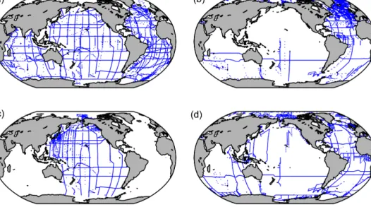
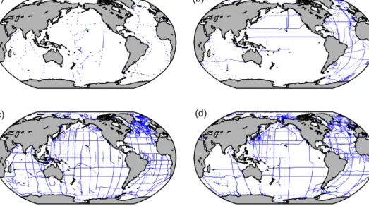
GLODAPv2 includes all data in GLODAPv1.1, CARINA, and PACIFICA, as well as data from 168 new cruises. The new data originate both from recent cruises, completed after production of the previous data syntheses, and from less re- cent cruises for which the data have only become available recently. Their sampling locations are shown alongside the
sampling locations of GLODAPv1.1, CARINA, and PACI- FICA cruises in Fig. 1. The new data were obtained by di- rectly contacting principal investigators known to have car- ried out relevant cruises and by circulating a request letter to the ocean carbon science community through the IOCCP, as well as the SOLAS and IMBER core projects of the IGBP. All of the new data are listed in the Supplement. For the cruises from GLODAPv1.1, CARINA, and PACIFICA the reader is referred to the web pages for each product at CDIAC.
Altogether, GLODAPv2 includes data from 724 cruises.
Data from the surveys of WOCE/JGOFS (King et al., 2001;
Sabine et al., 2005), CLIVAR, and GO-SHIP (Feely et al., 2014; Hood et al., 2010; Talley et al., 2016) form the back- bone. In addition, data from the large-scale surveys of the 1970s and 1980s – GEOSECS, TTO, and SAVE – and from a multitude of national and regional programs have been in- cluded. Examples include the time series stations KNOT, K2 (e.g., Wakita et al., 2010), and Line P (e.g., Wong et al., 2007) in the Pacific; the Indian Ocean INDIGO (e.g., Mantisi et al., 1991) and OISO (e.g., Metzl, 2009) programs; the Irminger and Iceland Sea time series data (Olafsson et al., 2009); and several Arctic Ocean (e.g., Jutterström and Anderson, 2005;
Giesbrecht et al., 2014) and Nordic Seas data (e.g., Jutter- ström et al., 2008; Olsen et al., 2010).
GLODAPv2 is primarily an open-ocean data product. Data from a few coastal surveys and time series have been in- cluded on an opportunistic basis. Time series data not in- cluded in GLODAPv2 include BATS (Steinberg et al., 2001) and HOT (Dore et al., 2003). The rationale is that the large amount of data from these time series would tend to bias the GLODAPv2 data product without improving its spatial de- tail, and the fact that these data are well maintained, orga- nized, and readily available.
3 GLODAPv2 methods 3.1 Primary quality control
All individual cruise data files used for GLODAPv1.1, CA- RINA, and PACIFICA existed in the required WOCE ex- change format and had been subjected to primary QC during the preparation of these products. All of the new data were merged as necessary, converted to WOCE exchange format, and also subjected to primary QC. The primary QC was car- ried out following routines outlined in Sabine et al. (2005) and Tanhua et al. (2010), primarily by inspecting property–
property plots. Outliers showing up in two or more different property–property plots were generally flagged as such. The WOCE QC flags are listed in Table 1. As with previous prod- ucts, a reduced flag set was used for the data product, while the full set was used for the individual cruise data files.
3.2 Secondary quality control
3.2.1 Merging of sensor and bottle data for salinity and oxygen
For salinity and oxygen, two types of submitted data exist.
Data files may have a single column of values for each, being either from analyses of water samples (in the following re- ferred to as bottle values/bottle salinity/bottle oxygen) or de- rived from CTD sensor pack data (in the following referred to as CTD values/CTD salinity/CTD oxygen). Otherwise, data files may include two columns of values, one containing the bottle values and the other the CTD values. For GLODAPv2 production the first type of data was subjected to crossover and inversion analysis (see Sect. 3.2.2) and bias-corrected whenever required, irrespective of them being bottle or CTD values.
For the data files including both CTD and bottle values, it was normally the CTD values that gave the complete profile, while the (likely more accurate) bottle values were sampled more sparsely. These data were therefore merged into single
“hybrid” salinity and oxygen prior to the crossover and inver- sion analyses. The consistency between CTD and bottle data from the same cruise was evaluated in this step. When sig- nificant offsets existed, the CTD data were corrected using a simple linear fit to the bottle data.
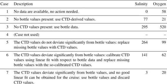
Altogether, seven possible scenarios were defined. The fourth never occurred, but it is included to maintain consis- tency with material produced during the secondary QC:
1. No data are available: no action needed.
2. No bottle values: use CTD values.
3. No CTD values: use bottle values.
4. Did not occur, case not used.
5. The CTD values do not deviate significantly from bottle values: replace missing bottle values with CTD values.
6. The CTD values deviate significantly from bottle val- ues: calibrate CTD values using linear fit with respect to bottle data and replace missing bottle values with the so-calibrated CTD values.
7. The CTD values deviate significantly from bottle val- ues, and no good linear fit can be obtained for the cruise:
use bottle values and discard CTD values.
The number of cases encountered for each scenario is sum- marized with the other secondary QC results for salinity and oxygen in Sects. 4.3.1 and 4.3.2. This merger step results in the GLODAPv2 data product having only a single column for salinity and a single column for oxygen. The original in- dividual cruise files contain salinity and oxygen (CTD and/or bottle) data as submitted by the data originator.
Figure 1.Station locations in(a)GLODAPv1.1,(b)CARINA, and(c)PACIFICA, as well as(d)locations of stations in GLODAPv2 new to data synthesis.
Table 1.WOCE flags in GLODAPv2 exchange format original data files and in product files (briefly for exchange files; for full details see http://geo.h2o.ucsd.edu/documentation/policies/Data_Evaluation_reference.pdf).
WOCE flag value Interpretation in original data/product files 0 Not used/interpolated or calculated value 1 Data not received/not useda
2 Acceptable/acceptable
3 Questionable/not usedb
4 Bad/not usedb
5 Value not reported/not useda 6 Average of replicate/not usedc
7 Manual chromatographic peak measurement/not usedc 8 Irregular digital peak measurement/not usedb
9 Sample not drawn/no data
aFlag set to 9 in product filesbData are not included in the GLODAPv2 product files and their flags are set to 9.cData are included but flag is set to 2.
3.2.2 Crossover and inversion analysis of salinity, oxygen, nutrients, TCO2, and TAlk
The secondary quality control of salinity, oxygen, nutrients, TCO2, and TAlk was carried out through crossover and in- version analyses. This two-step procedure was introduced by Gouretski and Jancke (2001) and Johnson et al. (2001). First, crossover analysis is used to determine cruise-by-cruise off- sets by comparing data where two different cruises cross or come close to each other. Next, possible corrections to data are determined in the inversion step. This uses least-squares models (Menke, 1984; Wunch, 1996) to calculate the set of corrections required to simultaneously minimize all cruise- by-cruise offsets. LetGbe the model matrix of sizeo×n, whereois number of crossovers andnnumber of cruises,d is theocrossover offsets, andmis thencorrections such that
G×m=d, (1)
then
m=GT ×(G×GT)−1×d. (2) This model is known as simple least squares (SLSQ).
Johnson et al. (2001) also introduced the weighted least squares (WLSQ) and weighted damped least squares (WDLSQ) models. The latter takes into account the uncer- tainties of the crossover offsets and a priori information on expected measurement accuracy of each cruise, while the for- mer only uses the uncertainties of the crossover offsets.
The crossover offsets can be determined in various ways.
For GLODAPv1.1 crossover offsets were calculated from stations within 1◦ (∼100 km) of each other. During CA- RINA, more elaborate and automated crossover methods
Table 2.Initial minimum adjustment limits introduced by CARINA and subsequently used for PACIFICA and GLODAPv2.
Variable Minimum adjustment Salinity 0.005
Oxygen 1 % Nutrients 2 % TCO2 4 µmol kg−1 TAlk 6 µmol kg−1
pH 0.005
CFCs 5 %
were developed, for example the “running-cluster” crossover routine, which determines the difference profiles for all sta- tion pairs within 200 km from each other. The crossover offset and its standard deviation are then calculated as the weighted mean and standard deviation of all difference pro- files. This is highly advantageous for comparing data from repeat sections (Tanhua et al., 2010).
The bias correction of the data included in GLODAPv2 is based on crossover and inversion analyses of the entire unad- justed database. The crossovers offsets were calculated using the running-cluster crossover routine (Tanhua et al., 2010), with data from beneath 2000 m to minimize effects of real variations. Only a fraction of the corrections determined by the crossover and inversion analyses were actually applied to adjust the data. For example, corrections lower than the expected measurement precision – or minimum adjustment limits (introduced by CARINA, Table 2) – were usually not applied, unless the data were very precise and evidence un- equivocal. Time trends in the data also give rise to correc- tions that should not be applied. All corrections were there- fore manually evaluated; those that were actually applied are called adjustments. While regional WLSQ inversions of the crossover offsets were used as a first step, they were usu- ally subsequently augmented with customized analyses to determine any underlying patterns and the final adjustments:
for example, invoking the assumption that cruises from the WOCE and CLIVAR surveys are of superior quality and may be used as core cruises in a WDLSQ inversion, or carrying out analyses on a subset of data from a given region. An over- all strategy was to use of a group of cruises with known high quality to form a cohesive grid against which cruises of un- known quality could be evaluated. Usually only one adjust- ment per cruise/leg was allowed for each variable – i.e., the underlying assumption for these analyses is that any bias is constant over the duration of the entire cruise/leg. In cases of obvious and significant drift or excessive scatter, all data for the variable at the cruise in question were usually excluded from the product.
In addition to the analyses of the entire and unadjusted dataset, several preliminary analyses were carried out. In particular, (1) GLODAPv1.1 was re-evaluated using the CARINA developed crossover and inversion tools, produc- ing GLODAPv1.2 (not publicly released), and (2) all new data were evaluated on an individual basis using crossovers against a preliminary global reference consisting of GLO- DAPv1.2 (i.e., re-evaluated GLODAPv1.1), CARINA, and PACIFICA combined, using a software package documented in Lauvset and Tanhua (2015). This is more extensively doc- umented in Appendix A. Familiarity with these preliminary analyses can be useful when accessing the documentation in the GLODAPv2 online Adjustment Table, which is described in Sect. 4.2.
For the Arctic Ocean, crossover and inversion analyses were used in combination with secondary QC procedures de- scribed by Jutterström et al. (2010), because of the sparse data and heterogeneous conditions. These include inspection of average property values in individual basins, and inspec- tion of deviations from the values derived using a set of mul- tiple linear regression (MLR) equations specific to the vari- ous regions.
3.2.3 Quality control of the halogenated transient tracer data
Given the strongly transient nature and low concentration of halogenated transient tracers (CFC-11, CFC-12, CFC-113, and CCl4; CFCs for short) in most deep waters, crossover and inversion analysis is of limited value for these variables.
Further, in the previous synthesis products the included CFCs had been subjected to quality control of varying extent:
– In GLODAPv1.1 they were subjected to full primary and secondary QC.
– In CARINA, the CFC data were subjected to full pri- mary and secondary QC in the Arctic and Atlantic re- gions, but not in the Southern Ocean region.
– No secondary QC was carried out for the PACIFICA CFC data.
Here, secondary QC of the CFC data focused on the 168 new cruises as well as the PACIFICA and Southern Ocean CA- RINA data. To ensure consistency, the GLODAPv1.1 CFC data were re-evaluated using the same procedures.
The CFC methods included inspection of surface satura- tion levels, evaluation of the relationships among the tracers from each cruise, and crossover and inversion analysis, all following CARINA protocols (Jeansson et al., 2010; Stein- feldt et al., 2010). Adjustments to CFC-113 and CCl4data have only been suggested in a few cases as their potential loss by decomposition in the water column renders secondary QC a questionable task. Secondary QC of sulfur hexafluoride (SF6) was not possible because few data were available.
3.2.4 Scale conversion and quality control of the pH data
In the three GLODAPv2 predecessors, pH data were treated in various ways:
– pH data were not included in the GLODAPv1.1 product files per se but were used in combination with TCO2to calculate TAlk whenever that was missing and pH avail- able. The TAlk data were then subjected to secondary QC.
– In CARINA, pH data were subjected to secondary QC and included in the regional product files (Velo et al., 2010). pH calculated from (quality-controlled) TCO2
and TAlk data were also included. The pH data included in the CARINA product files were unified to the seawa- ter scale (SWS) at 25◦C and surface (0 dbar) pressure.
– PACIFICA included measured as well as calculated pH data, like CARINA, but no secondary QC was pre- formed (Suzuki et al., 2013). The pH data were reported on the total hydrogen ion scale at 25◦C and surface (0 dbar) pressure.
For GLODAPv2 it was decided to include quality-controlled pH on the total hydrogen ion scale at both standard (25◦C and surface (0 dbar) pressure) and in situ (temperature and pressure) conditions. The total hydrogen ion scale was preferred, which has been recommended by Dickson et al. (2007) and by Dickson (2010).
Scale conversion of reported pH was carried out using the procedures of Velo et al. (2010), with the exception that, instead of the Merbach carbonate dissociation constants re- fitted by Dickson and Millero (Dickson and Millero, 1987;
Merbach et al., 1973), the ones of Lueker et al. (2000) were used. These are based on the measurements of Merbach et al. (1973) but made consistent with the total hydrogen ion scale. While the thermodynamic calculations themselves are easily performed with the CO2SYS toolbox (Lewis and Wal- lace, 1998; van Heuven et al., 2011) with the proper settings, missing or wrong information on scale and/or temperature and pressure conditions of reported data is not infrequent, which makes the scale conversion a challenging task. Hence, all reported pH data were compared with surrounding data for each cruise, as either observed or calculated from TCO2
and TAlk, in order to determine or verify the scale and con- ditions. This job was somewhat simplified as the pH scale of data from the CARINA and PACIFICA data syntheses has already been determined (Velo et al., 2010; Suzuki et al., 2013).
Crossover analysis of pH was not possible because data only exist for a small fraction of the cruises. Instead, one of three options was selected (in order of increasing complex- ity):
1. If pH was the only seawater CO2 chemistry variable measured at the cruise in question, or if the measure-
ments had not been carried out at the same stations and/or depths as the other CO2chemistry data, the pH values were inspected for spread. If this appeared ac- ceptable, then the data were kept but were labeled as not subjected to full secondary QC (−888; see Sect. 4.2).
2. If the pH data were accompanied by (unbiased or bias- corrected) TCO2andTAlk data, the internal consistency of the measurements was evaluated and used to adjust (or in some cases discard) the pH data if these appeared offset.
3. If the pH data were accompanied by (unbiased or bias-corrected) TCO2orTalk (allowing calculations of TAlkorTCO2) and collocated with (unbiased or bias- corrected) measured data of TAlk or TCO2 of other cruises, crossover analysis was preformed between cal- culated and measured data of respective cruises. If the calculated TAlk (or TCO2) values were offset from the measured values of the other cruise, the pH data of the cruise of interest were adjusted to minimize this offset (provided that the scatter in the pH data was acceptable;
otherwise, they were discarded).
The NBS scale for pH measurements has large inherent un- certainties (Dickson, 1984). Recognizing this, such data have not been included in the data product unless passing full sec- ondary QC, criteria 2 or 3.
4 GLODAPv2 secondary QC results and adjustments
4.1 Preservation of real variability
The risk of removing real signals of variability present in the data was recognized throughout secondary quality control, in particular because the crossover and inversion is an objec- tive method that does not discriminate between real differ- ence and measurement bias. By only using data deeper than 2000 m for crossover analyses, this risk was reduced, but in some regions deep-water time trends are expected to occur over the decadal timescales considered. Therefore, each cor- rection suggested by the crossover and inversion analysis was scrutinized. Whenever doubt existed, adjustments were not applied, in particular in regions of strong variability (such as the Nordic Seas overflow), or when time trends were de- tected or suspected. As an example of a method of preserv- ing trends, Fig. 2 shows one type of figure used to evaluate the crossover offsets. This particular cruise (18HU19960512) is an occupation of WOCE line AR07W in the Labrador Sea, and the crossover offsets indicate a bias in TCO2 of
−6 µmol kg−1, and the inversion suggested a correction of the same magnitude. However, plotting the crossover off- sets vs. time as in Fig. 2 clearly reveals the strong TCO2 trend. The gradual decrease in the offsets implies a tempo- ral TCO2 increase at depth rather than a negative bias (as
implied by the mean of the offsets). This is consistent with anthropogenic CO2uptake and the deep mixing that occurs in this region (Yashayaev, 2007). Cruise 18HU19960512 is not appreciably offset from contemporaneous cruises. No adjust- ments were applied to these data.
4.2 The adjustment table
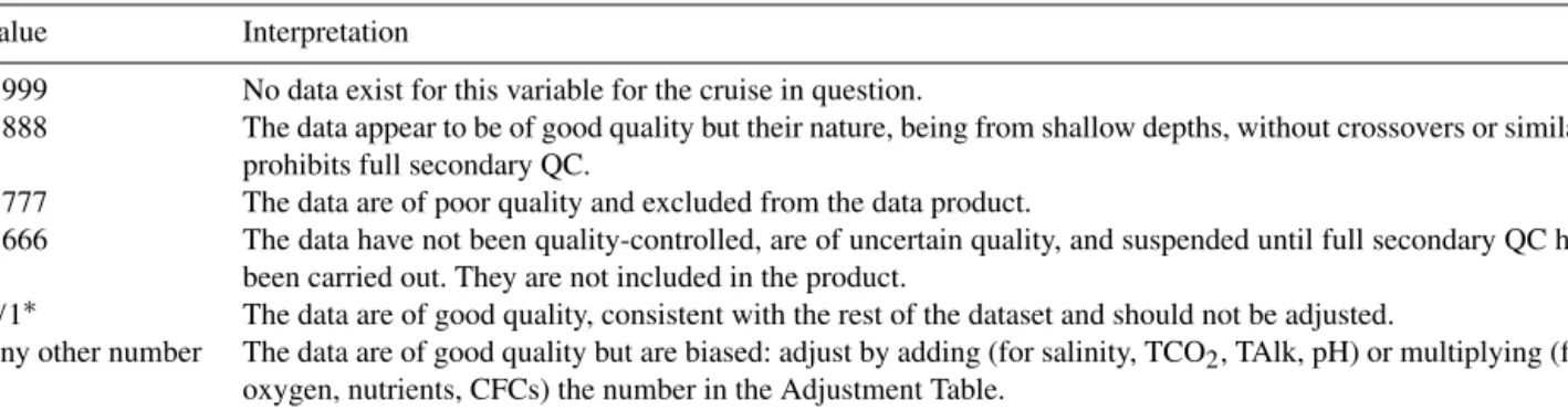
The results of the secondary QC analyses were entered into the online GLODAPv2 Adjustment Table hosted at GEO- MAR in Kiel, Germany. This is similar in form and func- tion to the Adjustment Table used in CARINA (Tanhua et al., 2010). A permanent, non-editable version of this Adjustment Table is available at http://glodapv2.geomar.de. Table 3 sum- marizes the type of entries in the Adjustment Table. In con- trast to CARINA, the GLODAPv2 Adjustment Table does not include an entry for each crossover; the large number of crossover locations made this unmanageable. Even though at many locations either of the involved cruises may not have the required deep, high-quality data, the number of success- fully assessed crossovers ranges from ∼3400 for TAlk to
∼12 100 for salinity. Hence, there is one entry per cruise, providing access to summary figures from the crossover anal- ysis and the magnitude and justification of any recommended adjustments. Further details are provided in Appendix B.
4.3 Secondary QC summary
Data from 734 cruises were subjected to secondary QC. For 10 of these the secondary QC revealed that most if not all of the data were of unacceptable quality. Further, for these 10 cruises, better quality data from the same region were avail- able, and they were therefore not included in the final prod- uct files. The original data from these 10 cruises are avail- able through the Cruise Summary Table (CST, see Sect. 5.1) at CDIAC, at the very end of the CST. They have been as- signed cruise number 9999 and secondary QC results are not included in the summaries below.
GLODAPv2 thus includes data from 724 cruises. These were split into a total of 780 cruises/legs/station ranges dur- ing secondary QC. This is partly because most cruises con- sisting of individual legs were analyzed on a per-leg basis (Table 4) in order to take into account potential changes in personnel, equipment, and procedures during their execution and partly because four cruises were adjusted on a per-station range basis as a result of obvious bias in one or several vari- ables for specific parts of, but not the entire, cruise (these are 74AB20050501, 316N19831007, 06GA20000506, and 06AQ19920521). Respecting this distinction, we therefore refer in the following summary to analyzed “entries” instead of cruises, where an entry is an entire cruise (the large ma- jority), leg, or station range.
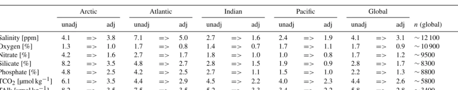
Application of adjustments was done with the aim of re- ducing the deep-water offsets between the many entries. A measure of this reduction is given by the “internal consis-
tency improvement”. This is the decrease in the weighted mean of the absolute offsets of all crossovers between (i) the unadjusted data (after primary QC) and (ii) the adjusted data (after secondary QC) (Tanhua et al., 2010). This is not the only means of quantifying improvement, but it is a good compromise in terms of implementation, clarity, and brevity. Certainly, improvement will be different between ge- ographical regions, vessels, labs, and countries, with small- est improvements generally observed between the large hy- drographic repeat surveys. Conversely, appreciable local im- provements are observed for smaller cruises run by groups without a primary focus of delivering climate-quality data (e.g., biological process studies). While the interesting na- ture of these details is recognized, Table 5 only provides the improvements per ocean basin and for the full world ocean.
The relative improvement for nutrients, TCO2, and TAlk is higher than for salinity. Salinity accuracy was quite high for most cruises already. The internal consistency of all variables subjected to secondary QC has been increased significantly.
Summaries of the secondary QC actions are presented in Tables 6 and 7. Figure 3 summarizes the distribution of the adjustments that were applied. Details on the secondary QC results are presented per variable in the following subsec- tions.
4.3.1 Salinity merging and adjustment summary
All 780 entries came with salinity data (Table 6). Prior to the crossover and inversion analyses, the CTD and bottle salinity values were merged as described in Sect. 3.2.1. The different actions in this respect are summarized in Table 8.
After the data were merged, they were subjected to crossover and inversion analyses. For 162 of the entries, full secondary QC could not be carried out, and data from 6 en- tries were deemed to be of too poor a quality for inclusion in GLODAPv2 (Table 6). Typically, these showed large and depth-dependent offsets and/or unrealistic scatter compared to background data. Of the remaining 612 entries, the salin- ity data from 41 were found clearly biased, warranting an adjustment (Table 6).
Adjustments smaller than the initial threshold have only been applied to five entries, while the bulk of the ad- justments applied are between 0.005 and 0.010 (Table 7, Fig. 3g). The largest negative and positive adjustments ap- plied are−0.025 and+0.025. Application of the adjustments increased the global consistency of the salinity data from 0.0041 to 0.0031 as evaluated from the weighted mean of the absolute crossover offsets (Table 5).
4.3.2 Oxygen merging and adjustment summary Of the 780 entries, 722 had oxygen data (Table 6). Data of CTD and chemically determined oxygen concentration were merged into a single, “hybrid” variable using procedures in Sect. 3.2.1, with results summarized in Table 8. Crossover,
1970 1975 1980 1985 1990 1995 2000 2005 2010 2015
−15
−10
−5 0 5
Mean±se of offsets: -6.1 0.7 SD of offsets: 3.6, n=25
316N19810401.6 18HU19920527 18HU19930617 18HU19940524 18HU19950607 18HU19970509 06MT19970707 18HU19980622 06MT19990711 18HU19990627 18HU20000520 06MT20010507 18HU20010530 18HU20020623 18HU20030713 06MT20030723 18HU20040515 18HU20050526 18HU20060524 18HU20070510 18HU20080520 74DI20080820 18HU20090517 18HU20100513 18HU20110506
Year
TCO2 offsets between 18HU19960512 and other cruises
Offset [µmol kg]-1
±
Figure 2.Summary figure used to evaluate TCO2crossover offsets of WOCE repeat section AR07W cruise 18HU19960512 in the Labrador Sea. The figure shows the 25 crossover offsets that were determined, sorted by time. 18HU19960512 is indicated by the blue line. Negative values mean that 18HU19960512 TCO2values are lower than those of the comparison cruise.
Table 3.Possible values in the Adjustment Table and their interpretation.
Value Interpretation
−999 No data exist for this variable for the cruise in question.
−888 The data appear to be of good quality but their nature, being from shallow depths, without crossovers or similar, prohibits full secondary QC.
−777 The data are of poor quality and excluded from the data product.
−666 The data have not been quality-controlled, are of uncertain quality, and suspended until full secondary QC has been carried out. They are not included in the product.
0/1∗ The data are of good quality, consistent with the rest of the dataset and should not be adjusted.
Any other number The data are of good quality but are biased: adjust by adding (for salinity, TCO2, TAlk, pH) or multiplying (for oxygen, nutrients, CFCs) the number in the Adjustment Table.
∗The value of 0 is used for variables with additive adjustments (salinity, TCO2, TAlk, pH) and 1 for variables with multiplicative adjustments (for oxygen, nutrients, CFCs).
This is mathematically equivalent to “no adjustment” in each case.
inversion, and subsequent adjustment for bias minimization were performed on this hybrid oxygen. A total of 378 of the entries were deemed to be accurate to within the minimum adjustment limits, and thus did not require an adjustment (Ta- ble 6). A total of seven applied non-zero adjustments were smaller than the threshold of 1 % (Table 7, Fig. 3f). These necessarily were cruises with sufficiently high precision so that such small bias could be observed beyond doubt. Al- most half of the non-zero adjustments were between 1 and 2 %, while the other half of the applied non-zero adjust- ments (99 cruises) was greater than 2 % (Table 7, Fig. 3f).
The largest adjustments applied were−7.2 and+11 %. This rather tight distribution is testimony to the high accuracy gen- erally achieved in oxygen measurements.
4.3.3 Nitrate adjustment summary
Nitrate data were available for 709 of the 780 entries (Ta- ble 6). Of these, data from 42 were of insufficient qual- ity for inclusion, data from 137 could not be fully quality- controlled, and data from 530 received successful secondary QC (Table 6). Of these, 380 were accepted to be accurate and 150 entries were adjusted. Of the applied adjustments, 50 (i.e., 33 %) are beneath the initial 2 % limit, while 49 % are between 2 and 4 % (Table 7, Fig. 3b). The high frac- tion receiving small adjustments illustrates the high preci- sion commonly attained with nitrate analysis. The secondary nitrate QC was performed without notable peculiarities. Sec- ondary QC markedly increased the internal consistency of the nitrate data (Table 5). This suggests (i) that the nitrate data are generally highly precise (while not necessarily ac- curate), and (ii) that our assumption that each entry suffered from not more than one, constant bias is generally valid. Very
Table 4.Multi-leg cruises in GLODAPv2 that received secondary quality control on a per-leg basis but are included as a single cruise in the product files.
Cruise number EXPOCODE Expocodes of individual legs
102 18DD19940906 18DD19940906; 18DD19941013
236 316N19720718 316N19720718.1; 316N19720718.2; 316N19720718.3;
316N19720718.4; 316N19720718.5; 316N19720718.6;
316N19720718.7; 316N19720718.8; 316N19720718.9 237 316N19810401 316N19810401; 316N19810416; 316N19810516;
316N19810619; 316N19810721; 316N19810821;
316N19810923
238 316N19821201 316N19821201; 316N19821229; 316N19830130 242 316N19871123 316N19871123.1; 316N19871123.2; 316N19871123.3;
316N19871123.4; 316N19871123.5; 316N19871123.6 243 316N19920502 316N19920502; 316N19920530; 316N19920713 255 316N19950829 316N19950829; 316N19950930
257 316N19951202 316N19951202; 316N19951230
268 318M19730822 318M19730822; 318M19730915; 318M19731007;
318M19731031; 318M19731204; 318M19740102;
318M19740205; 318M19740313; 318M19740412;
318M19740513
269 318M19771204 318M19771204; 318M19771216; 318M19780128;
318M19780307; 318M19780404
273 318M20091121 318M20091121; 318M20100105
298 325019850330 325019850330; 325019850504
319 32MW19890206 32MW19890206; 32MW19890309; 32MW19890402
338 33MW19930704 33MW19930704.1; 33MW19930704.2
370 35MF19850224 35MF19850224; 35MF19860401; 35MF19870114
439 49HH19910813 49HH19910813; 49HH19910917
486 49NZ20030803 49NZ20030803; 49NZ20030909
497 49NZ20051031 49NZ20051031; 49NZ20051127
507 49NZ20090410 49NZ20090410; 49NZ20090521
Table 5.Improvements resulting from the GLODAPv2 quality control split out per basin and for the global dataset. The numbers in the table are the weighted mean of the absolute offsets of all crossovers of unadjusted and adjusted data, respectively.nis the total number of valid crossovers in the global ocean for the variable in question.
Arctic Atlantic Indian Pacific Global
unadj adj unadj adj unadj adj unadj adj unadj adj n(global)
Salinity [ppm] 4.1 => 3.8 7.1 => 5.0 2.7 => 1.6 2.4 => 1.9 4.1 => 3.1 ∼12 100
Oxygen [%] 1.3 => 1.0 1.7 => 0.8 1.4 => 0.7 1.7 => 1.1 1.7 => 0.9 ∼10 900
Nitrate [%] 4.2 => 1.6 2.7 => 1.7 1.8 => 1.0 1.0 => 0.8 1.7 => 1.2 ∼9500
Silicate [%] 8.2 => 3.5 4.8 => 2.7 2.8 => 1.5 1.9 => 0.9 2.8 => 1.7 ∼8300
Phosphate [%] 4.8 => 2.5 4.2 => 2.5 2.7 => 1.1 1.5 => 1.0 2.2 => 1.3 ∼8800
TCO2[µmol kg−1] 6.1 => 3.5 4.4 => 2.9 4.5 => 2.2 4.0 => 2.3 4.4 => 2.6 ∼5800 TAlk [µmol kg−1] 8.2 => 3.5 7.5 => 3.5 5.2 => 3.3 3.4 => 2.2 5.8 => 2.8 ∼3400
few exceptions were encountered that exhibited either strong instrumental drift or strong station-to-station variability.
The southeastern corner of the Pacific (30–90◦S, 120–
70◦W) is a region of particular uncertainty for nitrate. The data do not form a cohesive network with an unambiguous
“baseline”. An important source of uncertainty here is drift of the nitrate measurements from 33RO20071215 and/or 31DS19940124.
4.3.4 Silicate adjustment summary
Silicate data were available for 678 of the 780 entries (Ta- ble 6). The silicate data of 33 entries were found to be of poor quality, exhibiting excessive scatter, large offsets, drift, or a combination of these. For 255 entries the silicate data were considered to be accurate to within the uncertainty of our methods, while data from 264 entries were adjusted (Ta- ble 6). This is almost 40 % of the entries, making silicate the
0 10 20 30 40 TCO2
Adj. mean: -2.5 Adj. sd.: 13.9
(a)
No.
0 20 40 60 80 TAlk
Adj. mean: -3.4 Adj. sd.: 12.2
(d)
No.
0 5 10 AA
Salinity (*1000) Adj. mean: 1.0 Adj. sd.: 11.2
(g)
No.
−40 −20 0 20 40
0 2 4 6 A 8 pH (*1000)
Adj. mean: -5.0 Adj. sd.: 22.5
(j)
No.
Adjustment
Nitrate Adj. mean: -0.0 % Adj. sd.: 3.5 %
(b)
Silicate Adj. mean: 0.2 % Adj. sd.: 3.5 %
(e)
CFC−11 Adj. mean: 1.3 % Adj. sd.: 8.8 %
(h)
−15 −10 −5 0 5 10 15 CFC−113
Adj. mean: 3.3 % Adj. sd.: 8.8 %
(k)
Adjustment (%)
Phosphate Adj. mean: 0.5 % Adj. sd.: 3.9 %
(c)
Oxygen Adj. mean: -0.4 % Adj. sd.: 2.9 %
(f)
CFC−12 Adj. mean: -1.9 % Adj. sd.: 8.0 %
(i)
−15 −10 −5 0 5 10 15 CCl4
Adj. mean: -2.0 % Adj. sd.: 9.1 %
(l)
Adjustment (%)
Figure 3.Size distribution of applied adjustments for each core variable that received secondary QC. Gray areas depict the initial minimum adjustment limit. Entries for which data could not be secondary quality-controlled or were considered of insufficient quality for our product are excluded from this figure.
Table 6.Summary of secondary QC actions per variable for the 780 non-dismissed entries.
Salinity Oxygen Nitrate Silicate Phosphate TCO2 TAlk pH CFC-11 CFC-12 CFC-113 CCl4
With data 780 722 709 678 688 602 465 259 273 270 105 72
No data 0 58 71 102 92 178 315 521 507 510 675 708
Unadjusteda 571 378 380 255 282 332 180 59 208 207 57 33
Adjustedb 41 207 150 264 163 104 150 77 26 19 6 5
−888c 162 127 137 126 184 151 106 67 30 30 15 14
−666d 0 0 0 0 0 0 0 47 0 0 0 0
−777e 6 10 42 33 59 15 29 9 9 14 27 20
aThe data are included in the data product file as is, with a secondary QC flag of 1 (Sect. 5.2).bThe adjusted data are included in the data product file with a secondary QC flag of 1 (Sect. 5.2).cData appear of good quality but have not been subjected to full secondary QC. They are included in data product with a secondary QC flag of 0 (Sect. 5.2).dData are of uncertain quality and suspended until full secondary QC has been carried out; they are excluded from the data product.eData are of poor quality and excluded from the data product.
most frequently adjusted variable in GLODAPv2. The sin- gle reason for this is that the silicate data of a large fraction of Pacific entries were adjusted to remove an average 2 % offset in silicate observed between the US and Japanese en- tries from this region. This systematic “country-specific” bias was revealed by the crossover and inversion analyses. Fig- ure 4a and b present silicate biases between US and Japanese – uncorrected – cruises in the Pacific, from a dedicated inver- sion analysis of these data. It is evident from these that US silicate data tend to be approximately 2 % higher than the Japanese values. This systematic bias has been hinted at by results from laboratory comparison exercises (Aoyama et al.,
2010; S. Becker, Scripps, personal communication, 2014; K.
Bakker, NIOZ, personal communication, 2014). Kanso ref- erence material for nutrients in seawater (RMNS) samples were analyzed on several of the cruises involved, but the re- sults were not consistently used for correction since the as- signed values had not yet been certified (S. Becker, personal communication, 2014). While it would appear reasonable to assume that one country’s data should receive a 2 % cor- rection, the data and evidence are inadequate to determine which. The biases determined by the inversion provide no information in this respect: the lower mean bias of Japanese cruises is just a consequence of the zero-sum constraint of
Table 7.Summary of the distribution of applied adjustments per variable, in number of adjustments applied for each variable.
adj.<limit limit≤adj.<2×limit 2×limit≤adj.
Salinity 5 22 14
Oxygen 7 101 99
Nitrate 50 73 27
Silicate 113 95 56
Phosphate 31 92 40
TCO2 8 51 45
TAlk 37 76 37
pH 0 25 52
CFC-11 0 17 9
CFC-12 0 12 7
CFC-113 0 2 4
CCl4 0 2 3
Table 8.Summary of salinity and oxygen merger actions for the 780 non-dismissed entries subjected to secondary QC.
Case Description Salinity Oxygen
1 No data are available, no action needed. 0 58
2 No bottle values present: use CTD-derived values. 77 21
3 No CTD values present: use bottle data. 295 520
4 (Case not used) – –
5 The CTD values do not deviate significantly from bottle values: replace missing bottle values with CTD values.
264 99
6 The CTD values deviate significantly from bottle values: calibrate CTD values using linear fit with respect to bottle data and replace missing bottle values with the so-calibrated CTD values.
141 62
7 The CTD values deviate significantly from bottle values, and no good linear fit can be obtained for the cruise: use bottle values and discard CTD values.
3 20
the inversion combined with the larger number of Japanese cruises. The sum of all corrections suggested by the inver- sion has to be zero and the crossover and inversion tends to conclude that the most frequently measured value is the least biased one. In this case it is the deep silicate measured at Japanese cruises, since there are more Japanese than US cruises; hence, these come out with smaller mean bias than the US cruises, while the “true” value is unknown. Thus, to remedy this inconsistency the Japanese data were pre- adjusted by+1 % and US data by−1 %. This removed the systematic difference and a clear baseline emerged (Fig. 4c and d).
After this pre-adjustment, the set of Pacific silicate data were subjected to regular crossover and inversion analysis to obtain the total required correction. Note that the choice of splitting the difference between the US and Japanese ef- forts may result in the Pacific Ocean data product being – at least – between −1 and+1 % biased against the “true”
level. However, for the purposes of this data product such
residual, systemic, bias between the Pacific and the other major ocean basins (Atlantic, Arctic, Indian) is currently not seen as problematic. Nonetheless, reconciliation between the Japanese and US results should be a high priority for the nu- trient analytical community.
For the South Atlantic and Indian basins, crossover and inversion were performed without notable incidents.
Bias minimization of silicate was rather challenging in the North Atlantic Ocean, where silicate values may range from near zero at the ocean surface to well over 50 µmol kg−1 at depth. At the low end of that range, additive calibration biases manifest themselves in addition to the multiplicative ones the methods were designed to deal with (e.g., resid- ual silicate in the “nutrient-free” seawater used for standards preparation). Additionally, samples with nominal silicate val- ues over∼50 µmol kg−1 tend to be very sensitive to freez- ing, which can decrease the measured concentration by up to 15 % due to polymerization (Karel Bakker, NIOZ, personal communication, 2014). Samples with lower silicate concen-
1980 1985 1990 1995 2000 2005 2010
−8
−6
−4
−2 0 2 4 6 8
Year of cruise
Inferred bias [%]
Japan mean bias: −0.1 US mean bias: +0.4
−8
−6
−4
−2 0 2 4 6 8
Inferred bias [%]
Japan mean bias: −0.6 US mean bias: +1.7
Japanese datasets US datasets
(a) (b)
(c) (d)
Figure 4.Silicate biases between US and Japanese efforts before (a, b)and after(c, d)pre-adjustments (US:−1 %; Japan:+1 %) were applied to the data (see main text for details). Data from “Line P” and many small-scale cruises in the variable Kuroshio region were excluded from this analysis. Red and blue horizontal lines in- dicate countries’ approximate mean offsets.
tration seem to not be affected by freezing. Freezing was oc- casionally suspected (and then generally confirmed) to have been used on cruises, forcing arbitrary removal of data, and complicating the automated crossover analysis. Although the average offset for silicate at crossovers has been reduced in the North Atlantic Ocean, the solution there is not particu- larly satisfying and a more thorough assessment is expected to be able to substantially improve our results locally.
Overall, the application of the adjustments improved the global consistency of the silicate data by more than a percent, but with regional differences. In the Arctic the secondary QC has been in particular effective; consistency has been im- proved from 8.2 to 3.5 % (Table 5). This may also be due to removal of obviously poor data from some cruises in this region (see Fig. 7 for regional distributions of data).
4.3.5 Phosphate adjustment summary
A total of 688 entries included phosphate data (Table 6). Of these, data from 59 were found to be of too poor a quality for inclusion in the product. Adjustments were applied to 163 en- tries. Data from 184 entries could not be adequately checked with our routines.
Of the 163 adjusted entries, 31 (highly precise) received adjustments smaller than the threshold; 132 entries had larger adjustments (Table 7, Fig. 3c), with the largest being about
±12 %.
4.3.6 TCO2adjustment summary
TCO2was measured on 602 of the 780 entries (Table 6). The quality of 15 were too poor to be retained. Data from 151 were not fully quality-controlled, and of the remainder, 332 entries were accurate within the uncertainty of our methods and 104 were adjusted. The minimum TCO2adjustment was initially set to 4 µmol kg−1. For eight very precise entries a smaller adjustment was applied (Table 7, Fig. 3a). A few very large adjustments were applied, generally to historic entries (e.g., GEOSECS).
Globally the consistency has improved by 1.8 µmol kg−1, and by much more in some regions (Table 5). The largest improvement is observed for data from the Arctic region.
4.3.7 TAlk adjustment summary
In total, 465 entries had TAlk data; 106 of these could not be subjected to full secondary QC and were set to −888 (Table 6). Of the remainder, 29 were deemed too poor for inclusion, 180 were of good quality and unbiased, and 150 needed adjustment. The initial minimum allowable adjust- ment was 6 µmol kg−1(Table 2). About 75 % of the applied adjustments are equal to or larger than this (Table 7, Fig. 3d).
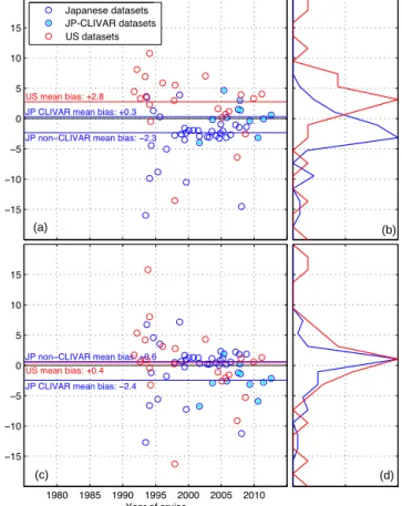
TAlk is the second most frequently adjusted variable in GLO- DAPv2 with 32 % recommended for adjustment. This was the result of a bias identified in Japanese Pacific cruises. Fol- lowing crossover and inversion analysis a very clear separa- tion was observed between the US entries and (most of) the Japanese Pacific entries. This is illustrated in Fig. 5a and b.
Japanese data appear consistently too low, while US data ap- pear consistently high. The offset between US and Japanese labs appears to exist throughout the era of measurements, al- though too few data exist in the latest 10 years to be sure.
Typically, the available metadata for the Japanese cruises were sparse and did not include information on traceability to CRMs. However, the six or so Japanese results after 2005 that were found tonotrequire an adjustment relative to the US were all CLIVAR/GO-SHIP lines. A possible explana- tion is that these Japanese CLIVAR/GO-SHIP measurements have been standardized against the certified reference mate- rial provided by A. G. Dickson (Dickson, 2001; Dickson et al., 2003), whereas the smaller Japanese lines have used a
1980 1985 1990 1995 2000 2005 2010
−15
−10
−5 0 5 10 15
Year of cruise Inferred bias [µmol kg-1]
JP CLIVAR mean bias: −2.4 JP non−CLIVAR mean bias: +0.6 US mean bias: +0.4
−15
−10
−5 0 5 10 15
Inferred bias [µmol kg-1]
JP CLIVAR mean bias: +0.3 JP non−CLIVAR mean bias: −2.3 US mean bias: +2.8
Japanese datasets JP-CLIVAR datasets US datasets
(a) (b)
(c) (d)
Figure 5. TAlk biases between US and Japanese efforts before (a, b) and after(c, d)pre-adjustments were applied to TAlk data of Japanese non-CLIVAR cruises (see main text for details). Cir- cles represent the biases (inferred by the GLODAPv2 inversion method) of TAlk measurements of individual cruises in the Pacific Ocean. Data of “Line P” and many small-scale cruises in the vari- able Kuroshio region were excluded from this analysis. Red and blue horizontal lines indicate countries’ approximate mean offset.
For Japanese data the values are split into cruises that were or were not part of CLIVAR.
different method of standardization. Some additional infor- mation may be gleaned from assessing these results on a per- ship or per-lab basis rather than per-country, but such analy- ses have not been performed. As has been noted earlier, the crossover and inversion method does not provide any infor- mation about which set of data is the correct one. For silicate the difference was split between Japanese and US cruises, in the absence of additional information. In this case, based on thedocumentedtraceability to CRM for the US cruises, a +6 µmol kg−1pre-adjustment was applied to the TAlk of the Japanese non-CLIVAR Pacific cruises. This is the reason for the peak in the distribution of applied adjustments visualized in Fig. 3d. The consistency of US and Japanese Pacific TAlk data after the pre-adjustment is shown in Fig. 5c and d. Note that the average corrections are now essentially identical for both countries and close to zero.
After this pre-adjustment, the set of Pacific TAlk data were subjected to regular crossover and inversion analysis to ob- tain the total required correction.
4.3.8 pH adjustment summary
A total of 259 entries included pH data (Table 6). Of these, 59 were found accurate, while 77 were adjusted; 67 could not be fully quality-controlled but are thought to be accurate (−888). Data from 47 cruises were suspended and further QC is required. These are all data supplied on the NBS scale (Sect. 3.2.4).
4.3.9 CFC-11, CFC-12, CFC-113, and CCl4adjustment summary
During WOCE and CLIVAR, CFC-11 and CFC-12 were commonly measured, whereas data for CFC-113 and CCl4 are less abundant. This is reflected in the number of entries with CFC data available in GLODAPv2 (Table 6: 273/270 for CFC-11/CFC-12, but only 105 for CFC-113 and 72 for CCl4). The range of CFC concentrations in deep water spans about 2 orders of magnitude (∼0.01 to 1.0 pmol kg−1). Areas with higher concentration are often subject to temporal vari- ability, as they are close to the deep-water formation areas.
In regions with less temporal variability, CFC concentrations are low, and a relative error of∼10 % might still be smaller than the accuracy of the data. Consequently, data adjustment is more difficult than for other variables. The threshold for adjustment was set to 5 % as in CARINA. As a result, only about 10 % of the CFC data have been corrected, less than for the other quantities (Table 6). Quality control of CFC-113 and CCl4is even more difficult. For these two, adjustments have only been applied if repeat cruises from the same area were available and the data from these repeats were clearly inconsistent. For applied CFC-113 and CCl4 adjustments, about 65 % are larger than 10 %, or 2 times the limit. Only about 35 % of adjustments for CFC-11 and CFC-12 are that large (Table 7 and Fig. 3h, i, k, l).
5 GLODAPv2 product access and description GLODAPv2 consists of three components: the original data, the bias-corrected product files, and the mapped climatology.
They are available at CDIAC (http://cdiac.ornl.gov/oceans/
GLODAPv2/). The original data and product files are de- scribed here, while the mapped climatology is described by Lauvset et al. (2016).
5.1 Original data
GLODAPv2 includes original data from 724 cruises, and ac- cess and documentation for individual cruise files are pro- vided through the CST at the GLODAPv2 web page at CDIAC. The 724 cruises may consist of several legs, and
in a few cases multiple cruises have been merged. Among other things, the CST includes a column that lists individual components of multi-leg cruises analyzed per leg (Sect. 4.3).
The content of the original data files is as received from the originator, but the files have been updated to WOCE ex- change format (Swift and Diggs, 2008) whenever required.
File headers, listing essential information on cruises and the analytical procedures, were generated for all except the PACIFICA cruises. No bias adjustments were applied to the data in these files, and they also contain the oxygen and salin- ity data as submitted – i.e., no merged bottle and CTD values are included.
Each cruise and data file is uniquely identified with its GLODAPv2 cruise number and its EXPOCODE. Known aliases are also specified in the CST. The GLODAPv2 cruise numbers were assigned sequentially after sorting by EXPOCODE. EXPOCODES were constructed by com- bining the NODC platform code (http://www.nodc.noaa.
gov/General/NODC-Archive/platformlist.txt) with the sail- ing date of the cruise in the format YYYYMMDD. In a few cases when the sailing date could not be determined, the date of the first sampling was used. After the inception of GLO- DAPv2, the responsibility for platform code assignment was assumed by the ICES data center (http://ices.dk/marine-data/
vocabularies/Pages/default.aspx). A few differences exist be- tween the two sets of codes; the older or better-known code was preferred in these cases.
Note that, for the following time series or campaigns, the data have not been segmented into individual cruises but in- stead maintained as collections under a single EXPOCODE, to ease record keeping: the EGEE, GIFT, Iceland Sea, Irminger Sea, Kerfix, OWS Mike, and SWITCHYARD time series (assigned EXPOCODES are 35A820050607, CAR- BOGIB2005, IcelandSea, IrmingerSea, 35UCKERFIXTS, 58P320011031, and ZZIC2005SWYD), and the OMEX- 1 Nordic Seas, OMEX-1 North Atlantic, and OMEX- 2 North Atlantic campaigns (assigned EXPOCODES are OMEX1NS, OMEX1NA, and OMEX2NA).
All concentration units are those set for WOCE and used in earlier data products. In particular, any oxygen and nutrient concentrations reported in milliliters or micromoles per liter were converted to micromoles per kilogram (µmol kg−1).
The default procedure for nutrients was to use seawater den- sity at reported salinity, an assumed lab temperature of 22◦C, and a pressure of 1 atm. The error made by an actual lab temperature deviating up to 5◦C from the assumed 22◦C is insignificant. For the milliliter to micromole conversion for oxygen, the factor 44.66 was used, derived using the ideal gas law at standard temperature and pressure, corrected for the non-ideal behavior of oxygen, while for the per-liter to per-kilogram conversion potential density was used when- ever draw temperatures were unavailable.
Note also that the original TTO-NAS data file contains the potentiometrically measured TCO2 and non-adjusted TAlk, while the data product contains the adjusted and calculated
TAlk and TCO2derived using the recommendations by Tan- hua and Wallace (2005).
WOCE quality flags (Table 1) have been applied through- out. Any questionable or bad data identified during primary QC are included and flagged accordingly in these files. How- ever, note that whenever data from an entire cruise were found to be bad following secondary QC, they have not nec- essarily been flagged as such in the individual data files.
However, this may be noted in the metadata, and is definitely noted in the Adjustment Table at GEOMAR. The Adjustment Table record for each specific cruise can be directly accessed via the hyperlink that appears in the rightmost column in the CST. All users of the individual cruise data files are en- couraged to respect the WOCE flags that have been applied and also to consult the notes in the Adjustment Table and all available metadata before any analyses are carried out. Meta- data for each cruise is usually contained in the header of each exchange file and/or in the “Metadata” link in the CST. These two sources can be complementary. For many cruises, access to copies of written cruise reports is provided through the CST, as well as references to relevant scientific publications.
5.2 Product files
The GLODAPv2 data product is available as one global file containing all 724 cruises, with bias minimization adjust- ments applied to the data. Cruises are in alphabetical order of EXPOCODES. In addition, four regional subset files have been produced: one each for the Arctic, Atlantic, Pacific, and Indian oceans. The global decadal coverage of GLO- DAPv2 is given in Fig. 6, and that of each regional file in Fig. 7. The files are available as comma-separated ASCII files (*.csv) and as binary MATLAB format files (*.mat;
MATLAB, 2015).
There is no data overlap in the regional files – i.e., a single cruise can only appear in one of the regional files even though some cruises cover multiple basins. In the product files each cruise is identified using its unique GLODAPv2 cruise num- ber to avoid text strings in the data files, i.e., EXPOCODES are not included. In the global file, cruise numbers increase consecutively, while cruise numbers in the regional subset files increase but are not consecutive. A lookup table is pro- vided with the data files to facilitate matching of cruise num- ber and EXPOCODE. In the MATLAB version of the prod- uct files, a structure array named “expocodes” is available, containing all 724 EXPOCODES.
The product files were prepared following the same gen- eral procedures used for GLODAPv1.1 (Key et al., 2004;
Sabine et al., 2005) and CARINA (Key et al., 2010) and are only summarized here:
1. If temperature was missing, then all data for that record were set to−9999/NaN and their flags to 9. The same was done when pressure/depth was missing, except for the 911 records that were associated with Niskin bottle
Figure 6.Station locations in the GLODAPv2 data product for data obtained during(a)the 1970s,(b)the 1980s,(c)the 1990s, and(d)2000s and beyond.
Figure 7.Locations of data included in the(a)Arctic,(b)Atlantic,(c)Indian, and(d)Pacific ocean product files. Note the minor “spillover”
near the boundaries.
number “0” and had actual data. These were considered to be surface samples collected at station and were re- tained. Their pressure and depth were set to 0.
2. For both oxygen and salinity, any reported CTD and bottle values were merged following procedures sum- marized in Sect. 3.2.1.
3. In some cases nitrate plus nitrite was reported instead of nitrate. Whenever explicit nitrite concentrations were reported, these were subtracted to get the nitrate values;
otherwise, NO3+NO2was simply renamed to NO3. 4. When bottom depths were not given, they were approx-
imated as the deepest sample pressure+10 or extracted
from the bathymetry of the TerrainBase (National Geo- physical Data Center/NESDIS/NOAA/U.S. Department of Commerce, 1995), whichever was greater. This vari- able is not research-quality, but it is useful for drawing bottom topography for sections.
5. All data with quality flags 3, 4, 5, or 8 were excluded from the product files and their flags set to 9. Hence, in the product files a flag 9 can indicate not measured (as is also the case for the original exchange formatted data files) or excluded from product; in any case, no data value appears.