Nexus-e: Input Data and System Setup

(1)

Research Collection

Report

Nexus-e: Input Data and System Setup

Author(s):

Garrison, Jared; Gjorgiev, Blazhe; Han, Xuejiao; van Nieuwkoop, Renger H.; Raycheva, Elena; Schwarz, Marius; Yan, Xuqian; Demiray, Turhan; Hug, Gabriela; Sansavini, Giovanni; Schaffner, Christian

Publication Date:

2020-11-27 Permanent Link:

https://doi.org/10.3929/ethz-b-000474810

Rights / License:

In Copyright - Non-Commercial Use Permitted

This page was generated automatically upon download from the ETH Zurich Research Collection. For more information please consult the Terms of use.

(2)

Department of the Environment,

Transport, Energy and Communication DETEC Swiss Federal Office of Energy SFOE Energy Research and Cleantech

Final report

Nexus-e: Integrated Energy Systems Modeling Platform

Input Data and System Setup

Source:ESC 2019

(3)

2/52

Date: 27. November 2020 Location: Bern

Publisher:

Swiss Federal Office of Energy SFOE Energy Research and Cleantech CH-3003 Bern

www.bfe.admin.ch Subsidy recipients:

ETH Zürich

Energy Science Center

Sonneggstrasse 28, CH-8092, Zürich www.esc.ethz.ch

Authors:

Jared Garrison, Forschungsstelle Energienetze - ETH Zürich, garrison@fen.ethz.ch

Blazhe Gjorgiev, Reliability and Risk Engineering Laboratory - ETH Zürich, gblazhe@ethz.ch Xuejiao Han, Power Systems Laboratory - ETH Zürich, xuhan@eeh.ee.ethz.ch

Renger van Nieuwkoop, Centre for Energy Policy and Economics - ETH Zürich, renger@vannieuwkoop.ch

Elena Raycheva, Energy Science Center - ETH Zürich, elena.raycheva@esc.ethz.ch Marius Schwarz, Energy Science Center - ETH Zürich, mschwarz@ethz.ch

Xuqian Yan, Energy Science Center - ETH Zürich, xuqian.yan@esc.ethz.ch Turhan Demiray, Forschungsstelle Energienetze - ETH Zürich, demirayt@ethz.ch Gabriela Hug, Power Systems Laboratory - ETH Zürich, hug@eeh.ee.ethz.ch

Giovanni Sansavini, Reliability and Risk Engineering Laboratory - ETH Zürich, sansavig@ethz.ch Christian Schaffner, Energy Science Center - ETH Zürich, schaffner@esc.ethz.ch

SFOE project coordinators:

SFOE head of domain: Yasmine Calisesi, yasmine.calisesi@bfe.admin.ch

SFOE programme manager: Anne-Kathrin Faust, anne-kathrin.faust@bfe.admin.ch SFOE contract number:SI/501460-01

The authors bear the entire responsibility for the content of this report and for the conclusions drawn therefrom.

(4)

Summary

Policy changes in the energy sector result in wide-ranging implications throughout the entire energy system and influence all sectors of the economy. Due partly to the high complexity of combining separate models, few attempts have been undertaken to model the interactions between the components of the energy-economic system. The Nexus-e Integrated Energy Systems Modeling Platform aims to fill this gap by providing an interdisciplinary framework of modules that are linked through well-defined interfaces to holistically analyze and understand the impacts of future developments in the energy system. This platform combines bottom-up and top-down energy modeling approaches to represent a much broader scope of the energy-economic system than traditional stand-alone modeling approaches.

In Phase 1 of this project, the objective is to develop a novel tool for the analysis of the Swiss electricity system. This study illustrates the capabilities of Nexus-e in answering the crucial questions of how centralized and distributed flexibility technologies could be deployed in the Swiss electricity system and how they would impact the traditional operation of the system. The aim of the analysis is not policy advice, as some critical developments like the European net-zero emissions goal are not yet included in the scenarios, but rather to illustrate the unique capabilities of the Nexus-e modeling framework.

To answer these questions, consistent technical representations of a wide spectrum of current and novel energy supply, demand, and storage technologies are needed as well as a thorough economic evaluation of different investment incentives and the impact investments have on the wider economy.

Moreover, these aspects need to be combined with modeling of the long- and short-term electricity market structures and electricity networks. This report illustrates the capabilities of the Nexus-e platform.

The Nexus-e platform consists of five interlinked modules:

1. General Equilibrium Module for Electricity (GemEl): a computable general equilibrium (CGE) module of the Swiss economy,

2. Centralized Investments Module (CentIv): a grid-constrained generation expansion planning (GEP) module considering system flexibility requirements,

3. Distributed Investments Module (DistIv): a GEP module of distributed energy resources,

4. Electricity Market Module (eMark): a market-based dispatch module for determining generator production schedules and electricity market prices,

5. Network Security and Expansion Module (Cascades): a power system security assessment and transmission system expansion planning module.

This report provides the description and documentation for the input data used by all modules.

(5)

Zusammenfassung

Politische Veränderungen im Energiesektor haben weitreichende Auswirkungen auf das gesamte En- ergiesystem und beeinflussen alle Sektoren der Wirtschaft. Aufgrund der hohen Komplexität der En- ergiewirtschaft, wurden bisher nur wenige Versuche unternommen, die Wechselwirkungen zwischen den einzelnen Komponenten dieses Systems zu modellieren. Nexus-e, eine Plattform für die Model- lierung von integrierten Energiesystemen, schliesst diese Lücke und schafft einen interdisziplinäre Plat- tform, in welcher verschiedene Module über klar definierten Schnittstellen miteinander verbunden sind.

Dadurch können die Auswirkungen zukünftiger Entwicklungen in der Energiewirtschaft ganzheitlicher analysiert und verstanden werden. Die Nexus-e Plattform ermöglicht die Kombination von „Bottom- Up“ und „Top-Down“ Energiemodellen und ermöglicht es dadurch, einen breiteren Bereich der En- ergiewirtschaft abzubilden als dies bei traditionellen Modellierungsansätzen der Fall ist.

Phase 1 dieses Projekts zielt darauf ab, ein neuartiges Instrument für die Analyse des schweizerischen Elektrizitätssystems zu entwickeln. Um die Möglichkeiten von Nexus-e zu veranschaulichen, untersuchen wir die Frage, wie zentrale und dezentrale Flexibilitätstechnologien im schweizerischen Elektrizitätssystem eingesetzt werden können und wie sie sich auf den traditionellen Betrieb des En- ergiesystems auswirken würden. Ziel der Analyse ist es nicht Empfehlungen für die Politik zu geben, da einige wichtige Entwicklungen wie das Europäische Netto-Null-Emissionsziel noch nicht in den Szenar- ien enthalten sind. Vielmehr möchten wir die einzigartigen Fähigkeiten der Modellierungsplattform Nexus-e vorstellen. Um diese Fragen zu beantworten, ist eine konsistente technische Darstellun- gen aktueller und neuartiger Energieversorgungs-, Nachfrage- und Speichertechnologien, sowie eine gründliche wirtschaftliche Bewertung der verschiedenen Investitionsanreize und der Auswirkungen der Investitionen auf die Gesamtwirtschaft erforderlich. Darüber hinaus müssen diese Aspekte mit der Mod- ellierung der lang- und kurzfristigen Strommarktstrukturen und Stromnetze kombiniert werden.Dieser Report veranschaulicht die Fähigkeiten der Nexus-e Plattform.

Die Nexus-e Plattform besteht aus fünf miteinander verknüpften Modulen:

1. Allgemeines Gleichgewichtsmodul für Elektrizität (GemEl): ein Modul zur Darstellung des allge- meinen Gleichgewichts (CGE) der Schweizer Wirtschaft,

2. Investitionsmodul für zentrale Energiesysteme (CentIv): ein Modul zur Planung des netzgebunde- nen Erzeugungsausbaus (GEP) unter Berücksichtigung der Anforderungen an die Systemflexibil- ität,

3. Investitionsmodul für dezentrale Energiesysteme (DistIv): ein GEP-Modul für dezentrale Energieer- zeugung,

4. Strommarktmodul (eMark): ein marktorientiertes Dispatch-Modul zur Bestimmung von Generator- Produktionsplänen und Strommarktpreisen,

5. Netzsicherheits- und Erweiterungsmodul (Cascades): ein Modul zur Bewertung der Sicherheit des Energiesystems und zur Planung der Erweiterung des Übertragungsnetzes.

Dieser Bericht enthält die Beschreibung und Dokumentation für die von allen Modulen verwendeten Eingabedaten.

(6)

Résumé

Les changements de politique dans le secteur de l’énergie ont de vastes répercussions sur l’ensemble du système énergétique et influencent tous les secteurs de l’économie. En partie à cause de la grande complexité de la combinaison de modèles séparés, peu de tentatives ont été entreprises pour modéliser les interactions entre les composantes du système économico-énergétique. La plateforme de modélisa- tion des systèmes énergétiques intégrés Nexus-e vise à combler cette lacune en fournissant un cadre interdisciplinaire de modules qui sont reliés par des interfaces bien définies pour analyser et compren- dre de manière holistique l’impact des développements futurs du système énergétique. Cette plateforme combine des approches de modélisation énergétique ascendante et descendante pour représenter un champ d’application beaucoup plus large du système économico-énergétique que les approches de modélisation indépendantes traditionnelles.

Dans la phase 1 de ce projet, l’objectif est de développer un nouvel outil pour l’analyse du sys- tème électrique suisse. Cette étude sert à illustrer les capabilités de Nexus-e à répondre aux questions cruciales de comment les technologies de flexibilité centralisées et décentralisées pourraient être dé- ployées dans le système électrique suisse et comment elles affecteraient le fonctionnement traditionnel du système. Le but de cette analyse n’est pas d’offrir de conseils politiques, en tant que les scénarios ne considèrent pas des développements critiques comme l’objectif Européen d’atteindre zéro émission nette, mais d’illustrer les capabilités uniques de la plateforme Nexus. Pour répondre à ces questions, des représentations techniques cohérentes d’un large éventail de technologies actuelles et nouvelles d’approvisionnement, de demande et de stockage d’énergie sont nécessaires, ainsi qu’une évaluation économique approfondie des différentes incitations à l’investissement et de l’impact des investissements sur l’économie au sens large. En outre, ces aspects doivent être combinés avec la modélisation des structures du marché de l’électricité et des réseaux d’électricité à long et à court terme. Ce rapport illustre les capacités de la plateforme Nexus-e.

La plateforme Nexus-e se compose de cinq modules interconnectés:

1. Module d’équilibre général pour l’électricité (GemEl) : un module d’équilibre général calculable (CGE) de l’économie suisse,

2. Module d’investissements centralisés (CentIv) : un module de planification de l’expansion de la production (GEP) soumise aux contraintes du réseau, qui tient compte des exigences de flexibilité du système,

3. Module d’investissements distribués (DistIv) : un module GEP de la production décentralisée d’énergie,

4. Module du marché de l’électricité (eMark) : un module de répartition basé sur le marché pour déterminer les calendriers de production des producteurs et les prix du marché de l’électricité, 5. Module de sécurité et d’expansion du réseau (Cascades) : un module d’évaluation de la sécurité

du système électrique et de planification de l’expansion du système de transmission.

Ce rapport fournit la description et la documentation des données d’entrée utilisées par tous les modules.

(7)

Abbreviations

AT Austria

BFE Bundesamt für Energie BFS Bundesamt für Statistik

Cascades Network Security and Expansion Module

CC combined cycle

CentIv Centralized Investments Module CES constant-elasticity of substitution CGE computable general equilibrium CHP combined heat and power CO2 carbon dioxide

DE Germany

DistIv Distributed Investments Module DSM demand-side management DSO distribution system operator eMark Electricity Market Module

ENTSO-E European Network of Transmission System Operators for Electricity

EU European Union

FB flow-based

FOM fixed operation and maintenance

FR France

GDP gross domestic product

GemEl General Equilibrium Module for Electricity GEP generation expansion planning

HBS household budget survey

IOT-Energy differentiated input–output table for the energy sector

IT Italy

MW megawatt

NTC net transfer capacity

PV photovoltaic

RES renewable energy source RoR run of river

SC simple cycle

TYNDP ten-year network development plan UFLS under-frequency load shedding UVLS under-voltage load shedding VOM variable operation and maintenance

(10)

List of Figures

1 Modeled transmission grids . . . 11

2 Regional PV investment potential . . . 28

3 PV investment potential share for different categories . . . 29

4 Average income and expenditure of Swiss households in 2016 . . . 38

5 Illustration of domestic production function . . . 40

6 Illustration of projections for the Swiss population, GDP and energy demand . . . 41

List of Tables

1 Final branch reactances of the aggregated lines used in all years . . . 10

2 NTC trade limits pre-2020 . . . 12

3 NTC trade limits post-2020 . . . 12

4 UFLS data . . . 13

5 Data for centralized Swiss generators . . . 15

6 Outage schedules of Swiss nuclear reactors . . . 15

7 Data for centralized Swiss investment candidates . . . 18

8 Costs for centralized Swiss generators . . . 19

9 Fuel and CO2prices for Swiss generators . . . 19

10 Total variable costs for centralized Swiss generators . . . 20

11 Generator capacities - Germany . . . 21

12 Generator capacities - France . . . 22

13 Generator capacities - Italy . . . 22

14 Generator capacities - Austria . . . 23

15 The annual production from wind and PV units in the Swiss neighboring countries . . . . 24

16 The VOM costs of the units in the Swiss neighboring countries . . . 25

17 Fuel and CO₂prices for EU generators . . . 25

18 The total variable costs of the units in the Swiss neighboring countries in 2020 . . . 26

19 The total variable costs of the units in the Swiss neighboring countries in 2050 . . . 26

20 Parameters for distributed Swiss investment candidates . . . 27

21 Future investment and operational costs . . . 27

22 Parameters of storage units . . . 28

23 Annual electricity demand by country and by year . . . 30

24 The net annual cross-border flows to EU countries not modeled . . . 30

25 Overview of DSM Potential . . . 31

26 Basis of the Swiss reserve requirements . . . 32

27 Comparison of household expenditures and income . . . 39

28 Domestic production and Armington elasticities . . . 40

29 International trade and Armington elasticities . . . 40

30 Assumed projections for the Swiss population, GDP and energy demand . . . 41

31 Overview of scenarios . . . 42

32 Overview of nuclear power phase-out . . . 42

33 Modeled PV investment subsidy . . . 49

34 DSO injection tariff for PV . . . 50

35 Network tariff . . . 51

36 Wholesale-to-retail price margin . . . 52

(11)

1 Network data

The Nexus-e platform represents aspects of both the transmission and distribution levels of the Swiss and European networks. In this section, data and their sources are detailed that are used to model the transmission grid of Switzerland and its neighboring countries (Section 1.1) as well as to model the Swiss distribution grid (Section 1.2).

1.1 Transmission grid

The Nexus-e framework includes a detailed representation of the Swiss transmission grid and an aggregated representation of the transmisson grid of the four neighboring countries - Germany (DE), France (FR), Italy (IT), and Austria (AT), with data from Swissgrid [1] and the European Network of Transmission System Operators for Electricity (ENTSO-E) [2, 3]. Figure 1 shows the 2015 transmission grid (used in the calibration) and the 2025 transmission grid (includes planned line upgrades until 2025). We use the latter to simulate the scenario-years 2030, 2040, and 2050, while with only appropriate upgrades for 2020. In total, the 2025 model comprises 173 nodes, 281 lines and 25 transformers.

To model the grid connection with the neighboring countries, we aggregate the fully detailed ENTSO- E network data using a sophisticated network reduction method, which we developed for this project [4].

More details on the network reduction process, which is done as part of the calibration of Centralized Investments Module (CentIv) and Electricity Market Module (eMark), can be found in the "Validation and Calibration of Modules" report. In the resulting reduced representation, all Swiss cross-border lines going to a neighboring country connect to a single border node, which further connects to the main node of that country through an aggregated line. The neighboring countries are also connected to each other with a single aggregated line. The generator capacities of each neighboring country are placed at the main country node (not at the border node). No modification of the Swiss transmission network parameters is necessary since we represent all these network components in detail and know their physical data from Swissgrid (2015 data [5] and 2025 data [1, 6]). However, since we aggregate the surrounding regions’ networks to have single connections between countries, it is necessary to create aggregate physical parameters that allow accurate representation of how power injections split and flow between the countries. Table 1 includes the final branch reactances of all aggregate non-Swiss lines (see Figure 1) used in the simulations.

Table 1: Final branch reactances (x) of the aggregated lines used in all years in per unit (pu). Apparent power base is 100 MVA.

TO FROM x [pu]

CH AT 0.006753316974 CH DE 0.000197498974 CH FR 0.005065744177 CH IT 0.000022989669 AT DE 0.000026352146 AT IT 0.181678820844 DE FR 0.002596863881 FR IT 0.006605683155

The line limits of the aggregated lines between Switzerland and the neighboring countries are modified to have transfer capacities that reflect the market-based limits (i.e., net transfer capacity (NTC) or flow-based (FB) limit). Analogously, the aggregated lines connecting the neighboring countries also use

(12)

2015 Grid 380 kV

220 kV 150 kV Y-connection node single transformer double transformer aggregated line

(a) 2015 transmission grid

2025 Grid 380 kV

220 kV 150 kV Y-connection node single transformer double transformer aggregated line

(b) 2025 transmission grid Figure 1: Modeled transmission grids

(13)

modified limits to reflect the market-based transfer capacities. We gathered the data for these limits on market-based transfer capacities from Swissgrid [7] and the ENTSO-E Transparency Platform for the forecasted transmission allocation of day-ahead transfer capacities [8]. Table 2 lists the NTC values utilized in all historical simulations. Note that the large values for the DE-FR and DE-AT connections are because these borders are already FB coupled. We also increase these transfer limits between 2020 and 2050 based on the ten-year network development plan (TYNDP) available from ENTSO-E [2].

Table 3 lists all modeled NTC changes and the years these changes occur (i.e., replace the original NTC values from Table 2).

Table 2: NTC trade limitations between market zones in megawatt (MW) as modeled for all historical simulations (i.e., prior to 2020).

FROM

CH AT DE FR IT

TO CH — 533 800 3000 1910

AT 1200 — 9657 — 200

DE 4000 9657 — 8074 — FR 1200 — 8074 — 2400 IT 4240 1200 — 2400 —

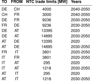
Table 3: Changes to NTC trade limitations between market zones in MW as modeled for all 2020-2050 simulations. These NTC replace those previous listed and are based on already planned cross border transmission expansions [3] and assumed longer-term enhancements.

TO FROM NTC trade limits [MW] Years

DE CH 4000 2040-2050

CH FR 3000 2040-2050

DE FR 9236 2030-2050

FR DE 9236 2030-2050

DE AT 13395 2020

DE AT 14895 2030-2050

AT DE 13395 2020

AT DE 14895 2030-2050

FR IT 3801 2020-2050

IT FR 3801 2020-2050

IT AT 295 2020

IT AT 1218 2030-2050

AT IT 295 2020

AT IT 1218 2030-2050

The Network Security and Expansion Module (Cascades) uses module specific data for the the under-frequency load shedding (UFLS) scheme, the under-voltage load shedding (UVLS) procedure, and to generate the sets of initial failures (contingencies). The Cascades module utilizes an UFLS scheme that is based on the Swissgrid transmission code 2013 [9]. Table 4 shows the UFLS actions undertaken by Cascades during under-frequency events. The table shows that all units are disconnected when the frequency goes below the 47.5 Hz threshold. This measure is also applied for frequency larger than 51.5 Hz. Furthermore, Cascades uses UVLS procedure to restore voltage below 0.92 p.u. For that purpose, at the buses where voltage violation is detected, a stepwise load shedding routine removes 25% of the load at each step until the voltage is restored. To generate the sets of contingencies we use only one failure probability for all lines and transformers in the system, with a default value of 0.001.

(14)

More on the Cascades UFLS scheme, UVLS procedure, and the generation of the contingencies can be found in the "Cascades Module Documentation" report.

Table 4: The UFLS data used in the Cascades module.

Frequency, f (Hz)

Action

Cumulative load shedded

(%) 49.8<f≥49.5 Activate reserves - 49.5<f≥49.0 Disconnect pumps - 49.0<f≥48.7 Disconnect pumps + Load shedding 15 48.7<f≥48.4 Disconnect pumps + Load shedding 25 48.4<f≥48.1 Disconnect pumps + Load shedding 40 48.1<f≥47.5 Disconnect pumps + Load shedding 60

f<47.5 Disconnect all units -

1.2 Distribution grid

Nexus-e represents the distribution grid on an aggregated cantonal level. Most data used for the distribution grid (e.g., wholesale prices and reserve requirements) are internally calculated within the Nexus-e framework. While we do not model the distribution grid, we connect the cantonal values (e.g., electricity load profiles) to the nodes of the transmission grid. The Investment loop exemplifies this cantonal-node connection: First, CentIv provides to Distributed Investments Module (DistIv) the nodal electricity load and wholesale prices, along with the Swiss reserve requirements. In turn, DistIv sums the nodal values for each canton and also calculates the cantonal wholesale prices using a weighted average of the prices of all nodes within each canton. The weights are defined as the ratio of the hourly nodal load to the hourly total load in each canton. Similarly, for the reserve requirements, we also use the weighted average. After DistIv identified the cost-optimal investments into distributed energy resources, it sends nodal residual demand and reserve requirements back to CentIv. To allocate the cantonal values to the multiple nodes in the canton, DistIv uses the same weights to disaggregate the cantonal value. Please note that while most cantons have multiple transmission nodes, six cantons have none. We include these cantons in nearby cantons with a transmission node¹.

As distribution transformers are rarely fully loaded in reality for security reasons, the power that is exchanged between the distribution and the transmission system considering the reserve provision is set to be limited by the transformer capacity, which is estimated by the regional peak demand multiplied by a factor of 1.2².

1Including data without transmission node into nearby cantons is necessary as input data such as network tariff, injection tariff and investment potentials of different resources are provided on a cantonal level.

2This means that for each region, the sum of the hourly net load and the hourly upward reserve minus the downward reserve should not be greater than 120% of the regional peak demand.

(15)

2 Electricity supply

A wide range of data are needed to implement realistic models of generators within a power system.

This section details the data used in Nexus-e to represent generators at the centralized (i.e., transmission system) level for Switzerland (Section 2.1) and the neighboring European Union (EU) countries (Section 2.2) as well as to represent generators at the distribution level of Switzerland (Section 2.3).

2.1 Swiss centralized generators

In this section, the necessary data and sources are presented for the Swiss generators located at the centralized level (i.e., transmission system level) of the energy system. These data include: the capacities and operating parameters (Section 2.1.1), the hydro inflow profiles and storage volumes (Section 2.1.2), the production profiles and placement for renewable energy source (RES) units (Sec- tion 2.1.3), the candidate unit capacities and placement (Section 2.1.4), and the generator costs along with fuel prices (Section 2.1.5).

2.1.1 Capacities and operating parameters

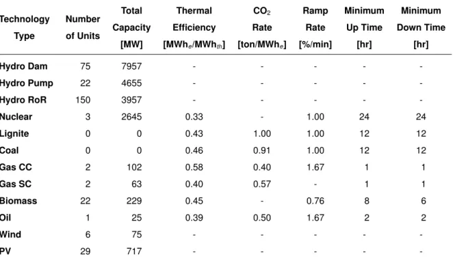
For existing Swiss generator capacities and locations, we use data from the Bundesamt für Energie (BFE) [10, 11, 12, 13] and previous studies [14]. Additionally, operational parameters for the different technology types are taken from available literature [15] as well as previous works [16]. Table 5 lists the operating parameters used for modeling the Swiss generation fleet along with the number of units and the total installed capacity for all units of each technology type. These parameters are used in the 2015 calibration simulation as well as the 2020-2050 scenario simulations. The total capacities listed represent those existing in 2020, which we assume also remain in place until 2050. For the 2015 calibration simulation, several hydro pump units are not included³because these units were commissioned between 2018 and 2019 and additional nuclear units are included⁴ since they were still operational in 2015.

The thermal efficiency, given in MWh of electricity (MWh_e) per MWh of thermal energy from fuel (MWh_th), represents the heat rate of the power plant and is used to quantify the fuel needed and associated fuel costs to produce any amount of electricity in MWh. Similarly, the CO₂rate, given in tons of CO₂ per MWh of electricity produced, represents the emission rate of the power plant and is used to quantify the CO₂costs to produce any amount of electricity in MWh. The ramp rate indicates how fast a generator can increase or decrease its level of electricity production and is given as a percentage of the generator’s rated capacity per minute. The minimum up and minimum down time indicate how many hours a unit must stay on or off once turned on or off. Blanks in these data indicate that the parameter does not apply to a technology type (e.g., there is no thermal efficiency for generators that do not con- sume fuel) or that the parameter is not constrained in the model (e.g., the ramp rate for a gas simple cycle (SC) generator is fast enough that it can easily reach its rated capacity in less than one hour).

Since we do not model the heating sector in Nexus-e, existing combined heat and power (CHP) units operate similar to normal gas-fired or oil-fired power generation units. We do not include carbon dioxide (CO₂) levy refund for gas-fired CHP plants. Furthermore, we do not include a market premium for hydro power.

In addition to these generators, a range of candidate units are modeled as potential investments.

3The new hydro pump units include: Limmern (2018), Nant de Drance (2019), and Veytaux (expanded in 2018).

4Both Beznau A and Muehleberg were still operational in 2015.

(16)

Table 5: Operating parameters for Swiss generators. Number of units and total capacities are for the 2020-2050 simulations (additional data for the nuclear phase-out can be seen in Section 7).

Technology Type

Number of Units

Total Capacity

[MW]

Thermal Efficiency [MWhe/MWhth]

CO2

Rate [ton/MWhe]

Ramp Rate [%/min]

Minimum Up Time

[hr]

Minimum Down Time

[hr]

Hydro Dam 75 7957 - - - - -

Hydro Pump 22 4655 - - - - -

Hydro RoR 150 3957 - - - - -

Nuclear 3 2645 0.33 - 1.00 24 24

Lignite 0 0 0.43 1.00 1.00 12 12

Coal 0 0 0.46 0.91 1.00 12 12

Gas CC 2 102 0.58 0.40 1.67 1 1

Gas SC 2 63 0.40 0.57 - 1 1

Biomass 22 229 0.45 - 0.76 8 6

Oil 1 25 0.39 0.50 1.67 2 2

Wind 6 75 - - - - -

PV 29 717 - - - - -

While the operating parameters for these units are the same as the values listed in Table 5, information regarding the number of units and total capacity by technology type can be found in Section 2.1.4.

For the outage periods of the Swiss nuclear reactors we used data from [17]. All Swiss nuclear reactors have a refueling outage every 12 months. Therefore, we assume that the planned refueling outages are occurring in the same period in all future scenario-years. Table 6 shows all modeled outages for each of the Swiss nuclear reactors in 2015 (second column) and the planed refueling outages for the reactors still operating in 2020 until the end of their lifetime (third column). The lifetime of the Swiss reactors depends on the simulated scenario (see Section 7).

Table 6: The outage schedules of Swiss nuclear reactors for the 2015 reference year and future scenario- years.

Reactor 2015 2020 - end of lifetime

Beznau 1 weeks 11-53 (43 weeks) weeks 17-20 (4 weeks) Beznau 2 weeks 32-50 (20 weeks) weeks 32-35 (4 weeks) Goesgen weeks 23-26 (4 weeks) weeks 22-25 (4 weeks) Leibstadt weeks 34-38 & 41-43 (8 weeks) weeks 23-26 (4 weeks) Muehleberg weeks 32-35 (4 weeks) not in operation

(17)

2.1.2 Hydro inflows and storage volumes

In addition to the parameters for hydro generators provided in Table 5, more input information is needed to represent the natural water inflows for all hydro generator types and the storage volumes of hydro dams and pumps.

For the hydro dam and pump units, an original hourly inflow profile is derived from the known monthly production [18] and weekly storage levels [19] of the Swiss hydro storage units (dams and pumps); a second original profile is derived using the known monthly production of Swiss hydro run of river (RoR) units [18]. Based on the Swiss hydro generator capacities, these profiles are scaled and applied to each hydro dam/pump and RoR unit in Switzerland as well as the aggregate units in the surrounding countries. The original hydro profiles are one of the input data parameters adjusted during the calibration process. After the initial simulations during the calibration, it was clear that these original profiles did not yield correct annual production from the non-Swiss hydro units; so, separate profiles are created for the surrounding country dams/pumps and RoR units to correctly reflect the expected annual production while maintaining the same hourly profile patterns of the original Swiss profiles. Additionally, it was evident that applying the same inflow profile to pumps and dams yielded only minimal use of pumping for charging (i.e., the natural water inflows to dams were so high that little pumping was necessary);

therefore, the Swiss and neighboring regions’ pump profiles are scaled down so the magnitudes of the discharging and charging from pump units reflect the historical data for each region closely. It is important to note that the process of creating realistic inflow profiles for Swiss hydro dams and pumps is complicated by the fact that historical data for these two generator types are always combined, even though these generator types tend to operate in very different cycles and behaviors. More on the hydro profile calibration can be found in the "Validation and Calibration of Modules" report.

In this work, the complex networks of cascading reservoirs and hydro generators that form the Swiss hydro generation fleet are not modeled in a high level of detail. Instead, we represent each hydro dam unit as being connected to an individual reservoir and each hydro pump unit as being connected to a single upper and single lower reservoir of equal sizes. To represent the volumes of these reservoirs, data are collected on the actual volumes of existing reservoirs and the elevation difference between the reservoir and the connected generator [12] to calculate the potential energy of the full reservoir.

For hydro pumps, we utilize these calculated energy volumes. However, because of the complexity of the cascades in Switzerland (e.g., some reservoirs are connected to multiple dam units), allocating an individual reservoir volume to each hydro dam is not straightforward. For this reason, a simpler approach is applied for hydro dams. To define an energy volume for each individual hydro dam, we assume that each reservoir is sized similarly and can provide continuous discharging for an extended period of time.

Since we know the total energy volume of all hydro dam and pump units in Switzerland in 2020 is around 8.85 TWh, and we already fix the hydro pump volumes based on the potential energy calculation (the sum of all pumps provide around 1.98 TWh), we can define a common length of continuous discharging time for all hydro dam units to achieve the desired Swiss total energy volume. To reach the 8.85 TWh, we define the energy volume of all hydro dam units such that they each can continuously discharge for 863 hours. This assumption also enables these dam units to follow the expected long-term (i.e., seasonal) behaviors.

All hydro storage units (dams and pumps) are set with a common starting and ending energy level for their reservoirs based on data from BFE on the historical weekly storage levels [19]. Since 2015 is used for the calibration, we also apply this year’s initial energy volume (i.e., 63%) for all 2020-2050 simulations. The known energy volume at the end of 2015 (46%) is applied for the 2015 calibration, while we set the ending volume equal to the starting volume (63%) for the 2020-2050 simulations.

(18)

2.1.3 Renewable production and placement

In addition to the parameters for wind and photovoltaic (PV) generators provided in Table 5, more input information is needed to represent their hourly production profiles and their placement within the Swiss transmission grid. Both of these additional inputs rely heavily on data available from previous works as part of the AFEM (Assessing Future Electricity Markets) project [14] that included detailed assessments of the RES potentials and generation profiles.

To represent the existing wind generators in Switzerland, capacity and location data are gathered from the BFE geodata platform for wind energy plants [12] for all moderately sized wind turbines (i.e., all installations with greater than 1.0 MW of wind capacity). The geographical location of these wind farms is used to define their electrical location within the Swiss transmission system; in most cases the wind capacity is placed at the nearest electrical node. The largest of these wind farms, Mt Crosin, is placed at the Bassecourt node based on feedback from Swissgrid. The hourly production profiles for these existing units are set based on a generation-weighted share of a scaled version of the AFEM 2015 Swiss hourly wind production profile [14]. The scaling is done to ensure that the total wind generation matches the historical total for the 2015 calibration year [20].

Additionally, to model potential future investments in wind farms at the centralized (transmission) level, the seven locations with the highest potential are identified from the detailed assessment con- ducted in the AFEM project [14]. In total, the capacities of these wind farms amount to nearly 2 GW with an annual production of almost 4 TWh. Since the locations for potential future wind farms are heavily restricted within Switzerland [21], these seven candidate locations are the only options included in the Nexus-e platform. The hourly production profiles for these candidate wind units are utilized from the previous work in AFEM.

To represent the existing PV generators in Switzerland, all locations providing at least 1% of the total Swiss PV production are identified from the AFEM assessment [14]. Twenty-nine locations are therefore selected along with the appropriate capacities for implementation in the Nexus-e platform. The hourly production profiles for these existing units are set based on a generation-weighted share of a scaled version of the AFEM 2015 Swiss hourly PV production profile [14]. The scaling is done to ensure that the total PV generation matches the historical total for the 2015 calibration year [20].

2.1.4 Candidate generators

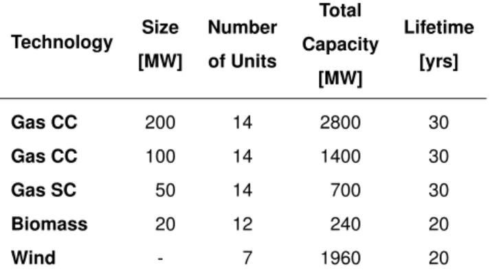
For centralized capacity expansion planning, we include candidate units for gas combined cycle (CC), gas SC, biomass, and wind, as shown in Table 7. The total candidate capacity for each technology type is based on potentials provided by [22, 23]. It is important to note that in accordance with these PSI reports [22, 23], investment costs for these centralized units are assumed constant throughout the scenario-years (see data related to gas-fired power plants in Figure 15.8 of [23] and discussions related to the uncertainty of wind costs in Section 7.3.1 [22] and Section 8.5.5 [23]). No investment subsidy is included to offset the investment costs for new gas-fired units. The costs of biomass reflect current waste incineration subsidies [22, 23], which we expect to continue in the future. The considered subsidies offset a large portion of the investment and operating costs for the candidate biomass units as well as the existing ones. We restrict the total candidate capacity of biomass to account for limited resource availability [22, 23]. We also limit the total candidate capacity of wind power to be in line with the review on the potential of wind power in Switzerland in [23]. Wind candidates are included that in total produce around 4.0 TWh/a, which is also consistent with the Swiss wind energy concept [24]. Due to the uncertainty of future cost projections of wind projects in Switzerland [22, 23], we assume constant investment costs in the period 2020-2050, but also include a sensitivity analysis of wind investments in the Scenario Results Report. The current production subsidy (KEV) is not included for wind candidate

(19)

units since KEV is scheduled to phase out in 2022 and it is unlikely any new wind turbines would get accepted into the KEV before then. We do not consider candidates for new hydro investments because of the need for extensive information about the location and costs for expansion of existing hydro or new hydro units. Therefore, we also do not include investment grants for hydro power. In the scope of this project, we do not include geothermal units as candidates, hence, we do not include subsidies for geothermal. The main reason for not including geothermal capacities was the high level of uncertainty regarding the potential and costs of this technology in Switzerland [22, 23]. Due to this uncertainty, the additional computational burden to simulate geothermal power plants and the researchers’ time required to set up all necessary parameters and locations for the candidate units was deemed too high.

It is important to note that we do not include candidate units in the neighboring countries and instead endogenously fix future capacities based on the 2016 EU reference scenario from PRIMES [25], as shown in Section 2.2.

Table 7: Data for candidate units at the transmission system level in Switzerland (2020–2050)

Technology Size [MW]

Number of Units

Total Capacity

[MW]

Lifetime [yrs]

Gas CC 200 14 2800 30

Gas CC 100 14 1400 30

Gas SC 50 14 700 30

Biomass 20 12 240 20

Wind - 7 1960 20

The gas candidate units are placed at system nodes with nuclear power plants where appropriate infrastructure exists (i.e. Beznau A, B, Muehleberg (220 kV) and Goesgen (380 kV)) or at locations where new developments were discussed (i.e Chavalon and Cornaux). We differentiate between different sizes of gas candidate units (50 MW / 100 MW / 200 MW) as shown in Table 7 as well as different technologies (Open/Combined Cycle). We also include multiple candidates of the same size at each system node. Candidate biomass units are located at the 6 substations with the largest power output from currently existing waste incineration power plants. As described in Section 2.1.3, for large-scale wind installations, the placement of candidate units is based on the seven locations with the highest wind potential determined in AFEM [14].

2.1.5 Generator costs and fuel prices

To represent the variable operating costs of all Swiss generators (existing and candidates) along with the investment and fixed costs associated with building a new generator in Switzerland (candidates only) we use data from recent BFE sponsored studies [22, 23]. Table 8 lists these costs by technology type.

The costs of biomass reflect current waste incineration subsidies [22, 23], which we expect to continue in the future. It is important to note that we assume constant investment costs and fixed costs throughout the scenario-years for the candidate units. Similarly the VOM cost for each technology type is the same in the 2015 calibration year and in the 2020-2050 scenario-years; however, the fuel and CO2portions of the total variable operating cost will change based on the assumed trajectories for the prices of each fuel and the price of CO2in future years. Table 9 lists the fuel prices and CO2price for the 2015 reference year, which were provided by [22, 23], and the prices for the 2020-2050 scenario-years, which were adopted from the 2016 EU reference scenario data in [25].

(20)

Table 8: Cost parameters for Swiss generators. Variable operation and maintenance (VOM) cost is used for the 2015 and 2020-2050 simulations. Fixed operation and maintenance (FOM) and investment costs are used for the candidate units in the 2020-2050 simulations.

VOM Cost [EUR/MWh]

FOM Cost [kEUR/MW/a]

Investment Cost [kEUR/MW/a]

Hydro Dam 11.0 - -

Hydro Pump 9.0 - -

Hydro RoR 9.5 - -

Nuclear 20.0 - -

Gas CC 16.2 25.0 58.5

Gas SC 12.1 18.0 36.1

Biomass 1.0 0.0 124.8

Oil 80.0 - -

Wind 2.5 45.4 182.4

PV 2.7 - -

In all years, the Swiss prices for CO2 are the same as the CO2 prices applied to the neighboring country generators. For the 2015 calibration year, these Swiss fuel prices are unique compared to the prices set for all other EU generators, shown in Table 17. However, in the 2020-2050 scenario-years, the Swiss and EU fuel prices for natural gas, oil, and uranium are kept equal to maintain consistency with the assumptions, also taken from the 2016 EU reference scenario, for the neighboring country capacity development from 2020 to 2050 [25]. However, the prices in Switzerland for biomass are unique compared to the neighboring country generators, which reflects the current Swiss waste incineration subsidies [22, 23].

Table 9: The fuel prices (EUR/MWh_th) and CO₂ price (EUR/ton) for Swiss generators for the 2015 calibration year and the 2020-2050 scenario-years.

Fuel [EUR/MWhth] and CO2[EUR/ton] Prices Fuel 2015 2020 2030 2040 2050 Gas 25.3 32.9 40.1 44.3 45.9 Oil 41.5 51.2 66.2 73.2 76.6 Biomass 0.0 0.0 0.0 0.0 0.0 Uranium 1.4 3.0 3.0 3.0 3.0 CO2 8.0 15.0 33.5 50.0 88.0

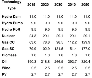
Using the VOM costs provided in Table 8 and combining the generator parameters in Table 5 with the fuel and CO₂prices in Table 9, the total variable operating costs for Swiss generators of each technology type can be calculated for any of the years simulated. Table 10 shows these total variable operating costs for each technology type in each of the years simulated. Comparing the different Swiss technologies, renewable units provide the lowest cost electricity (i.e., biomass, wind, and PV), followed by hydro units that also have quite low operating costs (i.e., hydro pumps, RoRs, and dams). Nuclear power provides

(21)

electricity at the next lowest cost, followed by the other conventional generator types (gas CC and gas SC), leaving the oil as the most expensive generator type in Switzerland. From 2020 to 2050, while the RES, hydro, and nuclear units have consistent total variable costs, the contributions from the fuel and CO₂costs result in steady increases to the Swiss gas and oil generator types until 2050.

Table 10: The total variable costs for Swiss generators for the different years simulated. This total variable cost is a combination of the VOM cost, fuel cost, and CO2cost.

Total Variable Cost [EUR/MWh]

2015 2020 2030 2040 2050

Hydro Dam 11.0 11.0 11.0 11.0 11.0 Hydro Pump 9.0 9.0 9.0 9.0 9.0

Hydro RoR 9.5 9.5 9.5 9.5 9.5

Nuclear 24.3 29.1 29.1 29.1 29.1 Gas CC 63.0 78.8 98.5 112.2 129.9 Gas SC 79.9 102.9 131.5 151.4 177.0

Biomass 1.0 1.0 1.0 1.0 1.0

Oil 190.3 218.8 266.5 292.7 320.4

Wind 2.5 2.5 2.5 2.5 2.5

PV 2.7 2.7 2.7 2.7 2.7

2.2 European generators

In this section, the necessary data and sources are presented for the neighboring EU generators located at the centralized level (i.e., transmission system level) of the energy system. These data include:

the capacities and operating parameters (Section 2.2.1), the hydro inflow profiles and storage volumes (Section 2.2.2), the production profiles for RES units (Section 2.2.3), and the generator costs along with fuel prices (Section 2.2.4).

All generators in the neighboring EU countries are aggregated to one unit per technology type. Much of the data needed to represent these EU generator capacities are adopted from the PRIMES 2016 EU reference scenario data in [25]. Additionally, the EU generator parameters (VOM costs, CO2rates, and efficiencies) are based on the information provided in the “Current and Prospective Costs of Electricity Generation until 2050” prepared and published by the DIW Berlin [15]. This document comprises data from different sources, and those that we used most frequently are:

• IEA, NEA, & OECD, Projected Costs of Generating Electricity [26, 27]

• IPCC, Renewable Energy Sources and Climate Change Mitigation [28, 29]

• IRENA, Biomass for Power Generation [30]

2.2.1 Capacities and operating parameters

For the 2015 calibration, the generator capacities are defined using data from ENTSO-E [31]. In all 2020- 2050 scenarios, the generator capacities are instead defined based on the installed capacity projections

(22)

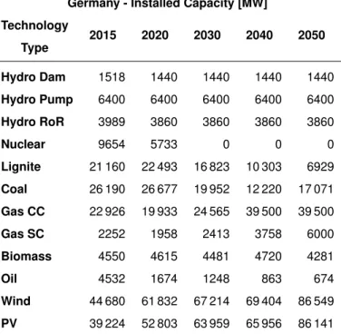
from the 2016 EU reference scenario [25]. Tables 11, 12, 13, and 14 provide the values for the capacities by technology type over the simulated years for each of the four neighboring countries. As part of the calibration process, some of the capacities listed have been adjusted. For instance, to achieve agreement with the annual production totals for these aggregate units, we apply capacity factors to some technology types to reduce their available capacity over the full year (for Nuclear: DE=83% &

FR=85%; for Biomass: DE=65% & IT=50%). The generator capacities of each surrounding country are placed at the main country node (not at the border node).

Table 11: German generators are represented by single units aggregated by technology type. Capacities change over time based on data provided in [25].

Germany - Installed Capacity [MW]

2015 2020 2030 2040 2050

Hydro Dam 1518 1440 1440 1440 1440 Hydro Pump 6400 6400 6400 6400 6400 Hydro RoR 3989 3860 3860 3860 3860

Nuclear 9654 5733 0 0 0

Lignite 21 160 22 493 16 823 10 303 6929 Coal 26 190 26 677 19 952 12 220 17 071 Gas CC 22 926 19 933 24 565 39 500 39 500

Gas SC 2252 1958 2413 3758 6000

Biomass 4550 4615 4481 4720 4281

Oil 4532 1674 1248 863 674

Wind 44 680 61 832 67 214 69 404 86 549 PV 39 224 52 803 63 959 65 956 86 141

The operating parameters for the aggregate generators of all the neighboring countries are the same as those shown for the Swiss generators in Table 5; however, the ramp rate and minimum up/down time are not applied to these units since they are aggregated representations of many generators and would not be expected to match these operating limitations.

(23)

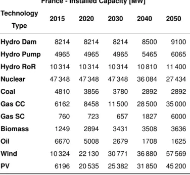
Table 12: French generators are represented by single units aggregated by technology type. Capacities change over time based on data provided in [25].

France - Installed Capacity [MW]

2015 2020 2030 2040 2050

Hydro Dam 8214 8214 8214 8500 9100 Hydro Pump 4965 4965 4965 5465 6065 Hydro RoR 10 314 10 314 10 314 10 810 11 400 Nuclear 47 348 47 348 47 348 36 084 27 434

Coal 4810 3856 3780 2892 2892

Gas CC 6162 8458 11 500 28 500 35 000

Gas SC 760 723 657 1827 6000

Biomass 1249 2894 3431 3508 3636

Oil 6670 5008 2679 1708 1625

Wind 10 324 22 130 30 771 36 880 57 569

PV 6196 20 535 25 382 31 850 45 200

Table 13: Italian generators are represented by single units aggregated by technology type. Capacities change over time based on data provided in [25].

Italy - Installed Capacity [MW]

2015 2020 2030 2040 2050

Hydro Dam 6362 4733 4733 4733 4733 Hydro Pump 4714 6453 6453 6453 6453 Hydro RoR 10 719 10 826 10 826 10 826 10 826

Coal 8800 8858 5098 2226 3802

Gas CC 50 140 49 473 40 212 43 559 86 826

Gas SC 1904 1879 1527 1654 3298

Biomass 2405 2694 2705 3076 3057

Oil 8800 8629 2332 603 128

Wind 9200 10 700 15 577 17 736 25 957 PV 18 900 20 400 24 562 27 050 56 765

(24)

Table 14: Austrian generators are represented by single units aggregated by technology type. Capacities change over time based on data provided in [25].

Austria - Installed Capacity [MW]

Technology

Type 2015 2020 2030 2040 2050

Hydro Dam 4254 4449 4450 4491 4543 Hydro Pump 2971 3401 3401 3674 3717 Hydro RoR 5543 5662 5664 5716 5782

Coal 1171 804 778 72 36

Gas CC 4501 3527 2902 3046 2850

Biomass 608 778 813 1033 846

Oil 178 178 178 8 0

Wind 2404 2887 4545 5026 6803

PV 489 1193 282 2930 4009

2.2.2 Hydro inflows and storage volumes

In addition to the installed capacities of hydro generators provided in Tables 11-14, more input information is needed to represent the natural water inflows for all hydro generator types and the storage volumes of hydro dams and pumps. More details on the definition of these parameters is provided in Section 2.1.2.

Separate inflow profiles are created for the surrounding country dams, pumps, and RoR units to correctly reflect their expected annual production while maintaining the same hourly profile patterns of the original Swiss profiles. Similar to the modeling of Swiss hydro storages, we represent each aggregated hydro dam unit as being connected to an individual reservoir and each hydro pump unit as being connected to a single upper and single lower reservoir of equal sizes. To represent the volumes of these reservoirs, a simple approach equivalent to what was used for the Swiss hydro dams is applied.

However, for these non-Swiss aggregate units, we define a common length of continuous discharging time for both hydro dam and hydro pump units. Each dam reservoir is sized to be able to continuously discharge for 863 hours, while each pump unit’s upper and lower reservoir are sized to be able to continuously discharge for 100 hours. These sizes enable the dam and pump units to operate in the typical seasonal (dam) and daily (pump) patterns.

2.2.3 Renewable production

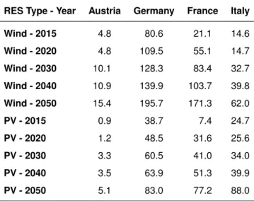
In addition to the capacities for wind and PV generators provided in Tables 11-14, more input information is needed to represent their hourly production profiles. Creating these profiles relies heavily on data available from previous works as part of the AFEM project [14] that included detailed assessments of these RES potentials and generation profiles.

The hourly production profiles for the wind and PV units are set based on scaling a version of the AFEM hourly wind and PV production profiles for each country in each year [14]. The scaling is done to ensure that the annual production matches the historical total for each year. Different data sources are utilized for the annual totals in the neighboring countries. For the 2015 calibration simulation, various

(25)

data sources provide annual total production for wind or PV in the four neighboring countries [32, 33, 34, 35, 31, 14]. For the 2020-2050 scenario-years, the PRIMES 2016 EU reference scenario [25] is the only source used to set the annual production totals for wind and PV in each of the neighboring countries.

Table 15 lists the annual totals for wind and PV in each year for the neighboring countries. Once scaled, the hourly profiles are applied in the Nexus-e platform for the corresponding neighboring country in the appropriate year.

Table 15: The annual wind and PV production (TWh) of the units located in the Swiss neighboring countries for each simulated year.

RES Type - Year Austria Germany France Italy

Wind - 2015 4.8 80.6 21.1 14.6

Wind - 2020 4.8 109.5 55.1 14.7

Wind - 2030 10.1 128.3 83.4 32.7 Wind - 2040 10.9 139.9 103.7 39.8 Wind - 2050 15.4 195.7 171.3 62.0

PV - 2015 0.9 38.7 7.4 24.7

PV - 2020 1.2 48.5 31.6 25.6

PV - 2030 3.3 60.5 41.0 34.0

PV - 2040 3.5 63.9 51.3 39.9

PV - 2050 5.1 83.0 77.2 88.0

2.2.4 Generator costs and fuel prices

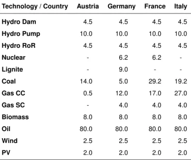
To represent the variable operating costs of all EU generators, we use data from the comprehensive review done by [15]. Table 16 lists these cost by technology type for each of the Swiss neighboring countries modeled by the Nexus-e platform. Note that, several VOM costs were adjusted as part of the calibration process of the CentIv and eMark modules⁵.

The VOM cost for each technology type is the same in the 2015 calibration year and in the 2020-2050 scenario-years; however, the fuel and CO2portions of the total variable operating cost will change based on the assumed trajectories for the prices of each fuel and the price of CO2in future years. Table 17 lists the fuel prices and CO2price for the 2015 reference year, which were provided by [15], and the prices for the 2020-2050 scenario-years, which were adopted from the 2016 EU reference scenario data in [25].

In all years, the prices assumed for CO2are the same in Switzerland and in the neighboring countries.

For the 2015 calibration year, these neighboring EU fuel prices are unique compared to the prices set for the Swiss generators, shown in Table 9. However, in the 2020-2050 scenario-years, the Swiss and EU fuel prices for natural gas, oil, and uranium are kept equal to maintain consistency with the assumptions for the neighboring country capacity development from 2020 to 2050, which are also taken from the 2016 EU reference scenario [25].

Using the VOM costs provided in Table 16 and combining the generator parameters in Table 5 with the fuel and CO2prices in Table 17, the total variable operating costs for generators of each technology type in the neighboring countries can be calculated for any of the years simulated. Tables 18 and 19

5For more information regarding the calibration of the CentIv and eMark modules the reader is referred to the "Validation and Calibration of Modules" report.

(26)

Table 16: The VOM costs (EUR/MWh) of the units located in the Swiss neighboring countries.

Technology / Country Austria Germany France Italy

Hydro Dam 4.5 4.5 4.5 4.5

Hydro Pump 10.0 10.0 10.0 10.0

Hydro RoR 4.5 4.5 4.5 4.5

Nuclear - 6.2 6.2 -

Lignite - 9.0 - -

Coal 14.0 5.0 29.2 19.2

Gas CC 0.5 12.0 17.0 27.0

Gas SC - 4.0 4.0 4.0

Biomass 8.0 8.0 8.0 8.0

Oil 80.0 80.0 80.0 80.0

Wind 2.5 2.5 2.5 2.5

PV 2.0 2.0 2.0 2.0

Table 17: The fuel prices (EUR/MWh_th) and CO2price (EUR/ton) for the neighboring country generators for the 2015 reference year and the 2020-2050 scenario-years.

Fuel [EUR/MWhth] and CO2[EUR/ton] Prices Fuel 2015 2020 2030 2040 2050 Gas 21.0 32.9 40.1 44.3 45.9 Coal 8.5 9.8 14.5 16.0 17.0 Lignite 5.1 4.4 4.4 4.4 4.4 Oil 31.8 51.2 66.2 73.2 76.6 Biomass 3.4 7.2 7.2 7.2 7.2 Uranium 3.0 3.0 3.0 3.0 3.0 CO2 8.0 15.0 33.5 50.0 88.0

(27)

below provide demonstrations of these total variable operating costs for 2020 and 2050, respectively.

Table 18: The total variable costs (EUR/MWh) for the units located in the Swiss neighboring countries in the 2020 scenario-year.

Hydro Dam 4.5 4.5 4.5 4.5

Hydro Pump 10.0 10.0 10.0 10.0

Hydro RoR 4.5 4.5 4.5 4.5

Nuclear - 15.3 15.3 -

Lignite - 34.2 - -

Coal 49.0 40.0 64.1 54.1

Gas CC 60.9 72.4 77.4 87.4

Gas SC - 98.4 98.4 98.4

Biomass 24.0 24.0 24.0 24.0

Oil 218.8 218.8 218.8 218.8

Wind 2.5 2.5 2.5 2.5

PV 2.0 2.0 2.0 2.0

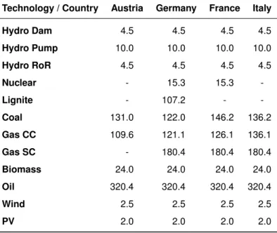
Table 19: The total variable costs (EUR/MWh) for the units located in the Swiss neighboring countries in the 2050 scenario-year.

Hydro Dam 4.5 4.5 4.5 4.5

Hydro Pump 10.0 10.0 10.0 10.0

Hydro RoR 4.5 4.5 4.5 4.5

Nuclear - 15.3 15.3 -

Lignite - 107.2 - -

Coal 131.0 122.0 146.2 136.2

Gas CC 109.6 121.1 126.1 136.1

Gas SC - 180.4 180.4 180.4

Biomass 24.0 24.0 24.0 24.0

Oil 320.4 320.4 320.4 320.4

Wind 2.5 2.5 2.5 2.5

PV 2.0 2.0 2.0 2.0

2.3 Swiss distributed generators

The modeled distribution system consists of six types of distributed energy technologies, namely PV, biomass wood, biomass manure, CHP, grid-battery, and PV-battery. Grid-batteries charge during low electricity price periods and discharge during high electricity price periods to make inter-temporal market

(28)

arbitrage. PV-batteries have no direct connection to the grid and in general charge (discharge) when the demand of the PV investor is lower (higher) than his PV generation. Table 20 provides an overview of key parameters for these technologies, using 2018 as the reference year (if not specified otherwise). For the distributed generation technologies we use the data from [23], while for grid-battery and PV-battery, we use the information on the Tesla Powerpack and Powerwall 2 [36]. We assume that PV-batteries have a ratio of 13.5 kWh to 5kW, meaning that a 27 kWh battery has a capacity of 10 kW. This ratio is based on the Tesla Powerwall 2. PV-batteries are continuously sized, meaning that they can have every size, but they utilize the above mentioned ratio between size (kWh) and capacity (kW). We choose continuous sizing because we consider PV-battery investments on a cantonal level. Furthermore, we do not include any subsidies for batteries. The total cost of installing Tesla Powerwall 2 is calculated assuming that the battery pack costs available on [36] account for 46% of the total investment costs [37]. We include decreasing investment and operation costs for PV and batteries until 2050, while all other parameters remain constant. The current production subsidy (KEV) is not included for the PV candidate units since KEV is scheduled to phase out in 2022 and it is unlikely any new PV would get accepted into the KEV before then. Table 21 presents the assumptions on the development of PV and storage investment and operation costs, presented in percentage of the reference year 2018 based on [23].

Table 20: Parameters for candidate units

Type Size

Investment cost (EUR/kW)

Variable operation

cost (cent/kWh)

Fixed operation

cost (EUR/kW/year)

Fuel cost (cent/kWh)

Emissions (eq. g/kWh)

Lifetime (years)

Amortization period (years)

PV 0-10 kWp 2’902 2.73 0 0 0 30 10

PV 10-30 kWp 2’295 2.73 0 0 0 30 10

PV 30-100 kWp 1’570 2.73 0 0 0 30 10

PV >100 kWp 1’182 1.82 0 0 0 30 10

Biomass

wood 50 kWe 6’033 0 675 19.00 35 10 10

Biomass

manure 25 kWe 32’909 0 968 8.64 0 15 15

CHP 10 kWe 4’127 3.50 0 7.59 611 20 20

Grid-connected

battery 100 kWh 638 0 2.5% of

investment cost 0 0 20 20

PV-battery 13.5 kWh 1’156 0 2.5% of

investment cost 0 0 15 15

Table 21: Assumptions for future investment and operational costs.

(a) Investment costs

Category 2018 2020 2030 2040 2050

PV 0-10 kWp 100% 86% 71% 61% 57%

PV 10-30 kWp 100% 87% 71% 57% 44%

PV 30-100 kWp 100% 84% 69% 57% 48%

PV >100 kWp 100% 81% 66% 57% 52%

Grid-connected

battery 100% 100% 72% 53% 39%

PV battery 100% 100% 72% 53% 39%

(b) Operational costs

Category 2018 2020 2030 2040 2050

PV 0-10 kWp 100% 95% 78% 68% 64%

PV 10-30 kWp 100% 95% 78% 68% 64%

PV 30-100 kWp 100% 95% 78% 68% 64%

PV >100 kWp 100% 95% 78% 68% 64%

Grid-connected

battery 100% 100% 72% 53% 39%

PV battery 100% 100% 72% 53% 39%

We include four PV categories (i.e., 0-10 kWp, 10-30 kWp, 30-100 kWp, >100 kWp) and limit the maximum installed capacity for each category according to its PV potential, which we calculated based on the Sonnendach data [38] assuming the area required for 1 kWp of PV is 6 square-meters. PV

(29)

potentials in Switzerland are shown in Figure 2 and Figure 3. Not all cantons are shown in Figure 2 as PV potentials of cantons without transmission nodes are aggregated into the nearby cantons. For PV electricity generation, we use irradiation data from MeteoSwiss [39]. We assume a linear degradation rate of 0.5% per year for PV panels (i.e., each year the annual PV output decreases by 0.5%) [40].

Details of the grid tariff, PV injection tariff and the wholesale-to-retail price margin that are used to model profitability of PV investments can be found in Section 5.

Figure 2: PV investment potential for different regions in MW.

For the investment potential of biomass technologies, we use the data from [23]. We do not limit the investment potential for CHP. In the investment decision for CHP units, we include their carbon emissions and the respective costs due to the CO₂ levy. However, we do not consider the CO₂ levy refund. Furthermore, no investment subsidy is included to offset the investment costs for new CHP. We do not include self-consumption of CHPs and, instead, assume that CHP owners sell the electricity at the wholesale market. We do so, as we assume that larger investors install CHP units and not individual households. For biomass wood/manure and CHP units, we assume a capacity factor of 0.54, 0.78, and 0.28 [23], respectively. These dispatchable generation units have a ramp rate limit of 25% of their maximum capacity per hour. Technical parameters of the candidate battery units are in Table 22.

Table 22: Technical parameters for candidate storage units.

Type Capacity

(kWh)

Maximum charging discharging power (kW)

Initial storage level (kWh)

Hourly self-discharging

rate (%)

Lifetime (years)

PV-battery 13.5 5 0 0 15

Grid-connected

battery 100 50 0 0.1 20

(30)