Volume 36, Issue 4

Volume 36, Issue 4

The role of the marginal rate of substitution of wealth for a loss averse investor

Jaroslava Hlouskova

Financial Markets and Econometrics, Institute for Advanced Studies, Vienna, Austria

Panagiotis Tsigaris

Department of Economics, Thompson Rivers University

Abstract

The marginal rate of substitution and the relative prices of goods have been used in economics to explain household's behavior but they have not been used yet in the behavioral economics literature. This note attempts to fill the gap in the literature with an application to a loss averse investor's demand for a risky asset in a one period model.

​E-mail Addresses: Jaroslava Hlouskova is a Senior Research Associate and can be reached at hlouskov@ihs.ac.at and Panagiotis Tsigaris is a Professor and can be reached at ptsigaris@tru.ca. J. Hlouskova is also affi​liated with the Department of Economics, Thompson Rivers University, Kamloops,BC, Canada and with the Ecosystems Services and Management at the International Institute for Applied Systems Analysis, Austria. The authors acknowledge the thoughtful comments and suggestions of the anonymous referee and of Ines Fortin. J.

Hlouskova gratefully acknowledges the support of Austrian Science Fund (FWF): project number V 438-N32.

Citation: Jaroslava Hlouskova and Panagiotis Tsigaris, (2016) ''The role of the marginal rate of substitution of wealth for a loss averse investor'', Economics Bulletin, Volume 36, Issue 4, pages 2250-2260

Contact: Jaroslava Hlouskova - hlouskov@ihs.ac.at, Panagiotis Tsigaris - ptsigaris@tru.ca.

Submitted: June 09, 2014. Published: November 27, 2016.

1 Introduction

The marginal rate of substitution (MRS) and the relative prices of goods are used in eco- nomics to explain investor’s behavior but these important concepts have not been applied yet in the behavioral economics literature (Thaler 2016).

The aim of this note is to fill this gap in the literature.

This is achieved by considering a one-period model for three types of loss averse investors based on the gross return from investing all initial wealth in the safe asset being (i) above the reference level, (ii) equal to the reference level and (iii) below the reference level.

Having low reference levels as in (i) could be driven by a self-enhancement or a feel good motive. An example, would be when the investor compares her wealth with other investors that are less successful in the stock market than she is. The investor feels good by doing comparisons with less fortunate market participants. On the other hand, a reference level equal to the gross return from the safe asset as in (ii) indicates for example the case where the investor compares with others that are as successful as the investor. Finally, having a high reference level as in (iii) can be due to the self-improvement motive (i.e, high aspirations).

For example, the investor compares her initial wealth to the initial wealth of another more successful investor. The investor wants to self-improve and possible reach and exceed the wealth of the successful investor.

Within this set-up we explore the effect of the loss aversion and the reference level on the MRS and hence on the optimal choice of risk taking. The summary of our findings is as follows.

Under case (i) we find that the MRS increases with decreased risk-taking as in expected utility models. It also increases with a decrease in the reference level. Furthermore, the investor by being sufficiently loss averse causes her MRS to be independent of the loss aversion parameter. As a result, risk taking is negatively related to the reference level and independent of loss aversion. Thus, under stated conditions the investor participates in the stock market.

For case (ii) a critical reference level, the MRS is independent of risky asset holdings.

Here the MRS depends inversely on the loss aversion parameter but is independent of the reference level. In terms of the optimal solution, the investor will not invest in a risky asset if the MRS is below the market trade-off of risky wealth even if the expected return of the risky asset exceeds the risk free rate. This can provide an explanation why a sizeable amount of people do not own stocks (Haliassos and Bertaut 1995) in the presence of a large equity premium (Mehra and Prescott 1985).

The loss aversion parameter plays an important role for MRS to be below the market trade-off. If it exceeds certain threshold then the investor will not participate in risk taking. Furthermore, any exogenous driven changes to the reference level could cause the investor to consider the other two cases.

Finally, in case (iii) the MRS increases when risk taking decreases as in the expected

1

The MRS is the slope of an individual’s indifference curve between wealth in the good and the bad state of nature (Stiglitz 1969). It shows the maximum willingness to pay to have an additional unit of wealth in the good state of nature by increasing investment in the risky asset while holding expected utility constant.

2

For prospect theory explanation see Gomes (2005), Bernard and Ghossoub (2010), and He and Zhou (2011).

3

See Falk and Knell (2004) and Hlouskova and Tsigaris (2012).

4

For alternative explanations of non-participation in the stock market see Barberis et al. (2006), Christelis

et al. (2010), van Rooij et al. (2011) and Berk and Walden (2013).

utility model and in the low reference level leading to an interior (closed form) solution.

However, in this scenario the MRS increases when the loss aversion parameter decreases and it increases when the investor’s reference level increases. For sufficiently loss averse investor the optimal solution indicates that an increase in reference levels (aspirations) will lead to more risk taking while in the low reference level the investor undertakes more risk taking with lower reference levels. In addition, the strictly positive investment in the risky asset decreases with increasing degree of loss aversion.

In the next section the model is described. Section 2.1 discusses low reference levels.

Section 2.2 analyzes critical reference levels. Section 2.3 explores high reference levels. Con- cluding remarks are given in section 3.

2 Portfolio decisions with loss aversion

Consider an investor who is deciding to allocate initial wealth, W

> 0, toward a risk free investment in the amount of m and a risky investment in the amount of a. The safe asset yields a net of the dollar investment return r > 0 and two states of nature determine the return of the risky asset, x ∈ {x

, x

}. In the good state of nature, the risky asset yields a net of the dollar investment return x

> 0 with probability p and in the bad state of nature it yields x

with probability 1 − p.

Furthermore, the rates of returns of the two assets are assumed to be such that x

< r < x

.

The terminal wealth W

is determined as

W

= (1 + r + (x

− r)α) W

, i ∈ {b, g} (1) where α =

is the proportion of initial wealth invested in the risky asset. We assume also that the proportion of wealth invested in the risky asset is within the interval 0 ≤ α ≤ α

≡

1+r

r−xb

for final wealth to be non-negative and short-selling being eliminated.

The loss aversion is modeled by introducing a typical Kahneman and Tversky (1979) utility function with loss aversion parameter λ > 1 given as follows

U

(W

− Γ) =



 

 

U

(W

− Γ) =

, W

≥ Γ λU

(W

− Γ) = −λ

, 0 ≤ W

< Γ

where Γ > 0 is a reference level of wealth. The loss aversion parameter λ captures the fact that investors are more sensitive when they experience an infinitesimal loss in financial wealth than when experiencing a similar size relative gain. The γ parameter determines the curvature of the utility function for relative gains and losses. We assume that γ ∈ (0, 1) in order to be consistent with the experimental findings of Tversky and Kahneman (1992).

Finally, it is easy to see that in the domain of relative gains, W

≥ Γ, the investor displays risk aversion, while in the domain of relative losses, W

< Γ, the investor is a risk lover.

Thus,

5

Similarly as Barberis and Huang (2001), Barberis et al. (2001), Berkelaar et al. (2004), De Giorgi (2011)

and Gomes (2005), we do not consider distorted (subjective) probabilities.

Max

: V = E (U

(W

− Γ)) = E (U

(λ, Γ, α)) such that : W

= [1 + r + (x

− r)α]W

, i ∈ {b, g}

0 ≤ α ≤ α







(2) In the following definitions we introduce the MRS and its market value.

Definition 1 The marginal rate of substitution (MRS) is the absolute value of the rate at which an investor gives up wealth relative to the reference level in the bad state of nature to gain an extra unit of wealth relative to the reference level in the good state of nature while maintaining the same level of the expected utility, E (U

(W

− Γ)). I.e.,

M RS = M RS(α, λ, Γ) =

d(W

− Γ) d(W

− Γ)

Definition 2 The market value of one unit of the relative wealth in the good state of nature equals to

units of relative wealth in the bad state of nature.

The following threshold parameter will be used later K

= (1 − p)(r − x

)

p (x

− r)

(3)

2.1 Low reference levels: Γ < (1 + r)W ₁

Reference levels below the gross return from investing the initial wealth in the safe asset can make the investor feel good. For example, the investor could be comparing her initial wealth level invested in the safe asset, (1 + r)W

, with other investors who have a lower initial wealth invested in the safe asset, (1 + r)W

where W

< W

, in order to feel good (self-enhancement). The investor could be comparing to someone who was not as successful in the financial market in the previous period.

Proposition 1 states the optimal risk taking under this case:

Proposition 1 For 0 < Γ < (1 + r)W

, λ > max{1, 1/K

} and E (x) > r it is optimal for a loss-averse investor to allocate a positive proportion (of her initial wealth) in the risky asset such that

α

= 1 − K

K

(x

− r) + r − x

(1 + r)W

− Γ W

(4) where MRS(α

, λ, Γ) =

and 0 < α

<

b)W1

. Proof. See Appendix.

The optimal solution shows, amongst other typical features, that a decrease in the refer-

ence level increases the proportion invested in the risky asset. Also the proportion invested

in the risky asset is independent of loss aversion.

Assuming the investor is sufficiently loss averse, i.e., λ > max{1, 1/K

}, she will select the proportion invested in the risky asset in such a way as to avoid relative losses in the bad state of nature as in problem (P2) defined in Appendix. The optimal solution is found in problem (P1) (see Appendix) where wealth in both states of nature, good and bad, is above the reference level. The MRS for a loss-averse investor defined by (2) with Γ < (1 + r)W

and in the region where the optimal investment occurs, 0 ≤ α ≤

b)W¹

, is M RS = M RS(α, Γ) = p

1 − p

−(r − x

)W

α + (1 + r)W

− Γ (x

− r)W

α + (1 + r)W

− Γ

(5) (see the proof of Proposition 1 in Appendix). The MRS increases as the proportion invested in the risky asset decreases. The MRS also increases as the reference level decreases. Hence, the economic intuition behind the increase in the proportion invested in the risky asset given a decrease in the reference level is the increase in the investor’s willingness to pay to add risk to her portfolio, i.e., the increase in the MRS. Furthermore, even though the investor needs to be sufficiently loss averse, to arrive to the optimal solution, the MRS is independent of the loss aversion parameter and hence not part of the optimal solution.

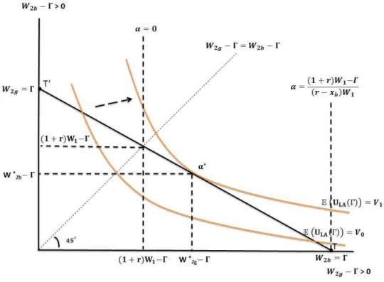
The investor’s optimal solution (4) is found by equating the investor’s valuation, as given by the MRS, of an additional unit of wealth in the good state of nature (net of the reference level) to the price of an additional unit of wealth in the good state of nature (net of the reference level). If M RS >

M RS <

along the budget line, the investor will increase (decrease) risky assets in order to increase (decrease) wealth in the good state of nature net of the reference level which reduces (increase) MRS until M RS(α

, λ, Γ) =

. Figure 1 illustrates the optimal solution.

2.2 Critical reference level: Γ = (1 + r)W 1

A reference level that coincides with the gross return from investing all initial wealth in the safe asset reflects a critical level. This could be because a loss averse investor compares with others that have similar initial wealth.

The marginal rate of substitution for a loss-averse investor defined by (2) with critical reference level such that Γ = (1 + r)W

is

M RS = M RS(λ) = p 1 − p

r − x

x

− r

1

λ if 0 < α ≤ α

(6)

(see the proof of Proposition 2 in Appendix). Contrary to expected utility models and the low reference level in the previous section, the marginal rate of substitution is not a continuous strictly decreasing function of the proportion allocated to the risky asset but is independent of it. This occurs because the reference level is set equal to the gross return of the safe asset as is done in many studies (see, e.g., Gomes 2005, Bernard and Ghossoub 2010, and He and Zhou 2011). The investor has no surplus wealth to allocate to the risky asset as seen also in (4).

In this situation, the marginal rate of substitution will be negatively affected by loss

aversion. As the investor becomes more (less) loss averse, i.e., λ increases (decreases), the

marginal rate of substitution to give up relative wealth in the bad state of nature for an extra

Figure 1: Low reference level: Γ < (1 + r)W

unit of relative wealth in the good state decreases (increases). The investor’s willingness to pay to undertake risky investment drops (increases) as λ increases (decreases), while keeping expected utility constant.

Let us introduce the following threshold probability p

= (r − x

)

(r − x

)

+ (x

− r)

(7)

A loss averse investor will either not participate in the stock market or put the maximum pos- sible in the risky asset as described in the following proposition. In the following proposition and discussions we consider M RS for α ∈ (o, α

].

Proposition 2 It is optimal for a loss averse investor, with the reference level being invest- ment in the safe asset, not to invest in the risky asset if the marginal rate of substitution is lower than the relative price of wealth in the good state of nature in terms of the bad state of nature, i.e., M RS <

. If M RS >

and p > p

then the investor will continue investing all of her initial wealth into the risky asset until α

= α

.

Proof. See Appendix.

For Γ = (1 + r)W

and 0 ≤ α ≤ α

the investor will gain in the good state of nature and

suffer losses in the bad state as in (P2) in Appendix. If M RS <

then the investor’s

subjective value of obtaining an extra unit of relative wealth in a good state and keeping

expected utility constant will be lower than the market trade-off. Hence, the investor will

reduce the investment to increase her utility until the optimal solution is a non-participation in the risky activity.

On the other hand, if M RS >

then the investor will keep on increasing α until the boundary α

is reached. Since M RS does not decline with increasing α, the upper bound on risk taking will come in effect to stop the investment.

Figure 2 illustrates the case of α

= 0 and Figure 3 illustrates the case of α

= α

. In both figures the budget line indicating the market trade-off of gaining an extra unit of relative wealth in the good state of nature is along the T T

line with a slope −

.

Figure 2: Critical reference level: Γ = (1 + r)W

In Figure 2 the straight lines V

, i = 1, 2, represent the indifference curves. Each indif- ference curve has a specific expected utility level which depends on λ and α, among other parameters, and has a slope (valuation), M RS =

r−x_b xg−r

λ

, which is independent of the amount invested in the risky asset α, as well as of the wealth reference level Γ, but dependent on λ. The indifference curves with corresponding expected utility V

and V

have a marginal rate of substitution that is lower than the market trade-off of the relative wealth in the good state of nature for the relative wealth in the bad state. The linear indifference curves are flatter than the budget line because λ is relatively high (λ

). Reducing α from α

to α

(α

> α

), moves the investor to an indifference curve corresponding to the higher excepted utility (V

> V

). Given that M RS <

g−r

for all values of α the investor will maximize expected utility at S where W

= W

and α = 0.

Figure 3 illustrates the case when λ

< λ

and the MRS that exceeds the market trade-off

r−xb

xg−r

. The investor will maximize her expected utility at T by increasing her investment until

she reaches the expected utility (with value of V

) at α = α

.

Figure 3: Critical reference level: Γ = (1 + r)W

The above analysis indicates that as λ decreases the indifference curves will eventually equal to and become steeper than the budget line with the investor switching from holding no risky assets to holding maximum risky assets allowed. Hence, there is a loss aversion level such that the slope of the indifference curves is equal to the slope of the budget line and any value of α within the domain can evolve as a solution. We refer to that as the threshold loss aversion value which is given in the following corollary.

Corollary 1 The conditions M RS >

g−r

and p > p

are equivalent to 1 < λ < 1/K

and M RS <

g−r

is equivalent to λ > 1/K

.

The threshold for λ is equal to 1/K

which represents the attractiveness of investing in the risky asset and it is the same threshold for the loss aversion parameter as in He and Zhou (2011). Although changes in the reference level does not affect MRS, it is important to note that a reduction in the reference level will move the investor to case (i), while an increase in the reference level will move the investor to case (iii) discussed below. This is why we call this reference level the critical reference level.

2.3 High reference levels: Γ > (1 + r)W 1

Reference levels above the gross return from investing the initial wealth in the safe asset

are due to high aspirations. For example, due to the self-improvement motive she could be

comparing (1 + r)W

to the wealth of more successful investors. Proposition 3 states the optimal risk taking under this case:

Proposition 3 For Γ > (1 + r)W

and λ > max{1, 1/K

} it is optimal for a loss-averse investor to allocate a positive proportion (of her initial wealth) in the risky asset such that

α

=



 

 

1+(λK0)^1/γ (λK⁰)^1/γ(xg−r)−r+xb

Γ−(1+r)W1

W1

, (1 + r)W

< Γ < Γ

α

, Γ

≤ Γ <

b

(1 + r)W



 

 

(8)

where M RS(α

, λ, Γ) =

g−r

, Γ

=

b

(λK0)^1/γ

1+(λK⁰)^1/γ

(1 + r)W

and

g−r)W1

< α

< α

. Proof. See Appendix.

The optimal solution in this case differs from the low reference level case. Amongst other typical features, the amount invested in the risky asset increases proportionately with an increase of the reference level net of the gross return of initial wealth invested in the safe asset, i.e., Γ − (1 + r)W

. Contrary to case of low reference levels, the proportion invested in the risky asset now depends negatively on the loss aversion parameter.

In the case of high reference levels, the investor cannot avoid relative losses when investing in the risky asset. A sufficiently loss averse investor considers problems (P3) and (P4) in Appendix. However, the investor avoids problem (P3) in the region given by 0 ≤ α <

Γ−(1+r)W1

(xg−r)W1

as there are relative losses in both, good and bad, states of nature. Thus, the investor maximizes the utility function of problem (P4) where relative losses are only observed in the bad state of nature and within the region

g−r)W1

≤ α ≤ α

and a reference level not too high Γ < Γ

. By increasing the proportion invested in the risky asset she avoids relative losses in the good state of nature but cannot avoid relative losses in the bad state of nature.

The marginal rate of substitution for a loss averse investor defined by (2) with a high reference level such that (1 + r)W

< Γ < Γ

and within the region

< α < α

is given by

M RS = M RS(α, λ, Γ) = p 1 − p

(r − x

)W

α − (1 + r)W

+ Γ (x

− r)W

α + (1 + r)W

− Γ

1

λ (9)

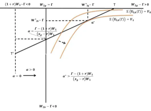
which declines as the proportion invested in the risky asset increases. However, unlike in the case with low reference levels, in this case the MRS increases as the reference level increases. In this case, an increase in already high aspirations (i.e., the reference level) will increase in the investor’s maximum willingness to pay for the risky asset as indicated by MRS. Furthermore, the MRS now depends on the loss aversion parameter and hence is part of the optimal solution. The higher the loss aversion parameter, the lower the investment in the risky asset as MRS falls with increased loss aversion.

Assuming that the investor is sufficiently loss averse, i.e. λ > max{1, 1/K

}, she will

select the proportion invested in the risky asset by making the MRS, as given by (9), equal

to

as before and arrive to the optimal solution. Thus, M RS (α

, λ, Γ) =

. Figure 4

illustrates the solution.

Figure 4: High reference level: Γ > (1 + r)W

3 Conclusion

This note was written in order to explore the role of the marginal rate of substitution on the optimal choice of risky asset holdings. The MRS shows the maximum willingness to pay to have an additional unit of wealth in the good state of nature by increasing risk taking while holding expected utility constant. We find that the maximum willingness to pay to take risk decreases, remain constant or increases with the reference level depending if the reference level is set below, equal to or above the gross return from the safe asset. The MRS depends on loss aversion inversely in all cases except when the reference level is below the gross return of the safe asset. Hence, we find that the value investors place on risky assets depends not only on economic fundamentals but also on psychological factors such as loss aversion and the self-improvement and self-enhancement motives.

The implication is that changes in investors’ motives due to psychology could drive stock markets away from economic fundamentals.

References

Barberis, N. and M. Huang 2001 “Mental accounting, loss aversion, and individual stock returns” Journal of Finance 56, 1247-1292.

6

Future empirical research could explore cognitive ability and loss averse investors’ portfolio choice (see

Christelis et al. 2010).

Barberis, N., M. Huang and T. Santos 2001 “Prospect theory and asset prices” Quarterly Journal of Economics 116, 1-53.

Barberis, N., M. Huang and R.H. Thaler 2006 “Individual preferences, monetary gambles, and stock market participation: A case for narrow framing” The American economic review 96, 1069-1090.

Berk, J.B. and J. Walden 2013 “Limited capital market participation and human capital risk” Review of Asset Pricing Studies 3 , 1-37.

Berkelaar, A.B., R. Kouwenberg and T. Post 2004 “Optimal portfolio choice under loss aversion” Review of Economics and Statistics 86, 973-987.

Bernard C. and M. Ghossoub 2010 “Static portfolio choice under cumulative prospect theory”

Mathematics and Financial Economics 2, 277-306.

Christelis, D., T. Jappelli and M. Padula 2010 “Cognitive abilities and portfolio choice”

European Economic Review 54, 18-38.

De Giorgi, E.G. 2011 “Loss aversion with multiple investment goals” Mathematics and Fi- nancial Economics 5, 203-227.

Falk A. and M. Knell 2004 “Choosing the Joneses: Endogenous goals and reference stan- dards” Scandinavian Journal of Economics 106, 417-435.

Gomes, F.J. 2005 “Portfolio choice and trading volume with loss-averse investors” Journal of Business 78, 675-706.

Haliassos, M. and C.C. Bertaut 1995 “Why do so few hold stocks?” The Economic Journal 105, 1110-1129.

He, X.D. and X.Y. Zhou 2011 “Portfolio choice under cumulative prospect theory: An analytical treatment” Management Science 57, 315-331.

Hlouskova, J. and P. Tsigaris 2012 “Capital income taxation and risk taking under prospect theory” International Tax and Public Finance 19, 554-573.

Kahneman, D. and A. Tversky 1979 “Prospect theory: An analysis of decision under risk”

Econometrica 47, 263-291.

Mehra, R. and E.C. Prescott 1985 “The equity premium: A puzzle” Journal of Monetary Economics 15 , 145-161.

van Rooij, M., A. Lusardi and R. Alessie 2011 “Financial literacy and stock market partici- pation” Journal of Financial Economics 101, 449-472.

Stiglitz, J.E. 1969 “The effects of income, wealth and capital gains taxation on risk taking”

Quarterly Journal of Economics 83, 263-283.

Thaler, R.H. 2016 “Behavioral economics: Past, present and future” American Economic Review 106, 1577-1600.

Tversky, A. and D. Kahneman 1992 “Advances in prospect theory: Cumulative representa-

tion of uncertainty” Journal of Risk and Uncertainty 5, 297-323.