The Effects of Exchange-Rate Exposures on Equity Asset Markets

(1)

IHS Economics Series Working Paper 94

January 2001

The Effects of Exchange-Rate Exposures on Equity Asset Markets

Adusei Jumah

Robert M. Kunst

(2)

Impressum Author(s):

Adusei Jumah, Robert M. Kunst Title:

The Effects of Exchange-Rate Exposures on Equity Asset Markets ISSN: Unspecified

2001 Institut für Höhere Studien - Institute for Advanced Studies (IHS) Josefstädter Straße 39, A-1080 Wien

E-Mail: o ce@ihs.ac.atﬃ Web: ww w .ihs.ac. a t

All IHS Working Papers are available online: http://irihs. ihs. ac.at/view/ihs_series/

(3)

The Effects of Exchange-Rate Exposures on Equity Asset Markets

Adusei Jumah, Robert M. Kunst

94 Reihe Ökonomie

Economics Series

(4)

94 Reihe Ökonomie Economics Series

The Effects of Exchange-Rate Exposures on Equity Asset Markets

Adusei Jumah, Robert M. Kunst January 2001

Institut für Höhere Studien (IHS), Wien

(5)

Contact:

Adusei Jumah (: +43/1/599 91-234 email: jumah@ihs.ac.at

Robert M. Kunst (: +43/1/599 91-255 email: kunst@ihs.ac.at

Founded in 1963 by two prominent Austrians living in exile – the sociologist Paul F. Lazarsfeld and the economist Oskar Morgenstern – with the financial support from the Ford Foundation, the Austrian Federal Ministry of Education and the City of Vienna, the Institute for Advanced Studies (IHS) is the first institution for postgraduate education and research in economics and the social sciences in Austria. The Economics Series presents research done at the Department of Economics and Finance and aims to share “work in progress” in a timely way before formal publication. As usual, authors bear full responsibility for the content of their contributions.

Das Institut für Höhere Studien (IHS) wurde im Jahr 1963 von zwei prominenten Exilösterreichern – dem Soziologen Paul F. Lazarsfeld und dem Ökonomen Oskar Morgenstern – mit Hilfe der Ford- Stiftung, des Österreichischen Bundesministeriums für Unterricht und der Stadt Wien gegründet und ist somit die erste nachuniversitäre Lehr- und Forschungsstätte für die Sozial- und Wirtschafts- wissenschaften in Österreich. Die Reihe Ökonomie bietet Einblick in die Forschungsarbeit der Abteilung für Ökonomie und Finanzwirtschaft und verfolgt das Ziel, abteilungsinterne Diskussionsbeiträge einer breiteren fachinternen Öffentlichkeit zugänglich zu machen. Die inhaltliche

(6)

Abstract

This paper analyzes the relationship between stock returns and exchange rate changes in international markets and examines how well exchange rate volatility explains movements in stock market returns. The model-based predictions are evaluated on several cost functions.

Results from such analysis can be used to appraise the need for hedging.

Of the three examined stock indexes, the FTSE was found to be the only robust index, while the S&P 500 and the Nikkei indexes reacted to the dollar/yen exchange rates. The dollar/yen rate also improved risk prediction for the Standard&Poor futures, while the gains in forecasting from using bivariate models remained small otherwise.

Keywords

Exchange rate futures, index futures, conditional heteroskedasticity, forecasting

JEL Classifications

C32, C53, G15

(7)

Comments

(8)

1 Introduction

Traditionally, investors with international portfolios rely on two approaches to manage their assets. The …rst assumes that the bene…ts from asset diversi…cation in international markets cannot be enhanced by hedging the exchange risk (see Akdogan 1996). Thus, investors are supposed to ignore foreign exchange risk. This argument is also supported by Hauser et al.

(1994) who show that the presence of negative correlation between changes in stock and currency prices produces decreased stock variability. The second posits all assets to be hedged completely. This stems from the fact that in an era of ‡oating exchange rates, exchange rate expectations and, hence, exchange risk premiums di¤er across countries.

Although it may be true that currencies eventually return to equilibrium, implying that returns from hedging foreign exchange exposures are slight in the long run, the …rst option has been disproved (at least in the short to medium term) by the impacts on asset prices of the recent currency crises and the fall of the Euro since its inception at the beginning of 1999. The second option can also be very expensive, as the cost of hedging certain currency risk exposures often outweighs the gain in yield.

The stock market plays an important role in the whole process of …nancial intermediation. Particularly, in most industrialized countries, the shattering e¤ect of a market crash on an economy is immense because of the reac- tion of foreign investors. Furthermore, globalization has a¤ected monetary policy by changing the channel through which interest rates a¤ect demand.

Increasingly, changing exchange rate patterns signify changing investor sen- timents. Thus, asset return volatility conceived as being induced by changes in exchange rates may imply rebalancing of risks in portfolios. A better un- derstanding as to how well exchange rate volatility explains movements in stock market indexes could be helpful in identifying structural rigidities and ine¢ciencies that discourage smooth arbitrage between di¤erent …nancial markets.

This paper analyses the relationship between stock returns and exchange rate changes in international markets and examines how well exchange rate volatility explains movements in stock market returns. The relationship can be interpreted as the measure of a stock market’s exposure to currency movements.

Some recent related studies have used regression analysis based on stock returns to estimate a …rm’s exposure to its various uncertainties (see, e.g.,

(10)

Smith et al. 1989; Oxelheim and Wihlborg 1987; and Khoo 1994).

We provide empirical evidence on the dynamic e¤ects of the dollar exchange rate (i.e., the Deutschmark-US Dollar (DM/$); the Sterling-US Dollar (£/$);

and the Yen-US Dollar (U/$)) volatility on several stock indexes (DAX, FTSE, Nikkei, and Standard & Poor 500) traded on the corresponding stock exchanges by means of multivariate GARCH models. These are, respectively, the most actively traded and quoted foreign currencies and stock indexes in the world. The model-based predictions are then evaluated on several cost functions. Results from such analysis can be used to appraise the need for hedging.

The plan of the paper is as follows. Section 2 outlines the econometric techniques and provides a description of the data. Section 3 presents and analyzes the results of the time-series model estimation. Section 4 focuses on forecasting experiments. Section 5 concludes.

2 Methodology

2.1 Bivariate ARCH models

The investigation of autoregressive conditional heteroskedasticity (ARCH) was motivated by the empirical observation of temporal clustering of volatility in …nancial time series that otherwise follow the theory-based martingale property for prices in e¢cient markets. The original ARCH model by En- gle(1982) makes a Gaussian assumption for the underlying distribution and speci…es a lag polynomial for second-order dependence:

"_t =º_tp

h_t ; h_t =c+ Xp j=1

®_j"²_t¡j ; º_t »i.i.d.N(0;1):

The GARCH model (‘general ARCH’) of Bollerslev (1986) generalizes the lag polynomial form to a rational function. The most common GARCH model is GARCH(1,1) withp= 1and one lag of h_t as a further explanatory variable added to the r.h.s. Multivariate extensions are almost exclusively restricted to this speci…cation. In the following, we use a notation similar to Gourieroux (1997). From his work, we also adopt the view that ARCH models are descriptions of the conditional-moments structure of the variables (‘weak ARCH’) and hence we will not explicitly specify distribu-

(11)

tional assumptions. This also implies that estimation by Gaussian maximum- likelihood (ML) methods is to be seen as ‘quasi–ML’.

For scalar martingale-di¤erence"t, the GARCH(1,1) model reads E("_tjFt¡1) = 0 ;

E("²_tjFt¡1) = h_t =c+®"²_t¡1+¯h_t¡1 :

The …ltrationFt is built from information sets that typically are generated by the past of the process "t and hence include the past of ht if the model is stable. Coe¢cients are subject to the admissibility restrictions c >0; ®¸ 0; ¯ ¸ 0;(®; ¯) 2 f= 0g £(0;1). The stability conditions are more involved (seeNelson, 1990), and most researchers focus on the case where ®+¯ · 1; ¯ <1, which guarantees the existence of the unconditional second moment E("²_t) if ® +¯ < 1 and includes the interesting borderline ‘IGARCH’ case withE(j"tj±) <1 for± 2(0;2) if®+¯= 1.

In principle, an extension of the GARCH(1,1) model to higher dimensions is straightforward, as all scalar coe¢cients are simply replaced by matrix coe¢cients

E("_tjFt¡1) = 0 ; E("t"⁰_tjFt¡1) = Ht

vech(Ht) = vech(C) +A~vech("t¡1"⁰_t_¡₁) +B~ vech(Ht¡1) ; (1) where we use the notation "t = ("t1; : : : ; "tn)⁰ for the vector of white-noise observations. Again, systemstability depends on the properties of thefn(n+

1)=2g £ fn(n+ 1)=2g–matrices A~ and B, though such conditions are now~ becoming increasingly complicated.

The application of such multivariate GARCH models faces two main problems. First, the joint estimation of the matrix coe¢cients quickly exhausts the degrees of freedom, particularly if the system dimensionnbecomes large.

Second, the imposition of the admissibility conditions during estimation is extremely di¢cult. Therefore, various restricted models with simpli…ed admissibility conditions have been considered in the literature, see, e.g.,Baba et al., Bollerslev (1990), orHolt and Aradhyula (1990).

Alternatively, we will focus on the case of the ARCH(1) model with B~ =0. This restriction is supported by the fact that, in tentative estimation for our data sets (unreported), the two GARCH parameters® and ¯ turned out to be poorly identi…ed even in the univariate models. In the following, we also exclusively consider the casen= 2.

(12)

We adopt a variant of the block-diagonal design of Gourieroux that allows for heteroskedasticity in conditional covariances and was suggested by Kunst and Saez (1994). Because returns show substantial serial correlation, a …rst-order MA term is added to the speci…cation for the conditional expectation. In detail, we use the MA-ARCH model

Xt = ¹+"t+£"t¡1 ;

E("t"⁰_t) = Ht ;

H_t = C+Ldiag("⁰_t_¡₁A"_t¡1;"⁰_t_¡₁B"_t¡1)L⁰ : (2) The matrixLis a triangular matrix with a unit diagonal. Imposing symmetry and de…niteness of the matrices A;B;C, the model has 16 parameters: 2 intercepts in¹, 4 entries in the2£2–matrix£, 1 o¤-diagonal entry inL, and each 3 elements in the positive de…nite matricesA;B;C. The (2,1) element of L will be denoted by ¿. It can be viewed as ‘rotating’ the two factors to the two components and hence we will also refer to it as the ‘rotation parameter’.

In order to impose de…niteness restrictions in calculation, the matrices A, B, Care re-parameterized in a Choleski form. For example, A=L⁰_AL_A, where L_A is a lower triangular matrix with a positive diagonal, i.e., L_A = (~a²₁₁,0j~a12,~a²₂₂). Hence, numerical optimization of the likelihood is conducted for technical parameters ~a₁₁;~a₁₂;~a₂₂;~b₁₁; : : :, from which estimates of the el- ementsa11; : : : can be calculated by algebraic transformations.

The system model has its ‘normal’ form when L =I and C is diagonal.

Then, covariances are 0 and the ARCH e¤ects decompose into two indepen- dent variates. Another interesting case occurs if, e.g.,B=0and the variation of volatility in both variates is explained by a single factor. The latter case and similar events of degeneration deserve special attention, as they cause non-identi…ability of some parameters and, in practice, numerical problems.

A third case of special interest is A = diag(a11;0), B = diag(0; b22). Then, conditional heteroskedasticity is fully described by squared past errors. Oth- erwise, more general quadratic forms are needed. A slight generalization of this special case occurs ifA or B are singular. If A has rank one, it can be represented as (a₁; a₂)⁰(a₁; a₂) and conditional variance in the …rst error is explained by a single lagged ‘factor’(a1"t¡1;1+a2"t¡1;2)².

If both A and B have full rank, volatility in the system is described by four di¤erent combinations of past errors. It follows that the model can be poorly identi…ed for many parameter values. We have experimented with

(13)

some general-to-speci…c backward elimination of insigni…cant parameters. In most cases, point estimates turned out very similar to those reported for the unrestricted variants. Unfortunately, t–values are usually strongly in‡ated for these pre-test estimates and can become unreliable for further inference.

2.2 Causality

The investigated AR-ARCH models involve dynamic relationships among variables that indicate causal structures in the sense of Granger causation.

The concept of Granger causality (Granger1969) was originally developed in a linear framework. Several extensions to non-linear models have been suggested.

In the original de…nition, a variable X is de…ned as causing a variable Y if the linear prediction P(YjX_¡; Y_¡; Z_¡) di¤ers from the linear prediction P(YjY_¡; Z_¡)that involves only the past of Y, denoted byY_¡, and the past of some other variables of potential relevance Z_¡, assuming that Z does not contain X. In some non-linear models, linear prediction and optimum prediction di¤er and it may well be that X does not cause Y in the linear Granger sense whereas there may be causation if the linear prediction oper- atorP(:j:)is replaced by conditional expectation E(:j:). This is a non-linear extension that was suggested by some authors, see also Granger (1988).

The most general and obvious extension would be to replace prediction and expectation by the conditional distribution. This de…nition is too general for empirical usage, hence workable de…nitions are based on conditional moment characteristics.

In the AR-ARCH model, mean prediction is linear and the linear prediction and conditional expectation operator coincide, as do linear and non- linear Granger causality in the above sense. However, variance prediction may be a¤ected by a source variable even when there is no Granger causality. A special feature of ARCH models is that all potential dynamic in‡uences of this sort are re‡ected in linear variance prediction in the sense ofComte and Lieberman (2000) who de…nelinear causality in variance by

P¡

fY ¡P(YjX_¡; Y_¡; Z_¡)g²jX_¡²; Y_¡²; Z_¡²¢

6

=P¡

fY ¡P(YjY_¡; Z_¡)g²jY_¡²; Z_¡²¢ where the conditioning set X_¡² is de…ned as the linear space containing squares and cross-products ofX_¡. Evaluation of this feature requires a comparison between two models. In contrast, multivariate AR-ARCH models

(14)

and some other non-linear models permit a direct assessment of the alterna- tive de…nition of linear second-order causality, i.e.,

P¡

fY ¡P(YjX_¡; Y_¡; Z_¡)g²jX_¡²; Y_¡²; Z_¡²¢

6

= P¡

fY ¡P(YjX_¡; Y_¡; Z_¡)g²jY_¡²; Z_¡²¢

: (3)

Here, both variances are calculated conditional on the full multivariate his- tory. Events of causality and non-causality can be read o¤ theHt matrices of the ARCH model. Comte and Lieberman (2000) show that linear causality in variance is essentially equivalent to either linear Granger causality or to linear second-order causality (or both). In the present application, second-order causality can be given a natural interpretation as the spill-over of volatility fromX to Y.

In the present paper, we are interested in investigating linear Granger causality as well as linear causality in variance. Granger causality corre- sponds to the aim of mean prediction and causality in variance to risk prediction. Estimated parametric models convey information on Granger causality and on second-order causality. Forecasting experiments admit a direct evaluation of Granger causality as well as of variance causality. The sampling variation of parameter estimates often implies an apparent contradiction between the theoretical evaluation and the prediction evaluation, as we will show in the empirical part.

2.3 Data characteristics

The …rst set of data consists of index futures for the DAX, FTSE, Nikkei, and Standard & Poor 500 index series. These series are available from November 1990 to May 2000 on a daily basis. Continuous series have been constructed o¢cially in the following form. In March, June, September, and December 3-months futures were used for contracts ending three months later. In April, July, October, and January 2-months futures are used, and in the remaining months 1-month futures are compiled.

The second set of data consists of exchange rate futures for four main currencies: the rate of US dollars per pound sterling, the rate of US dollars per German mark, and the rate of Japanese yen per US dollar. While the

…rst two rates are available on a daily basis for the whole time span that was de…ned by the availability of the index futures, i.e., November 1990 to May 2000, the yen/dollar rate is only available from the beginning of

(15)

1997. In order to obtain comparable futures series for exchange rates, where only 1-month and 3-months futures were available on a daily basis, we used 3-months exchange rate futures for the contract months of March, June, September, December. For the months preceding these months we used the 1-month exchange rate futures. For the intermediate months, we used simple arithmetic averages of the 1-month and 2-months series in order to approximate the unavailable 2-months futures variable.

3 The results

3.1 Univariate ARCH models

We estimate univariate ARCH models for the four stock futures series and report the result in Table 1. We estimate univariate ARCH models for the three exchange rate futures series and report the results in Table 2. All variables have been transformed into logarithmic di¤erences in order to obtain return series.

Note that the exchange rate futures pass the e¢cient-markets criterion, as their MA coe¢cients are insigni…cant, whereas the futures returns show signi…cant serial correlation. All series show signi…cant ARCH e¤ects. It appears that the t–values are in‡ated, due to a downward bias in variance estimates that is often observed in nonlinear time-series models. However, the importance of ARCH e¤ects is con…rmed by visual inspection of second- order correlograms (cf. Weiss, 1986). In spite of the statistical signi…cance of conditional heteroskedasticity, we note that the coe¢cients ®₁ are com- paratively small and that hence the implied data-generating processes have

…nite variance and kurtosis.

3.2 Bivariate ARCH models

As outlined in Section 2.1, the formal model with all its parameters is given as

Xt =

· ¹₁

¹2

¸

+"t +

· µ₁₁ µ₁₂ µ21 µ22

¸

"t¡1 ;

E("t"⁰_t) = Ht ; Ht =

· c11 c12

c₁₂ c₂₂

¸ +

· 1 0

¿ 1

¸

(16)

£diag ("⁰_t_¡₁

· a₁₁ a₁₂ a12 a22

¸

"t¡1;"⁰_t_¡₁

· b₁₁ b₁₂ b12 b22

¸

"t¡1)

· 1 ¿ 0 1

¸ (4); in which the matricesC,A, B are estimated in their Choleski form in order to guarantee their positive de…niteness. Estimates for the ‘model parameters’

c11; c12; c22 can be retrieved from estimates for the ‘technical parameters’ ~c11,

~

c₂₂, ~c₁₂ in a second step. Estimation in the technical parameterization is conducted by a quasi–ML algorithm that imposes normality on the errors

"t. Optimization of the likelihood function uses the BFGS algorithm of

GAUSS that also calculates numerical standard errors and t–values. Due to near-singularities of some matrices, many of these standard errors appear fragile. Hence, we refrain from calculatingt–values for the transformed model parameter estimates. Therefore, whereas we give point estimates of both model and technical parameters,t–values are shown for technical parameters only.

Table 3 gives the results for a bivariate model that contains the FTSE index returns and the sterling/dollar exchange rate. The insigni…cant value of¹2 indicates that the sterling has been on a par against the dollar in the longer run, whereas the positive¹₁represents the positive long-run return for the FTSE index. The moving-average coe¢cients matrix£contains insignif- icant values only, which supports market e¢ciency. Only the (1,2) entry is marginally signi…cant, hence there is weak evidence on Granger causal e¤ects from the exchange rate to the FTSE returns. Two ARCH factors govern the series. The …rst factor is rooted primarily in the FTSE index series, though it also contains a small weight from the exchange rate. The second factor depends on the exchange rate only. The insigni…cant rotation parameter ¿ indicates that either ARCH factor just causes the volatility in its own series and that the covariance is time-constant. In short, the amount of second- order causality from the exchange rate to the FTSE is small. Curiously, the e¤ect from the dollar/mark exchange rate is slightly stronger, as we learned from a further unreported experiment.

Table 4 gives parallel results for the DAX index and the dollar/mark exchange rate. The structure of the estimated model is similar, although now there is signi…cant Granger causality from exchange rate shocks to the DAX index, thus violating market e¢ciency in the DAX futures, in slight con‡ict with the univariate evidence. Again, the evidence on second-order causality is very small.

Tables 5 to 7 consider the Standard & Poor 500 index and all three

(17)

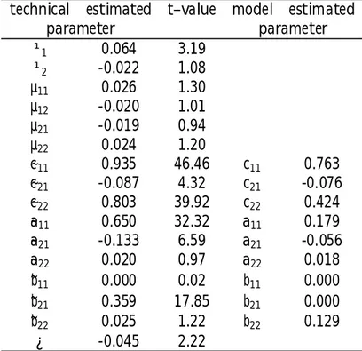
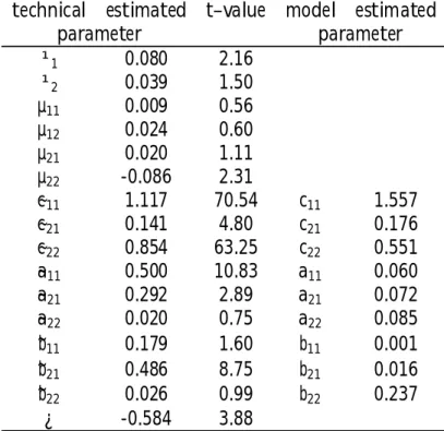
di¤erent exchange rates versus the US dollar. There appears to be little spill- over from the German mark. In contrast, the British pound and the Japanese yen are statistically signi…cant carriers of information for the S&P futures.

For both of these cases, the rotation parameter ¿ is also signi…cant, which implies that volatility in the exchange rates not only a¤ects the S&P volatility via the …rst factor but also via the second factor. For the dollar/sterling rate, the …rst factor is dominated by the S&P volatility and the parameter ¿ is still small, although statistically signi…cant. For the dollar/yen rate, the

…rst factor mixes squared shocks in both series with similar weights and the rotation parameter ¿ opens a second strong channel for the volatility spill- over. We note, however, that the dollar/yen results were obtained from a shortened time range and are therefore more likely to re‡ect the patterns of a particular episode than the other experiments. There is also strong evidence against market e¢ciency in the dollar/yen rate, which corroborates the univariate results. In the remaining cases, direct evidence on ine¢ciency remains weak, thus also enhancing the univariate models (see Tables 1 and 2).

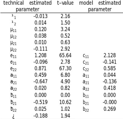
Table 8 shows that the bilateral yen/dollar exchange rate also incurs a signi…cant volatility spill-over to the Japanese Nikkei index. The Nikkei returns are signi…cantly autocorrelated and thus do not conform to market e¢ciency. The rotation parameter¿ is only marginally signi…cant. The main spill-over e¤ect to the Nikkei futures stems from the …rst ARCH factor that re‡ects a weighted average of the innovations from both series. Conditional heteroskedasticity in the covariance across both types of shocks is weaker than in the S&P experiment.

4 Forecasting experiments

As is well known, the predictive quality of an econometric model is an issue that is largely separate from other checks on its validity. Slightly misspeci…ed models can prove to be good workhorses for forecasting, whereas otherwise acceptable speci…cations can fail completely with regard to predictive accuracy. The latter feature has been often reported for models of the ARCH type (see, e.g. Jorion, 1995). It is possible that the predictive quality is of more concern to an investor than other statistical properties of the en- tertained model, hence we consider forecasting experiments to be of major relevance.

(18)

We assess the relative predictive accuracy of the reported models as follows. We estimate the univariate and bivariate models iteratively from the starting point of the available sample to a …xed end pointT0 =T¡sand then predict the next observation at time T0+ 1. We then update the parameter estimates of the models and predict the observation at time T₀+ 2. Thus, sone-step forecasts are generated that can be gauged against the known re- alizations. Because the procedure of updating the complex non-linear structures is computationally intensive, we restrict ourselves to predicting the last s= 22observations in the available sample. We note that the value ofs = 22 was chosen to represent one business month.

We consider mean predictions as well as risk predictions. Because of the speculative nature of the data and the closeness of the market structure to theoretical assumptions of e¢ciency—which were not too hardly rejected in the reported estimations—we expected that the relative results of risk predictions would be more interesting. The known di¢culty of evaluating risk predictions is that the true volatility is unknown, hence one must be satis…ed with the poor approximation of forecasting squared mean-corrected observations instead. We note that the indispensable mean correction is the main problem, as a poor forecast of the local mean may ruin a correct prediction of local volatility.

The following evaluation criteria will be used: …rstly, the mean squared error as the traditional measure of prediction accuracy; secondly, the more robust mean absolute error; thirdly, the even more robust median absolute error. The latter criterion successfully mitigates the role of local outliers that otherwise dominate the relative evaluation. All three criteria are applied to the two cases of mean and of risk prediction, hence we report six numbers for each experiment.

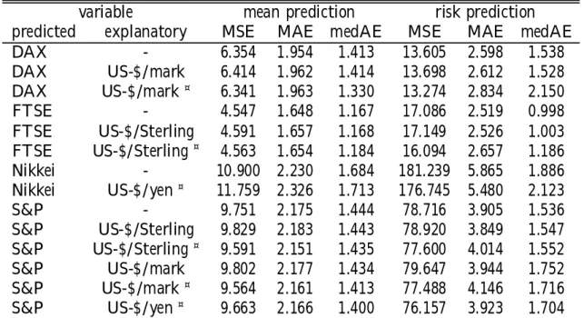
The results for index futures predictions based on univariate and bivariate ARCH models—in all cases for the stock futures indexes and not for the exchange rates—are summarized in Table 9. The comparison is disappointing.

Most of the bivariate forecasts are dominated by the corresponding univariate forecast. On the whole, the bivariate predictions appear to be slightly worse, with the noteworthy exceptions of the risk forecast for the Nikkei index and of the risk forecast for the US S&P index on the basis of the dollar/yen exchange rate. These two experiments share the common feature that they are based on a shorter sample that is dictated by the range of available yen futures. A small overall improvement relative to the univariate prediction points to the possibility that the time-series structure may have been subjected to longer-

(19)

run changes. Therefore, we re-ran all other prediction experiments basing all estimates of model parameters on the same shortened time range that was dictated by availability in the yen case. These results are marked by asterisks in Table 9. Indeed, the quality of the Standard&Poor forecasts generally in- creases for the shortened estimation range but this e¤ect is more pronounced for the mean prediction. For risk prediction, the model that uses the dollar/yen exchange rate still dominates and that based on the dollar/sterling rate even deteriorates by shortening the estimation range. This e¤ect is similar for the DAX and FTSE predictions. While mean prediction is slightly improved by shortening the estimation range, no such improvement is felt for predicting the risk.

5 Summary and conclusion

We have analyzed the relationship between stock returns and exchange rate changes in international markets and examined how well exchange rate volatility explains movements in stock market returns. The model-based predictions were evaluated on several cost functions.

Results from time-series model estimation vary considerably across countries. Whereas, in a bivariate model for the FTSE index returns and the sterling/dollar exchange rate, market e¢ciency is supported, strong evidence on violation of market e¢ciency was found for most other series. For the FTSE index and the sterling/dollar case, two ARCH factors govern the series. The rotation parameter remains insigni…cant, hence either ARCH factor just causes the volatility in its own series and the covariance is time-constant.

In short, the amount of second-order causality from the exchange rate to the FTSE is small. This also turned out to be true for the DAX index and the dollar/mark exchange rate. We also considered joint models of the Standard

& Poor 500 index and the three di¤erent exchange rates versus the US dollar. Whereas there appears to be little spill-over from the German mark, the British pound and the Japanese yen are statistically signi…cant carriers of information for the S&P futures. For both of these cases, volatility in the exchange rates a¤ects the S&P volatility via several channels. Finally, the bilateral yen/dollar exchange rate also incurs a signi…cant volatility spill-over to the Japanese Nikkei index.

With regard to the prediction experiments, we can summarize that the di¤erences in performance are too small and fragile to allow any general

(20)

recommendation. For the case of the Standard&Poor futures, it seems that only the dollar/yen rate improves risk prediction. This e¤ect cannot be explained by the shorter estimation time range that was dictated by the availability of the dollar/yen rate. For all other cases, it was found that risk prediction and mean prediction do not necessarily coincide with regard to suggesting a speci…c optimum prediction model and that signi…cant in- sample dynamic structures do not necessarily imply links that can be used systematically for forecasting.

References

[1] Akdogan, H.“A Suggested Approach to Country Selection in Interna- tional Portfolio Diversi…cation”. Journal of Portfolio Management 23, 33–39 (1996).

[2] Baba, Y., Engle, R.F., Kroner, K.F., and D. Kraft“Multivari- ate Simultaneous Generalized ARCH”. Economics Working Paper 92-5, University of Arizona, 1992

[3] Bollerslev, T.“Generalized autoregressive conditional heteroskedasticity”.Journal of Econometrics 31, 307–27 (April 1986).

[4] ________.“Modelling the Coherence in Short-Run Nominal Ex- change Rates: A Multivariate Generalized ARCH Model”. Review of Economics and Statistics 72, 498–505 (August 1990).

[5] Comte, F., and O. Lieberman“Second-order Noncausality in Multi- variate GARCH Processes”.Journal of Time Series Analysis 21, 535–58 (2000).

[6] Engle, R.F. “Autoregressive Conditional Heteroskedasticity with Es- timates of the Variance of U.K. In‡ation”. Econometrica 50, 987–1008 (1982).

[7] Gourieroux, C.ARCH Models and Financial Applications. Springer- Verlag, New York, 1997.

[8] Granger, C.W.J. “Investigating Causal Relations by Econometric Model and Cross-Spectral Methods”.Econometrica 37, 424–38 (1969).

(21)

[9] ________.“Some recent developments in a concept of causality”.

Journal of Econometrics 39, 199–211 (1988).

[10] Hauser, S., Marcus, M., and U. Yaari “Investing in Emerging Stock Markets: Is It Worthwhile Hedging Foreign Exchange Risk?”.

Journal of Portfolio Management 20, 76–81 (1994).

[11] Holt, M.T., and Aradhyula, S.V.“Price Risk in Supply Equations:

An Application of GARCH Time-Series Models to the U.S. Broiler Mar- ket”. Southern Economic Journal 57, 230–42 (1990).

[12] Jorion, P. “Predicting Volatility in the Foreign Exchange Market”.

Journal of Finance 50, 507–28 (1995).

[13] Khoo, A.“Estimation of Foreign Exchange Exposure: An Application to Mining Companies in Australia”.Journal of International Money and Finance 13, 342–63 (1994).

[14] Kunst, R.M., and Saez, M.“ARCH Structures in Cointegrated Sys- tems”. Mimeo, presented at the ISF Meeting, Stockholm, 1994.

[15] Nelson, D.F.“Stationarity and persistence in the GARCH(1,1) Mod- el”.Econometric Theory 6, 318–334 (1990).

[16] Oxelheim, L., and Wihlborg, C.-G. Macroeconomic Uncertainty:

International Risks and Opportunities for the Corporation. Wiley, Chich- ester, U.K., 1987.

[17] Smith, C.W., Smithson, C.W., and Wilford, D.S. “Managing Financial Risk”.Journal of Applied Corporate Finance 1, 27–48 (1989).

[18] Weiss, A.A. “ARMA models with ARCH errors”. Journal of Time Series Analysis 5, 129–43 (1986).

(22)

Tables and Figures

Table 1: Univariate MA–ARCH models for the stock futures series 23/11/1990-15/5/00.

parameter DAX FTSE Nikkei S&P 500

¹ 0.080 0.053 -0.005 0.064

[3.60] [3.45] [0.81] [3.61]

µ -0.038 -0.016 0.049 0.022

[1.98] [1.04] [2.80] [1.29]

®0 1.384 0.912 1.702 0.773

[58.03] [58.53] [73.57] [49.55]

® 0.176 0.174 0.161 0.189

[13.31] [12.55] [22.60] [24.53]

Note: Fitted models are of the form xt = ¹+"t +µ"t¡1 with conditional variance equationht =®0+®"²_t¡1. Figures in squared brackets aret–values.

(23)

Table 2: Univariate MA–ARCH models for the exchange rate futures series.

Time range is 23/11/1990–15/5/00, except for the Yen series with the range 1/1/1997–15/5/00.

parameter UK£ to US$ US$ to G.Mark Yen to US$

¹ 0.004 -0.019 0.017

[0.28] [1.42] [0.59]

µ 0.003 0.026 -0.103

[0.10] [1.26] [2.65]

®₀ 0.350 0.426 0.594

[57.98] [56.40] [33.03]

® 0.179 0.122 0.276

[12.08] [9.35] [10.24]

Note: see Table 1

(24)

Table 3: Bivariate model for the FTSE index and the US dollar / sterling exchange rate. Time range is 23/11/1990–15/5/2000.

technical estimated t–value model estimated

parameter parameter

¹1 0.053 2.68

¹₂ 0.005 0.39

µ11 -0.006 0.22

µ₁₂ -0.049 1.62

µ21 0.000 0.02

µ22 0.003 0.13

~

c₁₁ 0.976 109.20 c₁₁ 0.906

~

c21 0.097 6.34 c21 0.092

~

c₂₂ 0.763 114.74 c₂₂ 0.348

~

a11 0.645 23.64 a11 0.173

~

a₂₁ 0.073 1.36 a₂₁ 0.030

~

a₂₂ 0.020 0.99 a₂₂ 0.005

~b11 0.070 0.24 b11 0.000

~b21 0.425 13.42 b21 0.002

~b₂₂ 0.025 1.24 b₂₂ 0.181

¿ 0.043 1.02

Note: The (unsigned)t–values in the third column correspond to the parameters and their point estimates in the …rst and second column. In those cases where model parameters are transforms of technical parameters, these are indicated in the fourth column and point estimates are given without t–values in the …fth column.

(25)

Table 4: Bivariate model for the DAX index and the US dollar / German mark exchange rate. Time range is 23/11/1990–15/5/2000.

parameter parameter

¹1 0.081 3.42

¹₂ -0.018 1.28

µ11 -0.029 1.30

µ₁₂ 0.099 2.76

µ₂₁ -0.004 0.36

µ22 0.028 1.21

~

c₁₁ 1.085 110.12 c₁₁ 1.383

~

c21 -0.108 6.94 c21 -0.128

~

c₂₂ 0.801 113.75 c₂₂ 0.424

~

a₁₁ 0.649 24.28 a₁₁ 0.178

~

a21 0.041 0.54 a21 0.017

~

a₂₂ 0.020 1.19 a₂₂ 0.002

~b11 0.109 1.04 b11 0.000

~b₂₁ 0.361 9.47 b₂₁ 0.004

~b22 0.025 1.51 b22 0.130

¿ -0.045 1.10

Note: See Table 3.

(26)

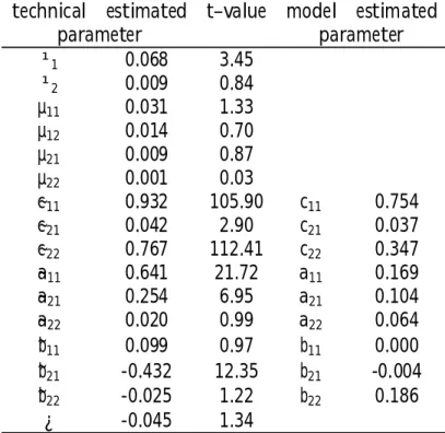
Table 5: Bivariate model for the S&P 500 index and the US dollar / German mark exchange rate. Time range is 23/11/1990–15/5/1990.

parameter parameter

¹1 0.068 3.45

¹₂ 0.009 0.84

µ11 0.031 1.33

µ₁₂ 0.014 0.70

µ₂₁ 0.009 0.87

µ22 0.001 0.03

~

c₁₁ 0.932 105.90 c₁₁ 0.754

~

c21 0.042 2.90 c21 0.037

~

c₂₂ 0.767 112.41 c₂₂ 0.347

~

a₁₁ 0.641 21.72 a₁₁ 0.169

~

a21 0.254 6.95 a21 0.104

~

a₂₂ 0.020 0.99 a₂₂ 0.064

~b11 0.099 0.97 b11 0.000

~b₂₁ -0.432 12.35 b₂₁ -0.004

~b22 -0.025 1.22 b22 0.186

¿ -0.045 1.34

Note: See Table 3.

(27)

Table 6: Bivariate model for the S&P 500 index and the US dollar / pound sterling exchange rate. Time range is 23/11/1990–15/5/2000.

parameter parameter

¹1 0.064 3.19

¹₂ -0.022 1.08

µ11 0.026 1.30

µ₁₂ -0.020 1.01

µ₂₁ -0.019 0.94

µ22 0.024 1.20

~

c₁₁ 0.935 46.46 c₁₁ 0.763

~

c21 -0.087 4.32 c21 -0.076

~

c₂₂ 0.803 39.92 c₂₂ 0.424

~

a₁₁ 0.650 32.32 a₁₁ 0.179

~

a21 -0.133 6.59 a21 -0.056

~

a₂₂ 0.020 0.97 a₂₂ 0.018

~b11 0.000 0.02 b11 0.000

~b₂₁ 0.359 17.85 b₂₁ 0.000

~b22 0.025 1.22 b22 0.129

¿ -0.045 2.22

Note: See Table 3.

(28)

Table 7: Bivariate model for the S&P 500 index and the US dollar / Japanese yen exchange rate. Time range is 1/1/1997–15/5/2000

parameter parameter

¹1 0.080 2.16

¹₂ 0.039 1.50

µ11 0.009 0.56

µ₁₂ 0.024 0.60

µ₂₁ 0.020 1.11

µ22 -0.086 2.31

~

c₁₁ 1.117 70.54 c₁₁ 1.557

~

c21 0.141 4.80 c21 0.176

~

c₂₂ 0.854 63.25 c₂₂ 0.551

~

a₁₁ 0.500 10.83 a₁₁ 0.060

~

a21 0.292 2.89 a21 0.072

~

a₂₂ 0.020 0.75 a₂₂ 0.085

~b11 0.179 1.60 b11 0.001

~b₂₁ 0.486 8.75 b₂₁ 0.016

~b22 0.026 0.99 b22 0.237

¿ -0.584 3.88

Note: See Table 3.

(29)

Table 8: Bivariate model for the Nikkei index and the US dollar / Japanese yen exchange rate. Time range is 1/1/1997–15/5/2000

parameter parameter

¹1 -0.013 2.16

¹₂ 0.014 1.50

µ11 0.120 3.24

µ₁₂ 0.038 0.52

µ₂₁ 0.010 0.63

µ22 -0.111 2.92

~

c₁₁ 1.208 65.64 c₁₁ 2.128

~

c21 -0.096 2.78 c21 -0.141

~

c₂₂ 0.871 67.30 c₂₂ 0.585

~

a₁₁ 0.459 6.80 a₁₁ 0.044

~

a21 -0.647 4.90 a21 -0.136

~

a₂₂ 0.020 0.82 a₂₂ 0.418

~b11 0.000 0.00 b11 0.000

~b₂₁ -0.519 10.62 b₂₁ -0.000

~b22 0.025 1.02 b22 0.269

¿ -0.188 1.94

Note: See Table 3.

(30)

Table 9: Prediction from univariate and bivariate ARCH models.

variable mean prediction risk prediction

predicted explanatory MSE MAE medAE MSE MAE medAE

DAX - 6.354 1.954 1.413 13.605 2.598 1.538

DAX US-$/mark 6.414 1.962 1.414 13.698 2.612 1.528

DAX US-$/mark ^¤ 6.341 1.963 1.330 13.274 2.834 2.150

FTSE - 4.547 1.648 1.167 17.086 2.519 0.998

FTSE US-$/Sterling 4.591 1.657 1.168 17.149 2.526 1.003 FTSE US-$/Sterling^¤ 4.563 1.654 1.184 16.094 2.657 1.186

Nikkei - 10.900 2.230 1.684 181.239 5.865 1.886

Nikkei US-$/yen^¤ 11.759 2.326 1.713 176.745 5.480 2.123

S&P - 9.751 2.175 1.444 78.716 3.905 1.536

S&P US-$/Sterling 9.829 2.183 1.443 78.920 3.849 1.547 S&P US-$/Sterling^¤ 9.591 2.151 1.435 77.600 4.014 1.552 S&P US-$/mark 9.802 2.177 1.434 79.647 3.944 1.752 S&P US-$/mark ^¤ 9.564 2.161 1.413 77.488 4.146 1.716 S&P US-$/yen^¤ 9.663 2.166 1.400 76.157 3.923 1.704

* estimated for the shorter time range 1997–2000.

(31)

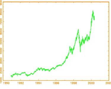
Figure 1: DAX futures series.

Figure 2: FTSE futures series.

(32)

Figure 3: Nikkei futures series.

Figure 4: Standard & Poor 500 futures series.

(33)

Figure 5: Continuous forward exchange rate pound sterling per US dollar.

Figure 6: Continuous forward exchange rate US dollars per German mark.

(34)

Figure 7: Continuous forward exchange rate Japanese yen per US dollar.