What Does it Take for a Specific Prospect Theory Type Household to Engage in Risky Investment?

IHS Economics Series Working Paper 286

April 2012

What Does it Take for a Specific Prospect Theory Type Household to Engage in Risky Investment?

Jaroslava Hlouskova

Panagiotis Tsigaris

Impressum Author(s):

Jaroslava Hlouskova, Panagiotis Tsigaris Title:

What Does it Take for a Specific Prospect Theory Type Household to Engage in Risky Investment?

ISSN: Unspecified

2012 Institut für Höhere Studien - Institute for Advanced Studies (IHS) Josefstädter Straße 39, A-1080 Wien

E-Mail: o ce@ihs.ac.atffi Web: ww w .ihs.ac. a t

All IHS Working Papers are available online: http://irihs. ihs. ac.at/view/ihs_series/

This paper is available for download without charge at:

https://irihs.ihs.ac.at/id/eprint/2131/

What Does it Take for a Specific Prospect Theory Type Household to Engage in Risky Investment?

Jaroslava Hlouskova, Panagiotis Tsigaris

286

Reihe Ökonomie

Economics Series

286 Reihe Ökonomie Economics Series

What Does it Take for a Specific Prospect Theory Type Household to Engage in Risky Investment?

Jaroslava Hlouskova, Panagiotis Tsigaris April 2012

Institut für Höhere Studien (IHS), Wien

Institute for Advanced Studies, Vienna

Contact:

Jaroslava Hlouskova

Department of Economics and Finance Institute for Advanced Studies 1060 Vienna, Austria

: +43/1/599 91-142 email: hlouskov@ihs.ac.at and Department of Economics Thompson Rivers University Kamloops, BC, Canada Panagiotis Tsigaris Department of Economics Thompson Rivers University Kamloops, BC, Canada email: ptsigaris@tru.ca

Founded in 1963 by two prominent Austrians living in exile – the sociologist Paul F. Lazarsfeld and the economist Oskar Morgenstern – with the financial support from the Ford Foundation, the Austrian Federal Ministry of Education and the City of Vienna, the Institute for Advanced Studies (IHS) is the first institution for postgraduate education and research in economics and the social sciences in Austria. The Economics Series presents research done at the Department of Economics and Finance and aims to share “work in progress” in a timely way before formal publication. As usual, authors bear full responsibility for the content of their contributions.

Das Institut für Höhere Studien (IHS) wurde im Jahr 1963 von zwei prominenten Exilösterreichern – dem Soziologen Paul F. Lazarsfeld und dem Ökonomen Oskar Morgenstern – mit Hilfe der Ford- Stiftung, des Österreichischen Bundesministeriums für Unterricht und der Stadt Wien gegründet und ist somit die erste nachuniversitäre Lehr- und Forschungsstätte für die Sozial- und Wirtschafts- wissenschaften in Österreich. Die Reihe Ökonomie bietet Einblick in die Forschungsarbeit der Abteilung für Ökonomie und Finanzwirtschaft und verfolgt das Ziel, abteilungsinterne Diskussionsbeiträge einer breiteren fachinternen Öffentlichkeit zugänglich zu machen. Die inhaltliche Verantwortung für die veröffentlichten Beiträge liegt bei den Autoren und Autorinnen.

Abstract

This research note examines the conditions which will induce a prospect theory type investor, whose reference level is set by ‘playing it safe’, to invest in a risky asset. The conditions indicate that this type of investor requires a large equity premium to invest in risky assets. However, once she does invest because of a large risk premium, she becomes aggressive and buys/sells till an externally imposed upper/lower bound is reached.

Keywords

Prospect theory, loss aversion, reference level, non-investment in risky assets

JEL Classification

D1, D8, G1

Comments

The authors acknowledge the thoughtful comments of Ines Fortin.

Contents

1 Introduction 1

2 Portfolio decisions with loss aversion 1

3 Conclusion 6

References 7

Appendix 8

1 Introduction

Although many households hold risky assets in today’s environment there is still a sizeable amount who do not own stocks (Haliassos and Bertaut, 1995). The ex- pected utility model developed by von Neumann-Morgenstern cannot provide an ad- equate explanation as to why households do not participate in the market given the large equity premium in stock markets (Mehra and Prescott, 1985; Barberis et al., 2001). Haliassos and Bertaut argue that explanations such as habit persistence, non- expected utility, market incompleteness due to uninsurable income risks and quantity constraints on borrowing are insufficient to explain this phenomenon.

Our note uses the prospect theory as developed by Kahneman and Tversky (1979) to provide an explanation for the non-investment in risky assets.

We find that a prospect theory type of investor who uses as a reference level ‘what she can earn by playing it safe’

will not invest in a risky asset as long as the expected excess return (risk premium) is within a certain threshold range. The thresholds depend on the degree of loss aversion amongst other parameters. The individual will not invest in a risky asset except if the risk premium exceeds a threshold level. Furthermore, the investor will not take a short position except if the risk premium is below another threshold level. Thus the assumption that the expected excess return is positive, as was often assumed in risk aversion expected utility models, is not a sufficient condition for the household to purchase risky investment. Finally, if the expected excess return exceeds the threshold levels then the household will engage in aggressive risky activity demanding infinite leverage to purchase or short sell the risky asset. The note proceeds as follows: In section 2 we present the basic model and investigate the main result of the paper and section 3 offers some concluding remarks.

2 Portfolio decisions with loss aversion

Consider an investor who is deciding to allocate initial wealth, W

> 0, toward a risk free investment in the amount of m and a risky investment in the amount of a. The

1See also Gomes (2005). We generalize results and incorporate the possibility of a negative expected excess return.

2I.e., comparison to an event when the household invests only in a risk free asset.

1

safe asset yields a net of the dollar investment return r > 0 and two states of nature determine the return of the risky asset, x ∈ {x

, x

}. In the good state of nature, the risky asset yields a net of the dollar investment return x

> 0 with probability p and in the bad state of nature it yields x

with probability 1 − p. Furthermore, the rates of returns of the two assets are assumed to be such that x

< r < x

.

The terminal wealth W

is determined as

W

= [(1 + r) + (x

− r)α] W

, x = x

W

= [(1 + r) + (x

− r)α] W

, x = x

)

(1) where α =

1

is the proportion of initial wealth invested in the risky asset. We assume also that the risky proportion is within the interval α

≤ α ≤ α

for final wealth to be non-negative where

α

= − 1 + r

x

− r and α

= 1 + r r − x

(2) The investor maximizes a typical Kahneman Tversky loss averse utility function given as follows

U

(W

− Γ) =

( U

(W

− Γ) =

−γ

, W

≥ Γ λU

(W

− Γ) = −λ

, 0 ≤ W

< Γ

)

where Γ is a reference wealth. The γ parameter determines the curvature of the utility function for relative gains and losses. We assume that γ ∈ (0, 1) in order to be consistent with the experimental findings of Tversky and Kahneman (1992). The λ > 1 is a loss aversion parameter which captures the fact that investors are more sensitive when they experience an infinitesimal loss in financial wealth than when experiencing a similar size relative gain. It is easy to see that in the domain W

≥ Γ the investor displays risk aversion, while in the domain of losses the investor is a risk lover. The reference wealth level is set at a level of ‘playing it safe’ when all wealth

3This can be an exogenously imposed limit on investment or short-selling. In this note we do not explore the foundations of such limits on investment.

4See Tversky and Kahneman (1992), Gomes (2005), and He and Zhou (2011) for similar utility functions.

2

is invested in the risk free asset

Γ = (1 + r)W

(3)

Thus, based on (1)-(3) the relative wealth is W

− Γ =

( (x

− r)W

α, x = x

(x

− r)W

α, x = x

and the investor solves the following problem Max

: E (U

(W

− Γ))

such that : W

− Γ = (x

− r)W

α α

≤ α ≤ α



 

 

(4)

To proceed with the analysis we define the following two thresholds Z

≡

"

λ

1 − p p

− 1

#

(1 − p)(r − x

) (5)

Z

≡

"

1 λ

1 − p

p

− 1

#

(1 − p)(r − x

) (6)

It is easy to show that Z

> Z

for λ > 1. Proposition 1 states the solution to (4).

Proposition 1 It is optimal for a prospect theory type investor not to invest in the risky asset as long as the risk premium (expected excess return) is within the interval Z

< E (x − r) < Z

.

Proof. See Appendix.

Corollary 1 The condition E (x − r) < Z

is equivalent to λ > 1/K

, where K

=

(1−p)(r−xb)^1−γ

p(xg−r)^1−γ

. On the other hand the condition E (x−r) > Z

is equivalent to λ > K

.

5Kγ showing the attractiveness of short selling the risky asset, while the inverse 1/Kγ shows the attractiveness of investing in the risky asset and coincides with the loss averse thresholds used in He and Zhou (2011).

3

Corollary 2 If E (x − r) > Z

then the investor will continue investing all of her initial wealth into the risky asset until α

= α

, while if E (x − r) < Z

then the investor will continue to short sell the risky asset until α

= α

< 0.

There are two problems to consider as shown in the Appendix. First, if α ≥ 0 the household will gain in the good state of nature and suffer losses in the bad state as in (P1) in the Appendix. Because the investor is loss averse, λ > 1, the marginal rate of substitution of increasing wealth in the good state in terms of accepting a reduction in wealth occurring in the bad state of nature, while holding utility constant, depends negatively on the loss aversion. Under (P1) the marginal rate of substitution is

d(W₂b−Γ)

d(W₂g−Γ)

|

=

−p) 1 λ

xg−r

. It is easy to show that the investor’s marginal rate of substitution will be lower than the market trade-off for wealth in the good state relative to the bad state of nature as indicated by the slope of the budget line

d(W_2b−Γ) d(W₂g−Γ)

|

=

g−r

, if E (x − r) < Z

. Hence investor will reduce the risky investment to increase utility. On the other hand, if E (x − r) > Z

then the investor will keep on increasing the investment in the risky asset until the boundary α

is reached.

Second, if α < 0 then problem (P2) applies. In a similar line of reasoning if E (x − r) > Z

then the marginal rate of substitution of wealth between good and bad state of nature,

d(W₂b−Γ)

d(W_2g−Γ)

|

=

−p)

λ

r−xb

xg−r

, is bigger than the market trade-off between wealth in the good and the bad state of nature, and the investor will reduce her short selling activity to increase utility.

Hence when preferences follow prospect theory, and the reference point is as de- scribed above, the optimal solution yields no investment in the risky asset when the risk premium is within the above boundary. The risk premium has to be above a threshold level Z

for investment in the risky asset to occur. If the risk premium is below Z

then the optimum investment is either zero or α

< 0. In order to eliminate short selling from the solution one needs to impose E (x − r) ≥ Z

instead of imposing the condition E (x − r) ≥ 0 which is required in the expected utility. Finally, if the risk premium is below Z

then short selling is attractive.

These two threshold levels, Z

and Z

depend on λ, γ, p, r and x

and could be positive or negative, but no matter what the sign is, it will always be the case that

6Gomes (2005) introduced risk aversion again in the domain of losses in order to limit the risk taking activity. We use boundaries which keep final wealth from becoming negative.

7Note thatZ²= 0 whenλ=₁

−p p

γ

which happens only forp <0.5 asλ >1.

4

Z

> Z

given λ > 1. In addition, if Z

≤ 0 then E (x − r) > 0 will be sufficient to yield a positive level of risky investment. On the other hand, a positive Z

value implies that the assumption E (x − r) > 0 will be not sufficient to cause the investor to invest in risky assets.

Furthermore as the loss averse parameter increases (decreases) the interval in which the investor will not invest in the risky asset widens (shrinks) as

> 0 and

∂Z₂

∂λ

< 0. The sensitivity of Z

and Z

to the γ parameter is not that transparent. If the investor’s loss aversion parameter is sufficiently large, i.e., λ > max n

p

1−p

,

o , then

> 0 and

< 0 and the zero optimal risky investment interval widens once again with increasing γ.

Finally, for a sufficiently loss averse prospect theory type investor (i.e., for big enough λ) Z

< 0 < Z

. For Z

to be positive the following condition is required λ >

p 1−p

. A positive Z

will definitely be met provided that the good state of nature is as likely, or less, than the probability of the bad state of nature.

The Z

threshold will be negative if λ >

1−p p

. This condition will always be met provided that the probability of the good state of nature is as probable, or more, than the bad state of nature.

With a negative Z

the investor may not engage in short selling even if she expects that the risky asset will yield less than the risk free rate E (x) < r, i.e., when Z

< E (x − r) < 0.

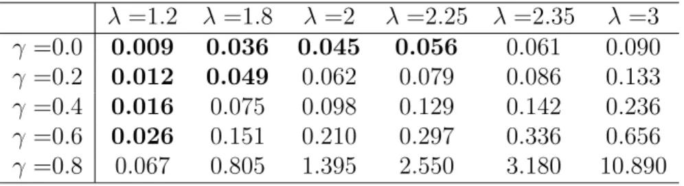
In order to illustrate this let’s consider p = 0.5, r = 2%, and assume the stock return to follow a binomial model with an expected return of 8% and a standard deviation being equal to 15%. Tables 1 and 2 show some numerical calculations of Z

and Z

by allowing λ to vary between 1.2 and 3, while γ varies between 0 and 0.8.

The bold figures in Table 1 indicate that the investor would buy the risky asset as the risk premium, E (x − r) = 6%, is above the Z

threshold. However, experiments in the literature reveal values of loss aversion in the range of 1.8 to 5 and the curvature parameter between 0.6 and 0.8 which implies that the household specified by these parameters and ‘playing it safe’ reference level would require a huge risk premium to invest in the stock market.

Had the investor’s preferences be of the expected utility

8However there are cases whenZ1<0, e.g., when 1< λ <

p 1−p

γ

andp >0.5.

9For Z² >0 it must be the case that λ <₁

−p p

γ

andp < 0.5. Namely, Z² >0 has a higher chance of occurring if the odds are in favor of a bad state of nature.

10See Abdellaoui et al. (2007) for a literature review on the estimated parameter values.

5

type then the only requirement would be a positive risk premium. On the other hand, Table 2 implies that the investor would never short sell the risky asset as the risk premium does not fall below Z

.

λ =1.2 λ =1.8 λ =2 λ =2.25 λ =2.35 λ =3 γ =0.0 0.009 0.036 0.045 0.056 0.061 0.090 γ =0.2 0.012 0.049 0.062 0.079 0.086 0.133 γ =0.4 0.016 0.075 0.098 0.129 0.142 0.236 γ =0.6 0.026 0.151 0.210 0.297 0.336 0.656 γ =0.8 0.067 0.805 1.395 2.550 3.180 10.890

Table 1: Z

threshold values given E (x − r) = 0.06 λ =1.2 λ =1.8 λ =2 λ =2.25 λ =2.35 λ =3 γ =0.0 -0.008 -0.020 -0.023 -0.025 -0.026 -0.030 γ =0.2 -0.009 -0.023 -0.026 -0.029 -0.030 -0.034 γ =0.4 -0.012 -0.028 -0.031 -0.033 -0.034 -0.038 γ =0.6 -0.016 -0.035 -0.037 -0.039 -0.040 -0.042 γ =0.8 -0.027 -0.043 -0.044 -0.044 -0.044 -0.045

Table 2: Z

threshold values given E (x − r) = 0.06

3 Conclusion

This note was written in order to explore what conditions will induce a specific prospect theory type investor whose reference level is set by ‘playing it safe’ to invest in or short sell a risky asset. Simple illustrative examples indicate that this particular investor requires a large risk premium to invest in a risky asset but once she does invest then only legal constraints can stop her investment.

However, an investor with prospect type of preferences will play the stock market if her reference level will differ from the ‘playing it safe’ level and the risk premium is positive (see Hlouskova and Tsigaris, 2012). In addition, an investor with lower degree of loss aversion will not become aggressive and thus will not engage in infinite leverage.

6

References

[1] Abdellaoui, M., H. Bleichrodt and C. Paraschiv, 2007. Loss aversion under prospect theory: A parameter-free measurement, Management Science, 53, 1659-1674.

[2] Barberis, N., M. Huang and T. Santos, 2001. Prospect theory and asset prices, Quarterly Journal of Economics, 116, 1-53.

[3] Gomes F.J., 2005. Portfolio choice and trading volume with loss-averse investors, Journal of Business, 78, 675-706.

[4] Haliassos, M. and C.C. Bertaut, 1995. Why do so few hold stocks?, The Economic Journal, 105, 1110-1129.

[5] He, X.D. and X.Y. Zhou, 2011. Portfolio choice under cumulative prospect theory: An analytical treatment, Management Science, 57, 315-331.

[6] Hlouskova, J. and P. Tsigaris, 2012. Capital income taxation and risk taking under prospect theory, International Tax and Public Finance, forthcoming.

[7] Kahneman, D. and A. Tversky, 1979. Prospect theory: An analysis of deci- sion under risk, Econometrica, 47, 263-291.

[8] Mehra, R. and E.C. Prescott, 1985. The equity premium: A puzzle, Journal of Monetary Economics, 15, 145-161.

[9] Tversky, A. and D. Kahneman, 1992. Advances in prospect theory: Cumu- lative representation of uncertainty, Journal of Risk and Uncertainty, 5, 297-323.

7

Appendix

Proof of Proposition 1. At first we re-formulate the statement of proposition 1 in more detail.

Let W

> 0, γ ∈ (0, 1), x

> −1, λ > 1, z ≡ x − r, and x

< r < x

. Then problem (4) obtains its maximum (maxima) α

as follows

(a) α

= α

for E (z) > Z

(b) α

∈ [0, α

] for E (z) = Z

(c) α

= 0 for Z

< E (z) < Z

(d) α

= α

for E (z) < Z

(e) α

∈ [α

, 0] for E (z) = Z

Note that α

≥ 0 for E (z) > Z

.

Based on the domain of α, there are two cases that can occur: 0 ≤ W

< Γ, W

≥ Γ or W

≥ Γ, 0 ≤ W

< Γ. Thus, the corresponding problems we would like to solve are

Max

: pU

(W

− Γ) + (1 − p)λU

(W

− Γ) =

(W₁α)^1−γ

1−γ

[p(x

− r)

− λ(1 − p)(r − x

)

] such that : 0 ≤ α ≤ α



 

 

(P1)

Max

: pλU

(W

− Γ) + (1 − p)U

(W

− Γ) =

(W₁(−α))^1−γ

1−γ

[−λp(x

− r)

+ (1 − p)(r − x

)

] such that : α

≤ α ≤ 0



 

 

(P2)

Case (a): Note that E (z) > Z

implies that

p(x

− r)

− λ(1 − p)(r − x

)

> 0 (A1)

8

and thus the utility function of problem (P 1) is increasing at its domain. It follows from (A1) and λ > 1 that

λp(x

− r)

− (1 − p)(r − x

)

> 0 (A2) and thus the utility function of problem (P 2) is also increasing at its domain. Based on this and the fact that utility functions of (P 1) and (P 2) are zeros for α = 0 it follows that in case (a) the utility E (U

(W

−Γ)) is increasing function in its domain and thus α

= α

.

Case (b): Note that E (z) = Z

implies that

p(x

− r)

− λ(1 − p)(r − x

)

= 0

and thus the utility function of (P 1) is constant (namely zero) in its domain. It follows from this and λ > 1 that λp(x

− r)

− (1 − p)(r − x

)

> 0 and thus the utility function of (P 2) is increasing at its domain. Thus, in case (b) the utility E (U

(W

− Γ)) has its maxima in [0, α

].

Case (c): Let Z

< E (z) < Z

. Note that E (z) < Z

implies that p(x

− r)

− λ(1 − p)(r − x

)

< 0

and thus the utility function of (P 1) is decreasing at its domain. E (z) > Z

implies (A2) and thus the utility function of (P 2) is increasing at its domain. In summary, the utility E (U

(W

− Γ)) has its maxima at zero, i.e., α

= 0.

Case (d): Note that E (z) < Z

implies that

λp(x

− r)

− (1 − p)(r − x

)

< 0

thus the utility function of (P 2) is decreasing at its domain. It follows from this and λ > 1 that p(x

− r)

− λ(1 − p)(r − x

)

< 0 and thus the utility function of (P 1) is also decreasing at its domain. The utility E (U

(W

− Γ)) is then decreasing function in its domain and reaches its maximum at α

= α

.

9

Case (e): Note that E (z) = Z

implies that

λp(x

− r)

− (1 − p)(r − x

)

= 0

and thus the utility function of (P 2) is constant (namely zero) in its domain. It follows from this and λ > 1 that p(x

− r)

− λ(1 − p)(r − x

)

< 0 which implies that the utility function of (P 1) is decreasing at its domain. Thus, in case (e) the utility E (U

(W

− Γ)) has its maxima in [α

, 0]. This concludes the proof.

10

Authors: Jaroslava Hlouskova, Panagiotis Tsigaris

Title: What Does it Take for a Specific Prospect Theory Type Household to Engage in Risky Investment?

Reihe Ökonomie / Economics Series 286 Editor: Robert M. Kunst (Econometrics)

Associate Editors: Walter Fisher (Macroeconomics), Klaus Ritzberger (Microeconomics) ISSN: 1605-7996

© 2012 by the Department of Economics and Finance, Institute for Advanced Studies (IHS),

Stumpergasse 56, A-1060 Vienna •  +43 1 59991-0 • Fax +43 1 59991-555 • http://www.ihs.ac.at

ISSN: 1605-7996