The consumption-investment decision of a prospect theory household: A two-period model with an endogenous second period reference level

IHS Economics Series Working Paper 344

November 2018

The consumption-investment decision of a prospect theory household: A two-period model with an endogenous second period reference level

Jaroslava Hlouskova

Ines Fortin

Panagiotis Tsigaris

Impressum Author(s):

Jaroslava Hlouskova, Ines Fortin, Panagiotis Tsigaris Title:

The consumption-investment decision of a prospect theory household: A two-period model with an endogenous second period reference level

ISSN: 1605-7996

2018 Institut für Höhere Studien - Institute for Advanced Studies (IHS) Josefstädter Straße 39, A-1080 Wien

E-Mail: o ce@ihs.ac.atffi Web: ww w .ihs.ac. a t

All IHS Working Papers are available online: http://irihs. ihs. ac.at/view/ihs_series/

This paper is available for download without charge at:

https://irihs.ihs.ac.at/id/eprint/4837/

The consumption-investment decision of a prospect theory household: A two-period model with an endogenous second

period reference level

Jaroslava Hlouskova

Macroeconomics and Economic Policy, Institute for Advanced Studies, Vienna, Austria Department of Economics, Thompson Rivers University, Kamloops, BC, Canada

Ines Fortin

Macroeconomics and Economic Policy, Institute for Advanced Studies, Vienna, Austria

Panagiotis Tsigaris

Department of Economics, Thompson Rivers University, Kamloops, BC, Canada

∗Jaroslava Hlouskova gratefully acknowledges financial support from the Austrian Science Fund FWF (project number V 438-N32).

Abstract

In this paper we analyze the two-period consumption-investment decision of a house- hold with prospect theory preferences and an endogenous second period reference level which captures habit persistence in consumption and in the current consumption reference level. In particular, we examine three types of household depending on how the house- hold’s current consumption reference level relates to a given threshold which is equal to the average discounted endowment income. The first type of household has a relatively low reference level (less ambitious household) and can avoid relative consumption losses in both periods. The second type of household (balanced household) always consumes exactly its reference levels. The third type of household has a relatively high reference level (more ambitious household) and cannot avoid to incur relative consumption losses, either now or in the future. Note that these households may act very differently from one another and thus there will often be a diversity of behavior. For all three types we examine how the household reacts to changes in: income (e.g., income fall caused by recession or taxation of endowment income), persistence to consumption, the first period reference level and the degree of loss aversion. Among others we find that the household increases its exposure to risky assets in good economic times if it is less ambitious and in bad economic times if it is more ambitious. We also find that in some cases more income can lead to less happiness. In addition, the less ambitious household and the more ambi- tious household with a higher time preference will be less happy with a rising persistence in consumption while the more ambitious household with a lower time preference will be happier if it sticks more to its consumption habits. Finally, the household will be happiest for the lowest possible current consumption reference level, i.e., not comparing at all will lead to the highest level of happiness.

Keywords: prospect theory, loss aversion, consumption-savings decision, portfolio allo- cation, happiness, income effects

JEL classification: G02, G11, E20

1 Introduction

One of the most important decisions households face is consumption today versus consump- tion in the future. Households transfer current consumption into the future by allocating their savings into different types of assets some of which are riskier than others. These decisions are done with the knowledge that the future is risky. The expected utility theory (EUT) has been the cornerstone model for exploring these household decisions. This research deviates from the EUT model and explores, in a two-period model, the behavior of households which are characterized by reference dependent preferences (Kahneman and Tversky, 1979; Tversky and Kahneman, 1992) and by habit persistence (Abel, 1990; Campbell and Cochrane, 1999;

Constantinides, 1990; Flavin and Nakagawa, 2008; Pagel, 2017) when deciding on consump- tion, savings, and the portfolio allocation of savings. We explore the factors that influence a household’s consumption, savings and portfolio decisions when the second period reference level is assumed to depend on first period consumption and the first period consumption refer- ence level. Households have been observed to show a habit for consumption that persists into the future, and hence a habit persistence model combined with prospect theory preferences will provide new insights on such important life cycle decisions.

By incorporating prospect theory type of preferences and habit persistence we will be able to address a number of issues on consumption and risk taking behavior that have not been explored in the literature previously. How does a household make intertemporal decisions under these two behavioral traits? Does the optimal solution depend on avoiding relative losses or not? Does the optimal choice depend on whether the household is sufficiently loss averse? Is the choice dependent on the household being less or more ambitious on targets?

How do the second period reference level, consumption, risk taking, and happiness change when the first period reference level changes? Do the responses depend on the household’s level of ambition? What impact does the habit persistence in consumption have on consumption and portfolio choice? How will a household react to sudden income changes? Do happiness, current consumption and risk taking always increase when income increases? This paper will attempt to shed some light on the above questions.

The first reference levels ever used in economic research were developed by Stone (1954) and Geary (1950). The Stone-Geary utility preferences involvereference dependent utility on subsistence levels of consumption and thus subsistence levels can be considered as a special type of reference points. Under such preferences households derive utility from consumption in excess of a subsistence level. Savings and portfolio choices with subsistence consumption have been explored by Achury et al. (2012).¹ They use a Stone-Geary expected utility model to explain the empirical observations that rich people show a higher savings rate, higher holdings

1Merton (1969, 1971) used HARA preferences to examine savings and portfolio allocations in an infinite horizon expected utility model. Achury et al. (2012) added subsistence and also habit persistence to Merton’s CRRA utility function (a subset of HARA preferences).

of risky assets as a fraction of personal wealth, and face a higher volatility in consumption.

Another model that has been used is habit persistence. This model assumes that house- holds derive satisfaction from consumption relative to a reference level which in turn depends on past consumption levels. Thus current consumption affects not only a household’s current marginal utility but also its marginal utility in the next period, which may explain why the more a household consumes today the more it will want to consume tomorrow. The macroeco- nomics and finance literature uses habit persistence models to explain many puzzles, e.g., the equity premium puzzle (Abel, 1990; Constantinides, 1990; Campbell and Cochrane, 1999), excess consumption smoothing (Lettau and Uhlig, 2000) and many business cycle patterns (Boldrin et al., 2001; Christiano et al., 2005).

Reference levels are also used to compare one’s own consumption levels to others (Falk and Knell, 2004; Hlouskova, Fortin and Tsigaris, 2017). Many households are influenced by the self-enhancement motive while others are determined by theself-improvement motive. The self-enhancement motive applies when people want to feel they are better than their peers and set their references at low levels possibly reflecting the wealth of poorer people. Others with a high reference level place importance to the self-improvement motive and compare themselves with the ones who are more successful. Hlouskova, Fortin and Tsigaris (2017) use a two-period life-cycle model with a sufficiently loss averse household to investigate the impact of these psychological traits on consumption, savings, portfolio decisions, as well as on welfare.

They find that the optimal solution depends on whether the household’s present value of the consumption reference levels is below, equal to, or above the present value of its endowment income. When reference levels are below the endowment income the authors associate this with the self-enhancement motive. Under this motive the household wants to avoid relative losses in consumption in any present or future state of nature (good or bad). Hence the degree of loss aversion does not affect optimal first period consumption and risky asset holdings.

When reference levels are equal to the endowment income this is linked to the belonging motive (i.e., the sufficiently loss averse household belonging to a similar social class). They find that the sufficiently loss averse household’s first period consumption is the exogenous reference consumption level and such households avoid playing the stock market. Finally, reference levels above the endowment income are connected with the self-improvement motive.

Households with such high reference levels cannot avoid to consume below the reference level, either now or in the future. In this case loss aversion affects consumption and risky investment negatively. The current study differs from Hlouskova, Fortin and Tsigaris (2017) in that it incorporates habit persistence into the household’s behavior.

Close to our work is also a recent paper by van Bilsen et al. (2017) who investigate optimal consumption and portfolio choice paths of a loss averse household with an endogenous reference level. The uncertainty arises from risky assets and it is assumed that the time is continuous. Mainly due to loss aversion, the household’s behavior is geared towards protecting

itself against bad states of nature to avoid or to reduce losses. Consumption choices are found to adjust slowly to financial shocks. In addition, welfare losses are found to be substantial given consumption and portfolio selections are suboptimal. Curatola (2015) also analyzes optimal consumption-savings decisions of a loss averse household with a time varying reference level in a continuous-time framework and finds that a loss averse household can consume below the reference level in bad economic times. This is done in order to invest in risky assets and increase the likelihood that in the future consumption exceeds its reference level. This behavioral approach can explain why investors increase their exposure to risky assets during financial crises. In contrast, standard habit persistence models do not allow consumption to be below the reference level. Our research complements the work by van Bilsen et al. (2017) and Curatola (2015) in that it provides additional insights: as our model is a two-period life- cycle model we can derive closed-form solutions which allow us to conduct comparative static analysis to detect why certain adjustments happen and also to conduct a welfare analysis.

In this paper, we find closed-form solutions for consumption and risk taking of a loss averse household whose endogenous second period reference level depends on current consumption (habit persistence) and on reference consumption. Households who have a relatively low first period reference level are more conservative (less ambitious), which allows them to achieve relative gains in both periods in both states of nature. Households who have a relatively high first period reference level and a low discount factor are more adventurous (more ambitious) and will thus face relative losses in the bad state of nature in the second period while they will achieve relative gains in the first period and in the good state of nature in the second pe- riod. On the other hand more ambitious households who value future consumption relatively more will have first period consumption below the reference level but will maintain future consumption in both states of nature above the endogenous second period reference level. We then conduct comparative statics and examine how these different types of households react to income changes, to changes in the first period reference level, to changes in loss aversion, and to changes in habit persistence.

The main difference with respect to Hlouskova, Fortin and Tsigaris (2017), henceforth called HFT, is that this study considers also habit persistence. An increase in the consumption habit persistence will reduce current consumption but stimulate risk taking for less ambitious households, reduce both current consumption and risk taking for more ambitious households with a high time preference, and stimulate both current consumption and risk taking for more ambitious households with a low time preference. In addition, we analyze income effects, which are closely related to the effects of income taxes. Another difference between this study and HFT is that the response of first and second period consumption of less ambitious households to a change of the first period reference level is ambiguous. Finally, unlike in HFT we also consider here a scarcity constraint on consumption, i.e., the consumption in both periods can not fall below a certain value.

Note that the household’s first period reference level may be interpreted to equal the first period consumption of a reference household, the Joneses. Thenfollowing the Joneses²means that an increase of first period consumption of the Joneses will also trigger an increase of this household’s first period consumption.³ In HFT the less ambitious household and the more ambitious household with a high time preference (low discount factor) do follow the Joneses, while the more ambitious household with a low time preference (high discount factor) does not. In this study the behavior of the more ambitious household is similar, while that of the less ambitious household may be similar or different, depending on the household’s time preference: for a lower time preference (larger discount factor) the household does follow the Joneses (like in HFT), while for a higher time preference it does not. The rest of the results are somewhat similar to HFT in terms of the impact of the exogenous parameters on the choice variables but differ in terms of magnitude.

Another interesting result that was not elaborated in HFT is the reaction of the choice variables of the household to income changes. When focusing, for instance, on risk taking then less ambitious households reduce risk taking when their income falls while more ambi- tious households increase risk taking when their income shrinks, which is consistent with the observation that investors increase their exposure to risky assets during financial crises (see Curatola, 2015). Finally, the same finding as in HFT is that the highest utility is achieved for the lowest current consumption reference level (while keeping everything else unchanged).

Thus, not comparing at all (e.g., to others) leads to the highest level of happiness.

In the next section we present the model and lay out the methodology used to find the solutions. Section 3 presents the main results with a discussion and investigates the impact of income taxation. Finally, we offer some concluding remarks.

2 The two-period consumption-investment model

2.1 Model set-up

Consider a household who decides on current and future consumption within a two-period model. In the first period it decides how to allocate a non-stochastic exogenous income, Y₁ >0, to current consumption,C₁, risk-free investment, m, and risky investment, α≥0:

Y₁ =C₁+m+α=C₁+S (1)

Savings are composed of the risk-free investment and the risky investment, i.e., S =m+α.

The net of the dollar returnr_f >0 represents the yield from the safe asset. The risky asset yields a stochastic net of the dollar returnr. We assume two states of nature, good and bad.

2See Clark et al. (2008) and Falk and Knell (2004), among others.

3This will work through the household’s first period reference level which is equal to the Joneses’ first period consumption.

The good state of nature occurs with probabilityp while the bad state of nature occurs with probability 1−p. In the good state the risky asset yields net return r_g and in the bad state it yields net returnr_b. Furthermore, it is assumed that −1< r_b < r_f < r_g, 0 < p <1, and the expected return of the risky asset is greater than the return of the safe asset, namely E(r) = p r_g + (1−p)r_b > r_f. In the second period (e.g., retirement years in a two-period life-cycle model) the household consumes

C_2s=Y₂+ (1 +r_f)m+ (1 +r_s)α

where Y₂ ≥ 0 is the non-stochastic income in the second period (e.g., government pension income) and s∈ {b, g}. Note that C2g ≥C_2b as α≥0 and rg > r_b, where C2g is the second period household’s consumption in the good state of nature andC_2bin the bad state of nature.

The household is allowed to consume the non stochastic future incomeY₂ in the first period, as long as consumption exceeds its scarcity constraint in either period (i.e.,C1≥CL≥0 and C_2s≥(1 +r_f)C_L) and savings are negative. Hence, the household can partially borrow from the risk-free asset m against its future income. The gross return from total investments is equal to (1 +r_f)m+ (1 +r_s)α, s∈ {b, g}. Based on this and (1) consumption in the second period for s∈ {b, g} is

C_2s=Y₂+ (1 +r_f)(Y₁−C₁) + (r_s−r_f)α (2) Preferences are described by the following reference based utility function

U(C₁, α) =V(C₁−C¯₁) +δ V(C₂−C¯₂) (3) C¯₁ is the first period exogenous consumption reference (or comparison) level, which can be viewed, for instance, as the first period consumption of the Joneses (a reference household to which our household compares to) or their income or, alternatively, as a fraction of this household’s income. The first two types of reference level are examples of an external reference level, which relates to, e.g., people in the same neighborhood, region or country, or people with distinct demographic features, while the third one is an example of an internal reference level, which depends on, e.g., one’s own income or one’s own past consumption, see Clark et al. (2008). ¯C₂ is the second periodendogenous reference level given such that

C¯₂ = (1 +r_f)

wC₁+ (1−w) ¯C₁

(4) wherew∈[0,1]. Note that the second period endogenous reference level depends on the first period consumption and the first period consumption reference level. The weight w shows the influence of the current consumption upon the future reference level. A higherw implies a stronger dependence between the future reference level and the current consumption level.

The weightwreflects thus the consumer’s persistence to consumption habits. The weight (1−

w), on the other hand, determines the dependence of the second period consumption reference level on the first period consumption reference level. This can be seen as a habit persistence in consumption reference levels. The two weights are negatively related to each other, i.e., an increased habit persistence on current consumption implies a lower habit persistence on the first period reference level, and vice versa. The same habit-formation reference consumption level was used also in Fuhrer (2000). The assumption on the determination of the second period reference level is the main difference between this model and the one developed and analyzed in Hlouskova, Fortin and Tsigaris (2017) where the second period reference level was exogenous.

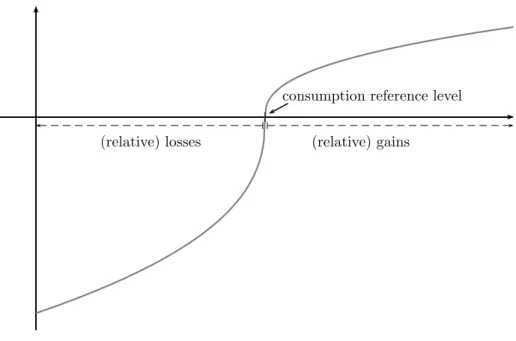
The δ is the discount factor, 0 < δ < 1, and will play an important role in the optimal solutions. A higherδ places more importance to the future relative to the presence, i.e., the household shows a lower time preference, while a smallerδ puts more weight to the presence, i.e., the household shows a higher time preference. The V(·) is a prospect theory (S-shaped) value function defined as

V(C_i−C¯_i) =











(Ci−C¯i)^1−γ

1−γ , C_i≥C¯_i

−λ^{( ¯Ci−}₁^C−ⁱγ^)1−γ, C_i<C¯_i











(5)

for i ∈ {1,2}, see Figure 1. Parameter λ > 1 represents the degree of loss aversion, while γ ∈ (0,1) represents diminishing sensitivity to consumption. Consumption in excess of the reference level represents a (relative) gain of the magnitude Ci −C¯i, while consumption below the reference level represents a(relative) loss of the magnitude equal to ¯C_i−C_i. Note that the value function is non-differentiable at the consumption reference level and is steeper in the domain of losses than in the domain of gains. This implies that there is a higher dissatisfaction from a reduction in consumption when the household is in the domain of losses than dissatisfaction from the same size of decline in consumption when the household is in the domain of gains. Finally, the household is risk averse in the domain of relative gains (i.e., the value function is concave when consumption exceeds the reference level) and risk seeking in the domain of relative losses (i.e., the value function is convex when consumption is below its reference level).

The household maximizes the following expected utility as given by (3) and (5) Max_(C1,α): E(U(C₁, α)) =V(C₁−C¯₁) +δEV(C₂−C¯₂)

such that : C₁≥C_L, C_2g ≥C_2b ≥(1 +r_f)C_L, α≥0 and C¯₂= (1 +r_f)

wC₁+ (1−w) ¯C₁

whereC_Land (1 +r_f)C_Ldetermine the minimum first and second period consumption levels,

(relative) gains (relative) losses

consumption reference level

Figure 1: Prospect theory (S-shaped) value function

so that the household does not starve (C_L ≥ 0). Based on this and (2) the household’s maximization problem can be formulated as follows

Max_(C1,α): E(U(C₁, α)) = V(C₁−C¯₁)

+ δEV (1 +r_f)(Y₁−(1−w) ¯C₁) +Y₂−(1 +r_f)(1 +w)C₁+ (r−r_f)α such that : C_L≤ C₁ ≤Y₁+_1+r^Y2

f −C_L−^r_1+r^f−rb

f α 0≤ α ≤ ^(1+rf)(Y_r^1−2CL)+Y2

f−r_b

(6) Note that the upper bound onC₁ follows fromC_2b ≥(1 +r_f)C_L and the upper bound on α follows from the imposition of the upper bound onC₁, which is at the same time larger than or equal toCL, i.e.,Y1+_1+r^Y2

f −CL−^r_1+r^f−rb

f α≥CL. Finally, the last inequality onα implies that

C_L≤ 1 2

Y₁+ Y₂ 1 +r_f

(7) which we will assume to hold. In addition we assume⁴ thatC_L≤C¯₁ and thus that

C_L≤min 1

2

Y₁+ Y₂ 1 +r_f

,C¯₁

(8)

4This is required for the feasibility of certain solutions.

2.2 Methodology

Prior to presenting the main results of the study we sketch the approach we chose to conduct the formal analysis, which requires the consideration of eight household consumption decision problems:

(P1) C¯₁ ≤C₁, C¯₂≤C_2b≤C_2g

(P2) C¯₁ ≤C₁, (1 +r_f)C_L≤C_2b ≤ C¯₂≤C_2g (P3) C¯1 ≤C1, (1 +r_f)CL≤C2g ≤ C¯2≤C_2b (P4) C¯₁ ≤C₁, (1 +r_f)C_L≤C_2b ≤C_2g≤ C¯₂

(P5) C_L≤C₁ ≤ C¯₁, C¯₂≤C_2b≤C_2g

(P6) CL≤C1 ≤ C¯1, (1 +r_f)CL≤C_2b ≤ C¯2≤C2g

(P7) C_L≤C₁ ≤ C¯₁, (1 +r_f)C_L≤C_2g ≤ C¯₂≤C_2b (P8) C_L≤C₁ ≤ C¯₁, (1 +r_f)C_L≤C_2b ≤C_2g≤ C¯₂

The first four problems (P1)–(P4) assume that the household keeps current period con- sumption equal to or above the reference level experiencing a relative gain in the first period.

In (P1) the household does not suffer from relative losses neither in the second period. In problems (P2)–(P4), however, there are relative losses: in (P2) the relative losses occur in the bad state of nature while in (P4) the relative losses are observed in both states of nature.

Note that asC_2g ≥C_2b any feasible solution for (P3) or (P7) satisfiesC_2g =C_2b = ¯C₂, which implies that any solution feasible for (P3) is feasible also for (P1), (P2) and (P4), and any solution feasible for (P7) is feasible also for (P5), (P6) and (P8). Thus, problems (P3) and (P7) can be dropped from our analysis.

In the remaining problems (P5), (P6) and (P8) current consumption is below, or equal to, its reference level and thus the household experiences relative losses in the first period.

In problem (P5) the household keeps future consumption above its reference level and suffers relative losses only in the first period. In (P6) there are losses if the bad state of nature occurs.

In the last problem (P8) there are relative losses in both periods. In what follows we show that (P1), no losses, (P2), losses in the second period in the bad state of nature, and (P5), losses only in the first period, have optimal interior solutions, and for certain conditions based on the degree of loss aversion, the size of the current reference consumption level ¯C₁, and/or the size of the discount factor one of these solutions is the solution of our main problem (6).

For higher first period consumption reference levels some of the problems have solutions at the border of the set of feasible solutions. These are problems (P4), (P6) and (P8), and their optimal solutions will not be explored in this paper.⁵

5Appendix B provides the optimal solution to all problems for a more general second period reference level C¯2 =w0+w1C1+w2C¯1, where 0≤w0 ≤(1 +rf)Y1+Y2, w1, w2 ≥0, C1 ≥C1L ≥0 and C2b ≥C2L ≥0.

To reduce the complexity in the main text we use a simpler formulation for the determination of the second period reference level, namely: w0 = 0, w1 = (1 +rf)w, w2 = (1 +rf)(1−w), w ∈ [0,1], C1L =CL ≥0

We assume that a sufficiently loss averse household makes two sequential decisions. The household first decides whether it is the less ambitious type driven by the self-enhancement motive, whether it is balanced or whether it is more ambitious governed by the self-improvement motive, and only after figuring out its level of ambition the household makes its choices for current consumption and risk taking. We treat these motives as exogenous due to the house- hold’s psychological state of mind or due to its own income or the income of the Joneses to which it compares. The less ambitious household chooses its first period consumption ref- erence level to be below some threshold level, the balanced household chooses its reference level to be equal to the threshold, and the more ambitious household chooses its first period reference consumption to be larger than the threshold. This threshold (separating less am- bitious from more ambitious households) is equal to the average (half) of the present value of total income, i.e., ¹₂

Y1+_1+r^Y2

f

. Note that the balanced household with such a neutral first period reference level will consume exactly its reference consumption in both the first and the second period.⁶ Depending on the level of ambition (and other characteristics), the sufficiently loss averse household will achieve relative gains in both periods, (P1), or current relative gains, relative gains in the good state of nature in second period but relative losses in the bad state of nature in the second period, (P2), or current relative losses and relative gains in the second period, (P5). Note finally that if the scarcity constraint exceeds the current consumption reference level (i.e.,C_L>C¯₁) then the household can achieve relative gains only in the first period⁷ and thus the optimal solution is achieved only in either (P1) or (P2).

3 Main results

In Section 3.1, we show the optimal consumption and risky asset holdings to problem (6) for aless ambitious household. The household’s solution is provided by problem (P1). The solution related to current consumption and risk taking exists for a sufficiently loss averse household with a relatively low reference level ¯C₁, namely below the threshold level, and is such that consumption exceeds the corresponding reference consumption in both periods across both states of nature. By being less ambitious the household selects consumption and risk taking in such a way as to avoid relative losses today and in the future. In addition, the household needs to be sufficiently loss averse for an optimal solution to exist in (P1), even though the loss aversion parameter does not explicitly appear in the optimal solution for current consumption and risk taking. Proposition 1 shows the closed-form solution to consumption and risk taking.

and C2L = (1 +rf)CL. Note that the model in Hlouskova, Fortin and Tsigaris (2017), which dealt with an exogenous second period consumption reference level, is imbedded in this general model, namely, when w1=w2= 0 and thus ¯C2=w0, andCL= 0.

6In this case the second period reference level will be equal to the accumulated first period reference level, i.e., ¯C2 = (1 +rf) ¯C1=¹₂[(1 +rf)Y1+Y2].

7To avoid this we assume thatCL≤C¯1, see (8).

In Section 3.2, we describe the optimal consumption and risk taking for abalanced house- hold. This is a very special situation, where the household’s first period reference level is equal to the average present value of its total wealth (neutral reference level) and hence con- sumption is exactly equal to its reference consumption in both periods. This can also be viewed as a comparison to a reference household with the same total wealth (comparison to someone like me).⁸

In Section 3.3 we show the optimal consumption and risky asset holdings to problem (6) for a more ambitious household. The solution is provided by problem (P2) or (P5). The optimal solution exists for a sufficiently loss averse household with a relatively high current reference level, namely above the threshold level, and is such that the optimal consumption is below its corresponding reference consumption in either the first or the second period.

Proposition 2 shows the closed-form solution of (6) for a more ambitious household with a high time preference (or a sufficiently large probability of the good state of nature to occur), where the solution is the solution of problem (P2), while Proposition 3 presents the closed- form solution of (6) for a more ambitious household with a low time preference, where the solution is the solution of problem (P5). In the first case the household will achieve relative gains today and in the future in the good state of nature but will incur relative losses in the future in the bad state, while in the second case the household has to accept current relative losses but will achieve relative gains in both states in the future.

As we will show, the different types of households have very distinct solutions for current consumption and risk taking activity. Also their responses, as well as the responses of the indirect utility function (happiness), to exogenous changes in the loss aversion parameter, the first period reference level, the habit persistence and finally the income/wealth levels vary substantially.

In Sections 3.4 and 3.5 we summarize the income effects and other effects across the different types of household and investigate the impact of income taxation.

3.1 Low first period reference consumption: less ambitious households In this section we consider a household with a relatively low first period reference consumption.

This reference consumption is below a certain threshold⁹ and is such that the household can consume above its reference levels in both the first and the second period, and may thus avoid any relative losses. We call a household with such a first period reference level less ambitious. This household’s behavior is captured by problem (P1). Before proceeding further,

8See Clark et al. (2008).

9Namely below the average present value of total wealth, see (11).

we introduce the following notation

Ω = (1 +r_f)Y₁+Y₂−2 (1 +r_f) ¯C₁ (9)

K_γ = (1−p)(r_f −r_b)^1−γ

p(r_g−r_f)^1−γ (10)

C¯₁^U,P1 = 1 2

Y₁+ Y₂ 1 +r_f

(11)

λ^P1−P2 =

_r

f−rb

(1+r_f)(rg−r_b+w(r_f−r_b))

1−γ

+δp h

Ω + (r_g−r_f)α^C_C^{1= ¯C1}

2b=C2L

i1−γ

δ(1−p)

(1 +r_f)( ¯C₁−C_L)1−γ

− Ω^1−γ[(1 +r_f)(1 +w) +M]^γ δ(1−p)(1 +r_f)(1 +w)

(1 +r_f)( ¯C1−CL)1−γ for ¯C₁ ≤C¯₁^P1 (12)

λ^P1−P5 =







 k2

1 +K

1

γγ

(1 +r_f)(1 +w)









γ

=

M (1 +r_f)(1 +w)

γ

(13)

k₂ =

"

δ(1 +r_f)(1 +w)p

r_g−r_b r_f −r_b

1−γ#_γ¹

(14)

M =

δ(1 +r_f)(1 +w)pr_g−r_b r_f −r_b

_γ¹

r_f −r_b+K

1 γ

0 (r_g−r_f)

r_g−r_b (15)

α^C_C^{1= ¯C1}

2b=C2L = (1 +r_f)(Y₁−C¯₁−C_L) +Y₂

r_f −r_b (16)

Note that ¯C₁ <C¯₁^U,P1is equivalent to Ω>0.¹⁰ We present the optimal solution for first period consumption and risk taking of the less ambitious household in the following proposition.

Proposition 1 Let C¯₁ <C¯₁^U,P1 and λ >max

λ^P1−P2, λ^P1−P5 . Then problem (6) obtains

10Note that HFT characterize the different types of household through Ω (being positive, equal to zero, or negative), while in this study we define the different types of household through their first period consumption reference levels (being smaller than, equal to, or larger than a threshold value), which we think makes more sense. However, we could equivalently describe our households through Ω.

a unique maximum at (C₁^∗, α^∗) = C₁^P1, α^P1

, where

C₁^P1 = C¯₁+ Ω

(1 +r_f)(1 +w) +M

= (1 +r_f)Y₁+Y₂+ [M−(1 +r_f)(1−w)] ¯C₁

(1 +r_f)(1 +w) +M >C¯₁ (17)

α^P1 =

1−K

1 γ

0

M r_f −r_b+K

1 γ

0 (rg−r_f)

C₁^P1−C¯1

>0 (18)

Proof. See Appendix B.

The future relative gains, or excess consumption, are given by:

C_2g^P1−C¯₂ = k_2r^rg−rb

f−rb C₁^P1−C¯₁

>0 C_2b^P1−C¯₂ = k₂K

1 γ

0 rg−rb

rf−rb C₁^P1−C¯₁

>0







(19)

Current relative gains, C₁^P1−C¯₁, are driving both the investment in the financial market as well as future excess consumption, see (18) and (19). The higher the relative gains in the first period the higher the investment in the financial market and the higher the relative gains (excess consumption) in the future. Note that the household invests positively in the risky asset. Total savings, however, which include both risky and risk-free assets, may be either positive or negative. The household’s consumption and risk taking does not directly depend on the degree of loss aversion; however, the household needs to be sufficiently loss averse.¹¹ Thus the optimal consumption in both periods as well as the relative consumption in both periods, risk taking and happiness are insensitive to changes in the degree of loss aversion.

The effect of an increase in the first period consumption reference level on current and future consumption cannot be determined a priori, see

dC₁^P1 dC¯₁ =

M

1+r_f −1 +w

M

1+rf + 1 +w







>0, if δ >δ¯

= 0, if δ = ¯δ

<0, if δ <δ¯

(20)

where

δ¯= 1−w 1 +K_γ^1/γ

!γ r_f −r_b r_g−r_b

1−γ 1

p(1 +w)(1 +r_f)^1−γ (21)

11As shown in Proposition 1, the loss aversion parameter needs to be sufficiently large, namely λ >

max

λ^P1−P2, λ^P1−P5 , to guarantee that the utility of (P1) at its maximum exceeds the potential maxi- mum of (P2) at its border,λ > λ^P1−P2, as well as the potential maximum of (P5) at its border,λ > λ^P1−P5. Note that problem (P1) is a concave programming problem and its unique maximum does not depend onλ.

It depends on the household’s time preference, i.e., on its discount factor, as follows: a rela- tively high discount factor (large weight placed to the future) will cause current consumption to increase with increasing ¯C₁, while a relatively low discount factor (small weight place to the future) will cause current consumption to decrease.¹² However, the effect on optimal consumption in the second period is opposite: future consumption increases with a lower dis- count factor and shrinks with a higher discount factor. In addition, the sensitivity of second period consumption in the bad state to the first period reference consumption depends on the probability of the good state. Relative current and future consumption decreases with an increasing first period reference level and also risk taking decreases when the current con- sumption reference level increases. The latter happens because the increase in the current consumption reference level decreases the relative gains in the first period discouraging in- vestment in the risky asset. Finally, an increase in the first period reference level will reduce the household’s happiness and thus the highest possible level of happiness is achieved for the lowest possible current consumption reference level. This suggests that comparison does not make oneself happy, and indeed not comparing at all would be the best. Note that the sensitivity results with respect to the first period reference level are similar (in terms of sign) to the ones when the second period consumption reference level is exogenous (see Hlouskova, Fortin and Tsigaris, 2017), except for the sensitivity of first and second period consumption: if the second period reference level is exogenous then first period consumption always increases, and second period consumption in both states of nature always decreases, with a rising first period reference level.

As stated earlier habit persistence in consumption is determined by the parameter w.

An increase in w reduces optimal first period consumption (and thus also the first period relative consumption) and the level of happiness, while it increases the investment in the risky asset. The effect of an increase inwon the second period reference level, however, is not unambiguous. It depends on the curvature,γ, the discount factor,δ, and on the level of habit persistence in consumption,w, itself. If the household is rather risk averse (γ >0.5), however, then the effect of habit persistence on the second period reference level is always positive.

Also the effect of won the second period consumption in the bad state can be either positive or negative. Namely the second period consumption in the bad state increases with increasing habit persistence in the first period consumption when w is below a certain threshold and it decreases with increasing habit persistence in the first period consumption when w exceeds the threshold.¹³ On the other hand, the impact of w on the second period consumption in the good state is always positive. Note that as habit persistence in consumption, w, relates negatively to habit persistence in the current consumption reference level, 1−w, the reported dependencies hold with the opposite sign for habit persistence in the first period reference

12Note, however, that a larger persistence in consumption reduces the threshold of the discount factor, see (21), which makes it more plausible that first period reference consumption encourages current consumption.

13This threshold is a function of the parameters describing the financial market and on the curvature.

level.

Current consumption depends positively on income, i.e., it depends positively on both first period and second period income.¹⁴ An increase in the first period income, as in good economic times, will increase current consumption by (1 +r_f)/[(1 +r_f)(1 +w) +M)], while an increase in the second period income (i.e., good future economic conditions) will increase current consumption by 1/[(1+r_f)(1+w)+M)]. Note that the presence of habit persistence in consumption has reduced the impact of income upon current consumption relative to models without such a behavioral trait. Furthermore, an increase in income will increase second period consumption as well as the relative gains (excess consumption) in both periods, the second period reference level, the investment in the risky asset and the level of happiness.

Note that a sudden reduction in income, caused by a recession or a loss of job (bad economic conditions) or by the introduction of an income tax, will cause the opposite effect and the household will thus reduce current consumption and risk taking. Note in addition that if the first period reference level is equal to a fraction of the present value of the total wealth, i.e., C¯1 = c

Y1+ _1+r^Y2

f

where c ∈ 0,¹₂

,¹⁵ then the sensitivity results will not change. This suggests that the direct income effect is stronger than the indirect effect of income through the first period consumption reference level. Table 1 summarizes the sensitivity results related to Proposition 1, which have been discussed above.

Finally, it can be shown that the expected utility evaluated at the optimal choices is determined by the relative gains in the first period:

(1−γ)E U C₁^P1, α^P1

= [(1 +r_f)(1 +w) +M]^γ

(1 +r_f)(1 +w) C₁^P1−C¯11−γ

(22) The household will be more happy with a rising income, while it will be less happy with a larger first period reference level (as the first period relative consumption decreases) and a higher persistence in current consumption, see Table 1.

C₁^∗ =C₁^P1 and α^∗ =α^P1

dC₁^∗ dC_2g^∗ dC_2b^∗ dα^∗ dC¯2 d(C₁^∗−C¯1) d(C_2g^∗ −C¯2) d(C_2b^∗ −C¯2) d(E(U(C₁^∗, α^∗)))

dλ = 0 = 0 = 0 = 0 = 0 = 0 = 0 = 0 = 0

dC¯₁ ≷0 ≶0 ≶0 <0 >0 <0 <0 <0 <0 dw <0 >0 ≶0 >0 ≶0 <0 >0 >0 <0 dY_i >0 >0 >0 >0 >0 >0 >0 >0 >0 Table 1: Sensitivity results for the less ambitious household with respect toλ, ¯C1,wand Yi, i= 1,2.

14We say that some quantity depends positively (negatively) on income, if it depends positively (negatively) on both first period income and second period income.

15The fraction needs to be less than one half such that the household is less ambitious.

3.2 Neutral first period reference consumption: balanced households This special case applies when the household is neither less ambitious (see the previous sec- tion) nor more ambitious (see the following section). The household isbalanced in the sense that it consumes exactly its reference levels, in both the first and the second period. This requires that the household’s first period reference level is equal to the threshold separating less ambitious from more ambitious households. The reference consumption is thus equal to the average of the discounted income, i.e., ¯C₁ = ¯C₁^U,P1 = ¹₂

Y₁+ _1+r^Y2

f

. We call this reference level theneutral first period reference consumption. Note that the neutral reference level depends explicitly on the household’s exogenous income. Note, in addition, that if the household’s total income coincides with the total income of some reference household then this current reference consumption can be viewed as an external reference consumption, as the household compares itself to someone like itself.

The following corollary describes the solution of the balanced household.

Corollary 1 Let C¯₁ = ¯C₁^U,P1 andλ >max

λ^P1−P2, λ^P1−P5 . Then problem (6) obtains its unique maximum at (C₁^∗, α^∗), where

C₁^∗ = 1 2

Y₁+ Y2

1 +r_f

= ¯C₁^U,P1 α^∗ = 0

Proof. See Appendix B.

The sufficiently loss averse balanced household will consume exactly its consumption ref- erence level in the first period, which is equal to half the current value of total income. In addition, it will not invest in the financial market even though the expected return from the risky asset is greater than the return from the safe asset. This phenomenon can help to explain the equity premium puzzle as it indicates that the risk premium is not sufficient to induce the household to invest in the risky asset. The savings will thus consist only of the risk-free investment, which can be positive, zero or negative, based on how the first period income and the discounted second period income relate to each other:

S=m= 1 2

Y₁− Y₂ 1 +r_f











>0 if Y₁> _1+r^Y2

f

= 0 if Y₁= _1+r^Y2

f

<0 if Y1< _1+r^Y2

f

(23)

Note, in addition, that also in the second period in both states of nature the household consumes exactly its consumption reference level, i.e., ¯C₂ =C_2g =C_2b = ¹₂[(1 +r_f)Y₁+Y₂] = (1 +r_f) ¯C₁^U,P1 = (1 +r_f) ¯C₁, which implies that this solution is feasible for all sub-problems (P1)–(P8) and thus can be considered a threshold solution, where the household achieves no relative gains and no relative losses in either period.

If the household’s income increases either in the first period and/or in the second period, while other parameters remain unchanged, including ¯C₁, then the household’s upper bound C¯₁^U,P1 will also increase and as a result the household will become relatively less ambitious since now ¯C₁<C¯₁^U,P1. Thus, the household will be able to avoid relative losses in both periods.

If on the other hand, the household’s income falls unexpectedly, while other parameters remain unchanged, then this will reduce the household’s threshold level ¯C₁^U,P1 and thus the first period reference level will be above this new upper bound ¯C₁^U,P1. As a result the household will become more ambitious in order to make up for the lost income. In this case its optimal consumption will be below the reference level either in the second period in the bad state of nature, problem (P2), or in the first period, problem (P5). We will discuss these cases in the next section.

Suppose the household has initially a current consumption reference level below the thresh- old level and hence is less ambitious. Then it is hit by a sudden reduction in income, e.g., due to a loss of job in bad economic times, which triggers a decrease of the threshold level such that the household’s (constant) reference level is above the new threshold, and hence the household is more ambitious. This switch from the less ambitious (across the balanced) to the more ambitious type will change, for example, its sensitivity of risk taking with respect to income: while before the drop in income the household (which is less ambitious) takes on less risk with decreasing income, it will be eager to take on more risk with a decreasing income – with the hope to make up for the lost income – after the drop in income (when it will be more ambitious).¹⁶

Note that consumption in both periods (as well as the relative consumption in both periods), risk taking and happiness are unaffected by changes in the level of loss aversion, as well as by changes in the persistence level in current consumption.

3.3 High first period reference consumption: more ambitious households If the first period reference level exceeds the threshold level which is equal to the average of the discounted income, i.e., if ¯C1 > C¯₁^U,P1 = ¹₂

Y1+_1+r^Y2

f

, then the household cannot consume above its reference levels in both periods. In either the first or the second period the household will have to consume below its reference consumption, and thus will incur relative losses. A household with such a high first period reference level is calledmore ambitious. The optimal consumption of the more ambitious household will be either below its consumption reference level in the second period in the bad state of nature, problem (P2), or in the first period, problem (P5). Which case occurs, problem (P2) or (P5), depends on the household’s time preference, i.e., on its discount factor, and on the probability of the good state to occur.

If the sufficiently loss averse household is relatively time impatient and assigns a low weight to future consumption (i.e., it has a small discount factor, or a high time preference) then the

16See the sensitivity results in Tables 1 and 2.

optimal solution of (6) for optimal consumption and risk taking coincides with the optimal solution of problem (P2). In this problem the optimal consumption in the first period is above its reference level, as in problem (P1). However, in the second period the household cannot avoid relative losses in the bad state of nature. Proposition 2 provides the optimal solution for this case. This case also applies if the probability of the good state of nature is sufficiently large (irrespective of the household’s time preference). On the other hand, if the discount factor is relatively large (i.e, future consumption is valued high), and the probability of the good state is not too high, then the sufficiently loss averse household will find a solution where first period consumption is below the first period reference level (suffering relative losses in the first period) but will keep future consumption above the endogenous reference level in both states of nature. The solution for this case is presented in Proposition 3. The first period reference level cannot be arbitrarily large, however. It needs to be smaller than a certain threshold, ¯C₁^U,P2.

To summarize, if the more ambitious household values first period consumption relatively high (lower discount factor), then it focuses on avoiding relative losses in the first period and thus first period consumption is above its reference level. If, however, the more ambitious household values second period consumption relatively high (larger discount factor), then it wants to prevent relative losses in the second period and consequently second period con- sumption exceeds its reference level. This is only true, however, if the probability of the good state is not too large. If it is larger than a certain threshold then only the first case applies, where relative losses occur in the second period in the bad state, irrespective of the household’s time preference.¹⁷

17Note that for better readability we will often omit the information on the large (small) enough probability of the good state of nature in identifying the type of household, and simply call a household that finds it optimal solution in problem (P2) “more ambitious with a high time preference”, and a household that finds its optimal solution in problem (P5) “more ambitious with a low time preference”.