The Consumption-Investment Decision of a Prospect Theory Household: A Two-Period Model

IHS Economics Series Working Paper 322

June 2016

The Consumption-Investment Decision of a Prospect Theory Household: A Two-Period Model

Ines Fortin

Jaroslava Hlouskova

Panagiotis Tsigaris

Impressum Author(s):

Ines Fortin, Jaroslava Hlouskova, Panagiotis Tsigaris Title:

The Consumption-Investment Decision of a Prospect Theory Household: A Two-Period Model

ISSN: 1605-7996

2016 Institut für Höhere Studien - Institute for Advanced Studies (IHS) Josefstädter Straße 39, A-1080 Wien

E-Mail: o ce@ihs.ac.at ffi Web: ww w .ihs.ac. a t

All IHS Working Papers are available online: http://irihs. ihs. ac.at/view/ihs_series/

This paper is available for download without charge at:

https://irihs.ihs.ac.at/id/eprint/3974/

The Consumption-Investment Decision of a Prospect Theory Household: A Two-Period Model ^∗

Ines Fortin

Financial Markets and Econometrics, Institute for Advanced Studies, Vienna, Austria

Jaroslava Hlouskova

Financial Markets and Econometrics, Institute for Advanced Studies, Vienna, Austria Department of Economics, Thompson Rivers University, Kamloops, BC, Canada

Panagiotis Tsigaris

Department of Economics, Thompson Rivers University, Kamloops, BC, Canada

∗

Ines Fortin and Jaroslava Hlouskova gratefully acknowledge financial support from Oesterreichische Na-

tionalbank (Anniversary Fund, Grant No. 15992).

Abstract

This study extends the literature on portfolio choice under prospect theory preferences by introducing a two-period life cycle model, where the household decides on optimal consumption and investment in a portfolio with one risk-free and one risky asset. The optimal solution depends primarily on the household’s choice of the present value of the consumption reference levels relative to the present value of its endowment income. If the present value of the consumption reference levels is set below the present value of endowment income, then the household behaves in such a way to avoid relative losses in consumption in any present or future state of nature (good or bad). As a result the degree of loss aversion does not directly affect optimal consumption and risk taking activity.

However, it must be sufficiently high in order to rule out outcomes with relative losses. On the other hand, if the present value of the consumption reference levels is set exactly equal to the present value of the endowment income, i.e., the household sets its reference levels such that they are in balance with its income, then the household’s optimal consumption is the reference consumption in both periods and the household will not invest in the risky asset. Finally, if the present value of the household’s consumption reference levels is set above the present value of its endowment income, then the household cannot avoid experiencing a relative loss in consumption, either now or in the future. As a result, loss aversion directly affects consumption and risky investment. Reference levels play a significant role in consumption and risk taking activity. In most cases the household will “follow the Joneses” if the reference levels are set equal to the consumption levels of the Joneses. Independent of how consumption reference levels are set, being more ambitious, i.e., increasing one’s reference levels, will result in less happiness. The only case when this is not true is when reference levels increase with growing income (and the present value of reference levels is set below the present value of endowment income).

Keywords: prospect theory, loss aversion, consumption-savings decision, portfolio allo- cation, happiness

JEL classification: G02, G11, E20

1 Introduction

In this paper we explore the factors that influence a household’s consumption and savings decision, based on behavioral economics preferences. Households make decisions on how much to consume today and how much to save for the future when, e.g., they retire. Savings are the means of transferring consumption into the future and of having income for retirement or the means of transferring future income to the present in order to be able to afford more consumption today. Moreover, households do not only decide how much to save but also how to allocate their savings into different types of assets. These decisions are made knowing that the future is risky and uncertain.

Traditionally, the expected utility (EUT) framework has been used to model such be- havior. ¹ This research will deviate from the EUT model and will explore a different type of preferences. In particular, we will assume prospect theory preferences that were introduced and developed by Kahneman and Tversky (1979) and Tversky and Kahneman (1992) and that take into account also psychological aspects of households’ behavior. Prospect theory can be characterized by the following properties. Decision makers under risk evaluate gains and losses with respect to some reference level, rather than evaluating absolute values (of their wealth or consumption). Households exhibit loss aversion, which means that they are more sensitive to losses than to gains of the same magnitude. In addition, households display risk aversion in the domain of gains but show risk appetite in the domain of losses, which is described by an S-shaped value function that is concave in the domain of gains and convex in the domain of losses. ² For a comprehensive overview on prospect theory see, e.g., Barberis (2013) and DellaVigna (2009).

We address a number of issues on the savings behavior under prospect theory preferences that have only partially been explored in the literature before. How do households decide on consumption and portfolio decisions when faced with prospect theory type of preferences?

Do households have to be sufficiently loss averse to yield reasonable optimal solutions for consumption and investment decisions? Does loss aversion affect consumption and portfolio decisions? Do reference levels affect the households’ consumption, savings and portfolio choice to transfer consumption into the future? If yes, how? Do households “follow the Joneses”, (i.e., compare themselves to and follow neighbors or associates) when making consumption and savings decisions?

There are many different types of reference points that can be considered in exploring the savings behavior and portfolio choice. The first reference levels that were used are subsistence levels of consumption (see, e.g., Stone, 1954 and Geary, 1951). Under such preferences, households get utility from consumption in excess of a subsistence level. Individuals have to

1

For original work in this area see Sandmo (1968, 1969) and Merton (1969, 1971).

2

Another property, not included in this study, is that the probabilities assigned to the utility of the outcomes

are not objective but subjective (so-called decision weights), as people seem to underestimate large probabilities

and overestimate small probabilities.

consume a certain minimal level irrespective of its price or the person’s income. The savings and portfolio choice with subsistence consumption has recently been explored by Achury et al. (2012). They use the Stone-Geary expected utility model to explain a number of observed empirical facts such as why the rich have a higher savings rate, higher holdings of risky assets relative to personal wealth and a higher consumption volatility than the poor.

Another commonly used reference dependent preference model is habit persistence. The habit persistence model assumes that households derive utility from consumption relative to a reference level that depends on past consumption levels. Habit persistence models have been used in many applications in macroeconomics and finance and can to some extent ex- plain, for instance, the equity premium puzzle and the behavior of asset returns (Abel, 1990;

Constantinides, 1990; Campbell and Cochrane, 1999), excess smoothness in consumption ex- penditures (Lettau and Uhlig, 2000) and business cycles characteristics (Boldrin et al., 2001;

Christiano et al., 2005).

Reference levels can also be set by comparing one’s consumption levels to others (Falk and Knell, 2004). ³ According to the psychology literature, people can be governed by self- enhancement and/or self-improvement motives. The former motive occurs when people want to make themselves feel better by setting their references at low levels, possibly reflecting the wealth of poorer people. However, people also place importance on the self-improvement motive. Here people compare themselves with others who are more successful and as a result set their reference levels high.

Many of the applications of prospect theory in portfolio selection assume that the reference level is the investor’s return from investing all initial wealth into the risk-free asset (Barberis and Huang, 2001; Gomes, 2005; Barberis and Xiong, 2009; Bernard and Ghossoub, 2010; He and Zhou, 2011). Barberis et al. (2001), Berkelaar et al. (2004), Fortin and Hlouskova (2011, 2015) and Gomes (2005) use also a dynamic updating rule for the reference point. Future utility, in one-period models, is derived from the excess return of the risky asset holdings.

One of the major findings of this literature is that investors may not invest in risky assets even if its expected return is higher than the risk-free rate.

Some work has been devoted to exploring the consequences of reference dependent pref- erences for inter-temporal two-period habit-persistence consumption decisions, when future income is uncertain and when households are loss averse, see, e.g., Bowman et al., 1999. They find that a household will resist reducing its consumption level when there is bad news about future income. Furthermore, the resistance to reducing consumption with bad news is greater than the resistance to increasing consumption in response to good news.

Koszegi and Rabin (2006) assume rational expectations in the formation of reference levels.

Assuming agents are more affected by news about current consumption than by news about future consumption, they find that people would intend to overconsume today relative to

3

For a literature review see Clark et al. (2008).

their optimal plans. They would increase consumption right away when good news regarding wealth arrives, but would postpone decreasing consumption when receiving bad news. Thus, higher wealth reduces the painful impact of bad news, and as a result people save more for precaution.

Van Bilsen et al. (2014) investigate optimal consumption and portfolio choice paths of a loss averse household but with an endogenous reference level. They find that households strive to protect themselves against consumption losses in order to avoid bad states of nature. They attribute this behavior to loss aversion. Due to the dynamic nature of their set-up they can investigate the effect of financial shocks and find that consumption choices adjust only slowly to financial shocks and that welfare losses are substantial with suboptimal consumption and portfolio selections.

Our research complements the work by Van Bilsen et al. (2014) in that it provides additional insights as discussed below. We provide a closed-form solution to the inter-temporal consumption and portfolio decision of a prospect theory household in a theoretical two-period model, where uncertainty arises from the risky asset. We assume that the asset’s return follows a Bernoulli distribution, i.e., there are two states of nature realizing with certain probabilities, and that the household’s consumption reference levels are set exogenously. These reference levels are compared with the household’s consumption levels and the household derives its utility from the difference between its consumption and the reference level. Consuming above the reference level means that the household incurs relative gains while consuming below the reference level means that it incurs relative losses. It turns out that the consumption reference levels (in both periods) as well as the loss aversion parameter are crucial in the analysis. The solution depends on the household’s choice of the consumption reference levels, more precisely, on the present value of the chosen reference levels relative to the present value of the endowment income. Hence we have three different types of households with reference levels below, equal to or above the income.

Our main results are the following. If the household sets its references levels such that

the present value is below the present value of its endowment income, then it behaves in such

a way that it avoids relative losses in any present or future state of nature (good or bad). So

optimal consumption is always above the reference level. This implies that the degree of loss

aversion does not directly affect optimal consumption and risk taking activity. However, loss

aversion must be sufficiently high in order to prevent relative losses. Further, the household

always invests in the risky asset. If, on the other hand, the household sets its references levels

such that the present value is equal to the present value of its endowment income, i.e., the

household completely balances reference levels and income, then the optimal consumption is

equal to the reference consumption in both periods. Also the household does not invest in the

risky asset in this case. Finally, if the household sets its reference levels such that the present

value is above the present value of its endowment income, then it cannot avoid relative losses

at all times. Either in the first or in the second period (good or bad state of nature) the household has to accept consuming below the reference level. This implies that loss aversion directly affects consumption and investment in the risky asset. Investment in the risky asset is again positive in this case. We look at various examples of how consumption reference levels are set, including the case when households set their reference levels according to the consumption of the “Joneses” (neighbors or associates) and examine what happens to the implied optimal consumption. Mostly prospect theory households “follow the Joneses” in the sense that their optimal consumption follows the Joneses’ consumption. Another interesting result of the sensitivity analysis is that increasing one’s reference level, i.e., increasing one’s targets and thus being more ambitious leads to less happiness. ⁴ This is true for all three types of households, i.e., independent of whether households set their consumption reference levels below, equal to, or above the income.

The paper proceeds as follows. In the next section we describe the set-up of the model. In section 3 we investigate the case where the households sets its reference levels such that the present value is below the present value of its endowment income (low aspirations). Section 4 explores the case where the present value of consumption reference levels is exactly equal to the present value of the household’s endowment income. Section 5 examines the case where the household sets its reference levels such that the present value is above the present value of its endowment income (high aspirations). Finally, we summarize and offer some concluding remarks and future extensions.

2 Problem set-up

We consider a household that lives for two periods. In the first period it receives a non- stochastic exogenous income (labor income, endowment income), Y 1 > 0, which it can allocate to current consumption, C ₁ , risk-free investment, m, and risky investment, α, where the sum of the risky and risk-free investment are savings S. Thus, in the first period

Y 1 = C 1 + m + α = C 1 + S (1)

We consider two assets, a risk-free asset with a net of the dollar return r _f > 0 and a risky asset with stochastic net of the dollar return r that yields r _g in the good state of nature, which occurs with probability p, and r _b in the bad state of nature, which occurs with probability 1 − p. We assume that −1 < r _b < r _f < r _g , 0 < p < 1, and E (r) = p r _g + (1 − p)r _b > r _f . Thus, in the second period the household consumes

C _2i = Y ₂ + (1 + r _f )m + (1 + r _i )α

4

The term “happiness” is used to denote the indirect (optimal) utility.

where Y 2 ≥ 0 is the non-stochastic income of the household in the second period, which can also be thought of as an exogenous government pension income. There are no liquidity constraints that prevent the household from consuming any exogenous future income in the first period, but consumption is not allowed to be negative in either period, so that it can only partially borrow against uncertain future income. This means that risk-free savings, m, can be negative to a certain extent. The value (1 + r _f )m + (1 + r i )α represents the wealth acquired from capital investment, i ∈ {b, g}. So, in the second period the household consumes C _2b in the bad state of nature and C _2g in the good state of nature. Based on this and (1) the consumption in the second period is

C _2i = Y ₂ + (1 + r _f )(Y ₁ − C ₁ ) + (r _i − r _f )α (2) The household’s preferences are described by the following reference based utility function

U (C ₁ , α) = V (C ₁ − C ¯ ₁ ) + δ V (C ₂ − C ¯ ₂ ) (3) where ¯ C ₁ and ¯ C ₂ are exogenous consumption reference or comparison levels, such that 0 ≤ C ¯ ₁ < Y ₁ + _1+r ^Y

²

f

and 0 ≤ C ¯ ₂ < (1 + r _f )Y ₁ + Y ₂ , i.e., Y ₁ + _1+r ^Y

²

f

> max n C ¯ ₁ , _1+r ^{C ¯}

²

f

o

, δ is the discount factor, 0 < δ < 1, and V (·) is a prospect theory (S-shaped) value function defined as

V (C _i − C ¯ _i ) =



 



 



(C

i

− C ¯

i

)

^1−γ

1−γ , C _i ≥ C ¯ _i

−λ ^{( ¯ C}

ⁱ

^−C _1−γ

ⁱ

⁾

^1−γ

, C i < C ¯ i



 



 



(4)

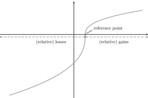
for i = 1, 2. Parameter λ > 1 is the loss aversion parameter and γ ∈ (0, 1) is the parameter determining the curvature of the utility function. If consumption is above the reference level we talk about (relative) gains, if it is below the reference level we talk about (relative) losses.

The utility has a kink at the consumption reference level and it is steeper for losses than for gains, i.e., a decrease in consumption is more severely penalized in the domain of losses than in the domain of gains. Finally, the utility function is concave above the reference point and convex below it. The household is thus risk averse in the domain of gains (i.e., above the consumption reference level) and risk seeking in the domain of losses (i.e., below the consumption reference level), see Figure 1.

The household maximizes the following expected utility as given by (3) and (4) Max _(C

₁

_,α) : E (U (C 1 , α)) = V (C 1 − C ¯ 1 ) + δ E V (C 2 − C ¯ 2 )

such that : C ₁ ≥ 0, C _2b ≥ 0, C _2g ≥ 0 and α ≥ 0

(relative) gains (relative) losses

reference point

Figure 1: Loss aversion (S-shaped) utility

Based on this and (2) the household’s maximization problem can be formulated as follows Max _(C

₁

_,α) : E (U (C ₁ , α)) = V (C ₁ − C ¯ ₁ ) + δ E V (1 + r _f )(Y ₁ − C ₁ ) + (r _i − r _f )α + Y ₂ − C ¯ ₂

such that : 0 ≤ C ₁ ≤ Y ₁ + _1+r ^Y

²

f

− ^r _1+r

^f

^−r

^b

f

α, 0 ≤ α ≤ ^(1+r _r

^f

^)Y

¹

^+Y

²

f

−r

b

(5) Note that the upper bound on C ₁ follows from C _2b ≥ 0 and the upper bound on α follows from the imposition of the upper bound on C 1 being non-negative, i.e. Y 1 + _1+r ^Y

²

f

− ^r _1+r

^f

^−r

^b

f

α ≥ 0. ⁵ The condition on α means that short sales are not allowed. ⁶

5

Imposing positive lower bounds on consumption in both periods (i.e., on C

1

, C

2b

and C

2g

), so that the household does not “starve”, would not substantially change our results. In occurrences when the optimal consumption hits zero now, it would hit the lower bound then. Thus, the behavioral implications of our findings related to the sensitivity analysis and thus comparisons to others would not change.

6

Fortin, Hlouskova and Tsigaris (2015) show that the assumption p >max n

_r

f−r_b

rg−r_b

,

^(rf−rb)

1−γ (r_f−r_b)^1−γ+(rg−r_f)^1−γ

o rules out short-selling if there is no non-negativity restriction on α. Note that E (r) > r

f

is equivalent to p >

^r_r^f−rb

g−r_b

, so only E (r) > r

f

is not sufficient to rule out short sales (except in section 3).

Before proceeding further, we introduce the following notation Ω = (1 + r _f )(Y ₁ − C ¯ ₁ ) + Y ₂ − C ¯ ₂

= (1 + r _f )

Y ₁ + Y ₂ 1 + r _f

−

C ¯ ₁ + C ¯ ₂ 1 + r _f

(6)

K γ = (1 − p)(r _f − r _b ) ^1−γ

p(r _g − r _f ) ^1−γ (7)

M =

δ(1 + r _f ) p r _g − r _b r _f − r _b

_γ¹

r _f − r _b + K

1 γ

0 (r g − r _f )

r _g − r _b (8)

In addition notice that

K 0 = (1 − p)(r _f − r _b ) p (r _g − r _f ) = K γ

r _f − r _b r _g − r _f

γ

< 1

In the following analysis we consider three fundamentally different situations, which give rise to profoundly different types of optimal consumption behavior. These situations are characterized by how the household sets its consumption reference levels in relation to its endowment income. Namely, whether the difference between the present value of total en- dowment income and the present value of the sum of the consumption reference levels is positive (Ω > 0), zero (Ω = 0), or negative (Ω < 0). ⁷ The case when Ω is positive is charac- teristic for households with low aspirations, while the case when Ω is negative is typical for households with high aspirations. The case when Ω is zero is a special case, where the present value of the household’s total endowment income is exactly equal to the present value of the consumption reference levels.

In the formal analysis we split the household’s consumption decision problem (5) into eight separate problems, (P1)–(P8), which differ in their respective domains, i.e., in their sets of feasible solutions. These domains are specified by whether first and second period (in the good and bad state of nature) consumption levels are above or below the respective reference levels. This yields a total of eight combinations, see Appendix A. Households with a positive Ω will operate on certain domains which differ from the domains on which households with a negative Ω operate.

3 Low reference values relative to endowment income (Ω > 0)

We now consider the case when the household sets its consumption reference levels such that the present value is below the present value of its endowment income, i.e., when Ω > 0. This

7

Note that Ω denotes the difference between the present value of total endowment income and the present

value of the sum of the consumption reference levels multiplied by the gross return of a dollar investment in

the risk-free rate, see equation (6). Note, in addition, that future income and consumption reference levels are

discounted at the risk-free rate.

is done when the household has low aspirations. To proceed with the analysis let us introduce the following notation

λ ^Ω≥0 = Ω ^1−γ

δ(1 − p)(1 + r _f ) ¯ C ₂ ^1−γ

"

(1 + r _f + k ₂ ) ^γ

1 + r _g − r _f r g − r _b

C ¯ ₂ Ω

1−γ

− (1 + r _f + M) ^γ

#

= 1 + r _f

k +

1 K _γ

_γ¹

! γ

Ω C ¯ 2

r g − r _b r _g − r _f + 1

1−γ

− 1 + r _f

k +

1 K _γ

_γ¹

+ 1

! γ

Ω C ¯ 2

r g − r _b r _g − r _f

1−γ

(9) We can now formulate the main result for the case when Ω > 0.

Proposition 1 Let Ω > 0 and λ > max n

1

K

γ

, λ ^Ω≥0 ,

M 1+r

f

γ o

. Then problem (5) obtains a unique maximum at (C ₁ ^∗ , α ^∗ ) where

C ₁ ^∗ = C ¯ ₁ + Ω 1 + r _f + M

= C ¯ ₁ + 1 + r _f 1 + r _f + M

Y ₁ + Y ₂ 1 + r _f

−

C ¯ ₁ + C ¯ ₂ 1 + r _f

> C ¯ ₁ (10)

α ^∗ =

1 − K

1 γ

0

M r _f − r _b + K

1 γ

0 (r _g − r _f )

(C ₁ ^∗ − C ¯ ₁ ) > 0 (11)

Proof. It follows directly from Lemma 1 in Appendix B.

When Ω is positive then aspirations are low, which should make it easier for a household to reach and exceed its consumption comparison levels than when aspirations are high. If, in addition, the utility is such that consumption below the reference levels is sufficiently penal- ized, i.e., the loss aversion parameter is large enough, then we expect optimal consumption to exceed its reference levels. This is indeed what we observe: optimal consumption levels in both periods are strictly larger than their corresponding reference levels provided that the household is sufficiently loss averse, i.e., C ₁ ^∗ > C ¯ ₁ and C _2g ^∗ ≥ C _2b ^∗ > C ¯ ₂ , where

C _2g ^∗ = C ¯ ₂ + MΩ (1 + r _f + M )

1 + K

1

γ

γ

r _g − r _b

r _f − r _b (12)

C _2b ^∗ = C ¯ ₂ + MΩ (1 + r _f + M )

1 + K

1

γ

γ

r _g − r _b r _f − r _b K

1 γ

0 (13)

Thus the optimal behavior is characterized by avoiding any relative losses to happen or, in

other words, the household’s aspirations are fully attained. We note further that optimal

investment in the risky asset is strictly positive, i.e., α ^∗ > 0, which implies that the house-

hold takes on risk in the financial market. Total savings, however, can be either positive or

negative. ⁸

Although the existence of the solution does depend on the loss aversion parameter λ, the solution itself, (C ₁ ^∗ , α ^∗ ), does not directly depend on it. The reason for this is that the household’s optimal solution is reached in problem (P1), where the solution is found in the domain given by C ₁ ≥ C ¯ ₁ , C _2b ≥ C ¯ ₂ and C _2g ≥ C ¯ ₂ , i.e., both periods’ consumption levels are above their consumption reference levels and thus the utility does not depend on the loss aversion parameter λ (see Appendix A). However, for this to happen the household needs to be sufficiently loss averse, namely λ > max n

1

K

γ

, λ ^Ω≥0 ,

M 1+r

f

γ o

. Hence, if the household is sufficiently loss averse it will make choices that avoid any relative losses from occurring.

As the domains of all remaining problems (P2)–(P8) contain a relative loss, see Appendix A, a sufficiently loss averse household will never select solutions from these problems. This behavior is only possible, however, when the household does not set its goals (consumption reference levels) too high with respect to its income, thus, when Ω is positive. ⁹ Note, finally, that problem (P1) is known from the studies on habit formation, where the consumption habits are addictive and never fall below certain consumption targets (see, for example, Yu, 2015).

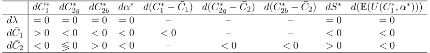
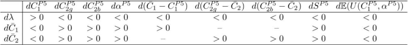
Table 1 summarizes the sensitivity results related to the solution presented in Proposition 1, so for a sufficiently loss averse household with low aspirations. In particular, we present the changes of the first and second period optimal consumption, of the optimal investment in the risky asset, of the first and second period consumption gap, of optimal savings ¹⁰ and of happiness (first row) with respect to changes in the loss aversion parameter and the first and second period consumption reference levels (first column). By “consumption gap” we mean the distance between the optimal consumption and its reference level, |C _i ^∗ − C ¯ _i |, i = 1, 2, and we use “happiness” to denote the household’s indirect utility (i.e., its value at the optimum).

We also use “relative consumption” to denote the difference between optimal consumption and the reference level, which is closely related to the previously defined consumption gap.

The gap is always positive while relative consumption can be either positive or negative. Both definitions coincide if optimal consumption is above the reference level.

Since the solution does not explicitly depend on the loss aversion parameter, as discussed above, an exogenous increase in the loss aversion parameter, keeping everything else constant, does not change the solution or the utility at the solution (happiness).

An exogenous increase in the first period consumption reference level, keeping everything else constant, will increase the first period optimal consumption, decrease risky asset hold- ings and also decrease savings. As less income is transferred to the second period we would

8

The assumption required for S

^∗

> 0 is M (Y

1

− C ¯

1

) > (Y

2

− C ¯

2

). This breaks down to simpler formulations in special cases.

9

When Ω is negative, the household cannot totally avoid relative losses. It will have to face relative losses in the first or second period, or in the good or bad state of nature.

10

The results for optimal savings follow from

^dC_dC¯^1∗

1

and Y

1

= C

₁^∗

+ S

^∗

.

dC ₁ ^∗ dC _2g ^∗ dC _2b ^∗ dα ^∗ d(C ₁ ^∗ − C ¯ ₁ ) d(C _2g ^∗ − C ¯ ₂ ) d(C _2b ^∗ − C ¯ ₂ ) dS ^∗ d( E (U (C ₁ ^∗ , α ^∗ )))

dλ = 0 = 0 = 0 = 0 – – – = 0 = 0

d C ¯ ₁ > 0 < 0 < 0 < 0 < 0 – – < 0 < 0 d C ¯ ₂ < 0 ≶ 0 > 0 < 0 – < 0 < 0 > 0 < 0

Table 1: Sensitivity results when aspirations are low (Ω > 0)

expect consumption to decrease in the second period. This is what we indeed observe: the second period consumption in either state of nature will fall with an increase in the first period consumption reference level. Even though optimal first period consumption increases in response to an exogenous increase in the first period consumption reference level, rela- tive optimal consumption in the first period, i.e., the amount by which the reference level is exceeded, decreases. This means that the extent of the increase in the first period consump- tion reference level is not fully matched by the resulting increase in the first period optimal consumption. In summary, if the household increases the first period consumption reference level it will reduce the growth rate of consumption. Finally, an increase of the first period consumption reference level decreases the happiness level.

An increase in the second period consumption reference level, keeping everything else constant, will decrease the first period optimal consumption and risky asset holdings but increase both total savings and the risk-free investment. However, the increase of the risk- free investment is not sufficient to offset the reduction in risky assets in such a way that second period consumption will increase in both states of nature. Only in the bad state of nature optimal consumption in the second period will increase. In the good state of nature the response can be either an increase or a decrease of consumption. Probably the reduced risky investment – and hence the reduced potential to achieve high returns – is the reason why this is the case. Relative optimal consumption in the second period decreases if the second period consumption reference level is increased, which is in analogy to the situation when the first period consumption level is increased. The happiness level is negatively related to the second period consumption reference level, as it was to the first period consumption reference level. So if a household is “more ambitious” (i.e., if it increases its consumption reference level), in either the first or the second period, its happiness level will decrease.

The fact that consumption reference levels are exogenous gives us the opportunity to

present some interesting examples. Consider, for instance, the case when the first period

reference level is equal to the first period consumption level of other people that the household

is associated with, i.e., the household compares itself to neighbors or peers. Then, if the

first period consumption level of the other people increases, this household will respond by

increasing its first period reference consumption level and because of this it will increase its

first period optimal consumption level, reduce risk taking and reduce its future consumption

in both states of nature. Hence, the household’s behavior is one that “follows the Joneses”

(i.e., the neighbors or peers the household wants to compare itself to). ¹¹ In addition, the gap between the household’s first period consumption and its consumption reference level narrows as the consumption level of the others increases. On the other hand, let the household’s second period reference level be equal to the expected second period consumption level of other associates. Then, if the household expects the other people to have a higher expected future consumption, it will increase its second period consumption reference level, which will reduce its first period consumption, reduce risk taking but increase risk-free investment leading to an increase in consumption in the second period in the bad state of nature but not necessarily in the good state of nature. Here it is not clear that the household follows the Joneses in the second period, even when its first period consumption is reduced to achieve an increase in future consumption like the household’s associates. However, the consumption gap in the second period declines in both states of nature when the second period consumption reference increases, bringing closer to the reference the consumption levels in the second period.

In what follows we will refer to “following the Joneses” in the first period when the increase (or decrease) of the first period consumption of the Joneses (a reference household) impacts this household such that its first period consumption will change in the same way as the one of the Joneses. I.e., it will increase, if the first period consumption of the Joneses increased and decrease if the first period consumption of the Joneses decreased. In our set-up this works in the way that the household adjusts its consumption reference level according to what the Joneses do. So it will increase its first period consumption reference level if the Joneses increase their first period consumption. In addition, we will refer to the “following the Joneses” in the second period when the increase (or decrease) of the expected second period consumption of the Joneses impacts the second period expected consumption (of the household under considerations) such that it will change in the same way as that of the Joneses. As before, the household will increase its second period consumption reference level if the Joneses increase their second period expected consumption. So the idea of “following the Joneses” is to introduce external preferences into the household’s behavior. Based on this terminology we can say that a sufficiently loss averse household with low aspirations follows the Joneses in the first period but not necessarily in the second period.

If a household sets its reference levels according to the consumption of richer peers (the rich Joneses) who consume at higher levels and wants to catch up by increasing its reference levels, then this will decrease its happiness. If, on the other hand, a household compares itself to poorer peers (the poor Joneses) that consume at lower levels and wants to adapt to the others by decreasing its reference levels, then this will increase its happiness. So comparing yourself to richer people makes you less happy while comparing yourself to poorer people makes you happier.

11

See Clark, Frijters and Shields, (2008).

Some examples of reference consumption levels for Ω > 0

In the following we present some additional interesting examples of reference consumption levels ¯ C ₁ and ¯ C ₂ .

Example 1 (Merton type expected utility): C ¯ ₁ = ¯ C ₂ = 0

A special case embedded in this behavioral study is the traditional expected utility (EUT), where ¯ C ₁ = ¯ C ₂ = 0 and thus V (C _i ) ≡ ^C _1−γ

^i1−γ

for C ₁ , C ₂ ≥ 0. In this case we solve problem (P1) and the solution is then identical to (10) and (11) for the prospect theory utility with C ¯ 1 = ¯ C 2 = 0. Thus, the optimal consumption in the first period is

(C ₁ ^∗ ) ^{EU T} = 1 + r _f 1 + r _f + M

Y ₁ + Y ₂ 1 + r _f

> 0

Note that in this case Ω ^{EU T} > Ω > 0, where Ω is related to a prospect theory (PT) household and we assume that the PT household has at least one consumption reference level strictly positive, i.e., either ¯ C ₁ > 0 or ¯ C ₂ > 0, otherwise it boils down to the expected utility case.

EUT optimal consumption is proportional to the present value of endowment income, where the factor of proportionality, representing the marginal propensity to consume out of the present value of total income, is less than unity. This marginal propensity to consume (out of the present value of total income) is the same as the one under PT preferences, assuming the curvature parameter γ remains unchanged.

In addition,

(α ^∗ ) ^{EU T} =

1 − K

1 γ

0

M r _f − r _b + K

1 γ

0 (r g − r _f )

(C ₁ ^∗ ) ^{EU T} > 0

and thus the household’s investment in the risky asset is also proportional to the present value of endowment income. ¹² However, the EUT household will always invest in the risky asset, which is not necessarily the case for the PT household when Ω = 0 and thus it will not invest in the risky financial market. The case when Ω = 0 is discussed in section 4. Note that for the EUT household the savings, (S ^∗ ) ^{EU T} = Y ₁ − (C ₁ ^∗ ) ^{EU T} , are positive when M Y ₁ > Y ₂ , in which case the household transfers some of its first period income into the second period.

Example 2 (comparison to poorer peers): C ¯ ₁ + _1+r ^{C ¯}

²

f

= Y ₁ ^P + _1+r ^Y

^2P

f

< Y ₁ + _1+r ^Y

²

f

12

In comparing optimal consumption and risky asset holdings between the two models one has to be careful

and remember that the types of utility functions suggested by these models are different. For example, the EUT

model implies a constant relative risk aversion, which is equal to γ, while the PT utility shows a decreasing

relative risk aversion, which is equal to γC

1

/(C

1

− C ¯

1

) for C

1

6= ¯ C

1

and γC

2

/(C

2

− C ¯

2

) for C

2

6= ¯ C

2

. In

addition, the relative risk aversion for the EUT model is restricted to be below one (as a consequence from

our restriction on γ, which states 0 < γ < 1), while it has sometimes empirically been found to be larger than

one (see Ahsan and Tsigaris, 2009, who provide some empirical examples).

In this situation the household with income levels Y 1 and Y 2 sets its first and second period consumption reference levels such that its present value of total reference consumption is equal to the present value of the endowment income stream of some poorer household. By a poorer household we mean a household whose total discounted endowment income is below the total discounted endowment income of this household. Namely, Y ₁ ^P + _1+r ^Y

^2P

f

< Y ₁ + _1+r ^Y

²

f

, where Y ₁ ^P and Y ₂ ^P are the first and the second period income levels of the poorer household such that Y ₁ ^P ≥ 0 and Y ₂ ^P ≥ 0. In this case Ω represents the household’s wealth net of the wealth of the poorer household, i.e., Ω = (1 + r _f ) h

Y ₁ + _1+r ^Y

²

f

−

Y ₁ ^P + _1+r ^Y

^2P

f

i

> 0. In other words, less ambitious households place themselves into the comfort zone by comparing themselves to peers with a smaller wealth level. The impact of changes in the poorer household’s income on this household’s consumption and investment behavior were discussed previously as examples of changes in the reference levels. Note that the EUT model, example 1, is observationally equivalent to households who compare themselves to people that have no endowment income, i.e., Y ₁ ^P = Y ₂ ^P = 0.

Example 3 (consumption overreaction to income): C ¯ 1 = ¯ C +cY 1 , C ¯ 2 = (1 + r _f ) ¯ C +cY 2

where ¯ C ∈ h

−c min n Y ₁ , _1+r ^Y

²

f

o , ^1−c ₂

Y ₁ + _1+r ^Y

²

f

and c ∈ (0, 1)

In this case, the consumption reference levels are set such that one part, ¯ C or (1 + r _f ) ¯ C, is independent of the household’s current income and the remaining part is a fraction of its respective income. ¹³ In order to satisfy the Ω = (1 − c) ((1 + r _f ) Y ₁ + Y ₂ ) − 2(1 + r _f ) ¯ C > 0 assumption we require ¯ C < ^1−c ₂

Y ₁ + _1+r ^Y

²

f

. In addition we assume ¯ C ≥ −cY ₁ such that C ¯ ₁ ≥ 0 and we assume ¯ C ≥ − _1+r ^c

f

Y ₂ such that ¯ C ₂ ≥ 0. In this model the household increases reference consumption levels if its endowment income increases, so aspirations increase with growing income. The optimal first period consumption and investment in the risky asset are

C ₁ ^∗ = M − (1 + r _f )

1 + r _f + M C ¯ + 1 + r _f + cM

1 + r _f + M Y 1 + 1 − c

1 + r _f + M Y 2 > C ¯ 1 , α ^∗ =

1 − K

1 γ

0

M r _f − r _b + K

1 γ

0 (r _g − r _f )

(C ₁ ^∗ − C ¯ ₁ ) > 0

Note that now an increase in the first period income has a larger effect on optimal consumption than in the case when the first period reference level is independent of income. The reason why marginal propensity to consume is larger is that two effects are operating. First, the household increases consumption because of the increase in income and second, this effect is reinforced with an increase in the first period reference level. This situation can thus be seen as a consumption overreaction to current income changes. Note, in addition, that the

13

All the statements made for example 3 would not change qualitatively if one used the same exogenous

part of the reference level in both periods ( ¯ C

1

= ¯ C + cY

1

, C ¯

2

= ¯ C + cY

2

), different fractions of income in the

two periods ( ¯ C

1

= ¯ C + c

1

Y

1

, C ¯

2

= (1 + r

f

) ¯ C + c

2

Y

2

) or the same exogenous part of the reference level and

different fractions of income ( ¯ C

1

= ¯ C + c

1

Y

1

, C ¯

2

= ¯ C + c

2

Y

2

).

marginal propensity to consume (out of the first period income) is less than unity. Risky investment increases with an increase in the first period income but not as much as it would without this dependency. An increase in the second period income has similar effects. First, current period consumption increases but to a lower degree than in the independency case.

Second, investment in the risky asset also increases, and again to a smaller extent than in the independency case.

If reference levels were set in this way households would be happier with an increase in the reference level if driven (only) by an increase in current period income. Households would be less happy, however, if the reference level was increased by a factor that is independent of the income. This situation is different from the case when reference levels are independent of income, where an increase in the reference level always decreases happiness. So now an increasing reference point can have either a positive or a negative effect on the household’s happiness, depending on the source of the increase.

Example 4 (risky asset overreaction to income): C ¯ ₁ = ¯ C − cY ₁ , ¯ C ₂ = (1 + r _f ) ¯ C − cY ₂ where ¯ C ∈ h

c max n Y 1 , _1+r ^Y

²

f

o , ^1+c ₂

Y 1 + _1+r ^Y

²

f

and c ∈ (0, 1)

This is the opposite of the previous example with the household reducing the first (second) period consumption reference level as its first (second) period income increases. Hence the reference levels depend again partly on income and partly on a factor independent of income ( ¯ C or (1 + r _f ) ¯ C). For Ω > 0 we assume that ¯ C < ^1+c ₂

Y 1 + _1+r ^Y

²

f

, and to satisfy the nonnegativity constraints on ¯ C ₁ and ¯ C ₂ we require ¯ C ≥ cY ₁ and ¯ C ≥ _1+r ^c

f

Y ₂ . The optimal solution is

C ₁ ^∗ = M − (1 + r _f )

1 + r _f + M C ¯ + 1 + r _f − cM

1 + r _f + M Y 1 + 1 + c

1 + r _f + M Y 2 > C ¯ 1 , α ^∗ =

1 − K

1 γ

0

M r _f − r _b + K

1 γ

0 (r _g − r _f )

(C ₁ ^∗ − C ¯ ₁ ) > 0

In this case the impact from a change in current income on optimal current consumption is smaller than in the case when the first period reference level is independent of income. This same impact is also smaller than in the previous example, because the increase in current income reduces the household’s first period reference level. This indirect effect of current income on current consumption is negative and would have to be smaller in absolute value than the direct effect (which is positive) to make first period consumption a normal good. ¹⁴ Risky investment increases with an increase in current income, and it does so by a larger degree than when the reference level is independent of income. Hence, the household does not overreact with respect to current consumption, as in the previous example, but with

14

This would be the case, i.e.,

^dC_dY^∗1

1

> 0, if c <

^1+r_M^f

.

respect to investment in the risky asset. We call this a risky asset overreaction to current income changes.

Contrary to the previous example, and similar to cases when the reference levels are independent of income, the increase of reference levels driven (only) by a decrease of the income decreases the happiness level, which decreases also if the reference level is increased by a factor that is independent of the income. So now an increasing reference point will always have a negative effect on the household’s happiness, independent of the source of the increase.

4 Balanced reference values relative to endowment income (Ω = 0)

This case describes the situation when the household adjusts its consumption reference levels such that they are completely in balance with its total income. In other words, the household’s present value of endowment income matches exactly the discounted sum of its first and second period reference consumption levels, i.e., Y ₁ + _1+r ^Y

²

f

= ¯ C ₁ + _1+r ^{C ¯}

²

f

. This occurs when the household’s goal is to achieve exactly what it can afford based on its endowment income stream. In this case the household cannot set its reference consumption levels independently in the first and second periods. It always has to balance the two targets in such a way that their sum will exactly match the total endowment (after discounting). This means that one reference level will be a function of the other, yielding

C ¯ ₁ = Y ₁ + Y ₂ − C ¯ ₂ 1 + r _f or C ¯ ₂ = (1 + r _f ) (Y ₁ − C ¯ ₁ ) + Y ₂

Depending on how one looks at it, the household either decides on its second period reference level and sets the first period reference level accordingly, or it sets the first period reference level and the second period reference level follows. In the latter case the household’s second period consumption reference level will be equal to the sum of the second period income and the amount by which the first period income exceeds consuming at the reference level, transferred (through the risk-free asset) to the second period.

The dependence between the two reference levels implies that if the household, for some

reason, increases its first period reference level by some given amount then it has to decrease

the second period reference level by (1 + r _f ) times this amount, i.e., by the same amount

transferred to second period value terms. If, on the other hand, the household increases

the second period reference level by some amount then it has to decrease its first period

reference level by 1/(1 + r _f ) times this amount, i.e., by the same amount discounted to the

first period. The above definitions of the two reference levels together with the upper limits

on the reference levels given in the problem set-up imply that the reference levels are bound to be strictly positive, i.e., ¯ C ₁ > 0 and ¯ C ₂ > 0.

The following proposition presents the household’s optimal choice and states the required assumptions when reference levels are balanced.

Proposition 2 Let Ω = 0 and λ > max

1+r

f

k +

1 K

γ

_γ¹

γ

,

M 1+r

_f

γ

. Then problem (5) obtains a unique maximum at (C ₁ ^∗ = ¯ C 1 , α ^∗ = 0).

Proof. It follows directly from Lemma 1 in Appendix B.

First note that the household has to be sufficiently loss averse in order to make its optimal choice. In fact the lower bounds on the loss aversion parameter are similar to the case when the reference levels are low (Ω > 0), adjusted for the fact that Ω = 0. ¹⁵

If the household is sufficiently loss averse then the first period optimal consumption is exactly equal to the first period reference consumption, C ₁ ^∗ = ¯ C ₁ . In addition, the household does not invest in the risky asset, α ^∗ = 0, even though the expected return of the risky asset exceeds the risk-free return. This is a major difference with respect to the traditional expected utility model, where the household will always invest in the risky asset if the expected return of risky asset is greater than the risk-free asset. Note, in addition (see equations (12) and (13)), that also the second period optimal consumption in both states corresponds to the second period reference consumption, namely, C _2g ^∗ = C _2b ^∗ = ¯ C ₂ . The household may still transfer part of its income from the first period to the second period, or vice versa, in order to optimize its consumption path, but it will consume exactly at its reference level in both periods. This is a very particular situation.

In the light of this solution the above restriction that both reference levels must be strictly positive makes also sense from an economic point of view: assuming that a household lives for two periods it seems reasonable to require that its consumption is non-zero in both periods, which is guaranteed by C ₁ ^∗ = ¯ C ₁ > 0 and C _2g ^∗ = C _2g ^∗ = ¯ C ₂ > 0. It can easily be seen that the savings, S ^∗ = m ^∗ = Y 1 − C ¯ 1 , are strictly positive if the consumption reference in the first period is below the first period income, i.e., when ¯ C ₁ < Y ₁ , and thus the household wants to transfer some of its first period income into the second period. To do this the household will only invest in the risk-free asset and will consume in the second (e.g., retirement) period the amount of (1 + r _f )(Y ₁ − C ¯ ₁ ) plus any exogenous future income Y ₂ . On the other hand, savings are negative if the consumption reference in the first period is above the first period income, i.e., when ¯ C 1 > Y 1 . In this case the household will transfer some part of its second period income, namely Y ₂ − C ¯ ₂ , into its first period and thus consume in the first period the amount ^Y _1+r

²

^{− C ¯}

²

f

+ Y ₁ .

15

Two of the previous lower bounds on the loss aversion parameter are now discarded as they are always

smaller than other lower bounds included in the proposition.

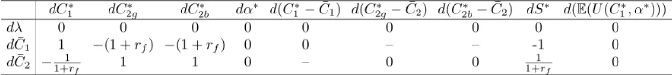
We summarize the results on the sensitivity analysis related to the solution presented in Proposition 2 in Table 2. It presents the changes of the first and second period optimal consumption, of the optimal investment in the risky asset, of the consumption gap in the first and second period, of optimal savings and of happiness (first row) with respect to changes in the loss aversion parameter and the first and second period consumption reference levels (first column).

dC

1^∗

dC

_2g^∗

dC

_2b^∗

dα

^∗

d(C

1^∗

− C ¯

1

) d(C

_2g^∗

− C ¯

2

) d(C

_2b^∗

− C ¯

2

) dS

^∗

d(E(U (C

1^∗

, α

^∗

)))

dλ 0 0 0 0 0 0 0 0 0

d C ¯

1

1 −(1 + r

f

) −(1 + r

f

) 0 0 – – -1 0 d C ¯

2

−

_1+r¹

f

1 1 0 – 0 0

_1+r¹

f

0

Table 2: Sensitivity results when aspirations are balanced (Ω = 0)

Similarly as for households with low reference levels an exogenous increase in the loss aversion parameter, keeping everything else constant, does not affect the solution. Note that now (Ω = 0) the household cannot set its first and second period reference levels indepen- dently from each other. So if we want to analyze the effect of an exogenous increase in the first period consumption reference level, for instance, we also have to consider the result- ing change (a decrease) in the second period consumption reference level. Taking this into consideration, an increase in the first period consumption reference will increase first period optimal consumption, will not affect risky asset holdings (they are always equal to zero) and will decrease (risk-free) savings. As less income is transferred to the second period, future consumption will in fact decrease in both states of nature. Following the same argument, an increase in the second period consumption reference level will increase the second period optimal consumption and reduce the first period consumption, since more (risk-free) savings have to be transferred to the second period. The consumption gap is equal to zero in both periods, so it is not affected by a change in either of the two consumption reference levels.

It can easily be seen that the indirect utility is not affected by either of the two consump- tion reference levels nor is it affected by the degree of loss aversion (as long as the household is sufficiently loss averse). I.e., the household’s level of happiness will be insensitive to an increase of the (first or second period) consumption reference level as well as to any changes of the degree of loss aversion.

Continuing our following the Joneses example (where the household sets its reference consumption level according to its neighbor’s consumption), the household actually mimics the Joneses behavior in the first or the second period, but not necessarily in both periods.

If this household sets its first period reference level according to the Joneses then C ₁ ^∗ =

C ¯ ₁ = C _1,Joneses ^∗ , so the optimal first period consumption levels of this household and of

the Joneses will be identical, and this household will follow the Joneses in the first period.

Since the two reference levels are tied together, however, this also means that C ₂ ^∗ = ¯ C 2 = (1 + r _f )(Y ₁ − C _1,Joneses ^∗ ) + Y ₂ , so this household’s reaction in the second period will be to decrease (increase) its optimal consumption provided the Joneses increased (decreased) their consumption in the first period. If, on the other hand, this household sets its second period reference level according to the Joneses, it mimics the Joneses in the second period in the following sense: it consumes exactly at the expected optimal consumption of the Joneses, namely, C ₂ ^∗ = ¯ C ₂ = E (C _2,Joneses ^∗ ), so this household will follow the Joneses in the second period. Again, since the reference levels are not independent, this means at the same time that ¯ C 1 = Y 1 + (Y 2 − E (C _2,Joneses ^∗ ))/(1 + r _f ) and hence the household’s reaction in the first period would be to decrease (increase) its optimal consumption provided the Joneses increase (decrease) their expected optimal consumption in the second period. In summary, our results imply that the balanced household follows the Joneses either in the first or in the second period but not in both, provided that the Joneses change their first and second period consumption in the same direction, i.e, increase – or alternatively decrease – their (expected) optimal consumption in both periods.

Some examples of reference consumption levels for Ω = 0

In the following we present some examples worth mentioning for the balanced household.

Example 5: C ¯ 1 = Y 1 and ¯ C 2 = Y 2

This situation occurs when the household sets its consumption reference levels equal to its respective incomes in both periods. In this case the household will invest neither in the risky asset nor in the risk-free asset, so no income is transferred to enable a larger future or current consumption. The household will totally consume its first period income in the first period and its second period income in the second period. Thus, households that belong to this category do not save or borrow anything and rely exclusively on their exogenous income to consume.

Example 6 (status quo): C ¯ ₂ = (1 + r _f )(Y ₁ − C ¯ ₁ ) and Y ₂ = 0

In this case, the second period consumption reference level is set equal to the gross return of investing the first period endowment income net of the first period consumption reference level which can be considered as the counterpart to reference levels in one-period models, which are equal to the gross return from investing all initial wealth into the risk-free asset. ¹⁶ In our case the initial wealth would correspond to Y ₁ − C ¯ ₁ . In addition, Y ₂ = 0, i.e., the household does not receive any exogenous second period income (as in one-period models).

16

See Hlouskova and Tsigaris (2012).

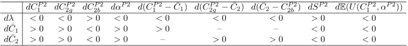
5 High reference values relative to endowment income (Ω < 0)

Now we consider the case when the household sets its consumption reference levels such that the present value is above the present value of its endowment income. This is done when the household has high aspirations. Let us first introduce the following notation

M ₁ (λ) = k

"

λ

^γ1

− 1

K _γ

¹_γ

#

(14)

˜

c ^{P 2} = (r g − r _b )(−Ω)

(r _g − r _f ) ¯ C ₂ (15)

C ¯ ₂ ^{P 2} = r _g − r _b

r _f − r _b (1 + r _f ) Y ₁ − C ¯ ₁ + Y ₂

(16)

δ ⁺ = 1 1 − p

r _g − r _f (1 + r _f )(r _g − r _b )

1−γ

(17)

k =

"

δ(1 + r _f )(1 − p)

r _g − r _b r _g − r _f

1−γ #

¹_γ

(18)

k 2 =

"

δ(1 + r _f )p

r _g − r _b r _f − r _b

1−γ #

¹_γ

(19) Note that M ₁ (λ) is an increasing function in λ and if λ ≥ _K ¹

_γ

then M ₁ (λ) ≥ 0. A simple derivation shows that λ > ^1+r _k

^f

+

1 K

γ

_γ¹

is sufficient for M ₁ (λ) > 1 + r _f . Note in addition that for ¯ C ₂ < C ¯ ₂ ^{P 2} is ˜ c ^{P 2} < 1.

We introduce an additional notation

λ ˆ =







 k ₂

1 + K

1

γ

γ

1 + r _f









γ

=







 k

1 +

1 K

γ

¹_γ

1 + r _f









γ

(20)

λ ^Ω<0 ₁ =







1+r

f

k +

1 K

γ

¹_γ

1 − ˜ c ^P2







γ

if ¯ C 2 < C ¯ ₂ ^{P 2} (21)

λ ^Ω<0 ₂ = ˆ λ



 C ¯ 1

Y 1 + ^Y _1+r

²

^{− C ¯}

²

f





γ

(22)

λ ˜ ^Ω<0 = 1 p



 1 δ

Y ₁ − C ¯ ₁ + _1+r ^Y

²

f

C ¯ ₂

! 1−γ

− (1 − p) 1 − ˜ c ^{P 2} λ ^Ω<0 ₁



 if ¯ C ₂ < C ¯ ₂ ^P2 (23)