Growth Effects of Consumption Jealousy in a Two-Sector Model

IHS Economics Series Working Paper 201

January 2007

Growth Effects of Consumption

Jealousy in a Two-Sector Model

Impressum Author(s):

Georg Duernecker Title:

Growth Effects of Consumption Jealousy in a Two-Sector Model ISSN: Unspecified

2007 Institut für Höhere Studien - Institute for Advanced Studies (IHS) Josefstädter Straße 39, A-1080 Wien

E-Mail: o ce@ihs.ac.atffi Web: ww w .ihs.ac. a t

All IHS Working Papers are available online: http://irihs. ihs. ac.at/view/ihs_series/

This paper is available for download without charge at:

https://irihs.ihs.ac.at/id/eprint/1749/

Growth Effects of Consumption Jealousy in a Two-Sector Model

201

Reihe Ökonomie

Economics Series

201 Reihe Ökonomie Economics Series

Growth Effects of Consumption Jealousy in a Two-Sector Model

Georg Duernecker

January 2007

Contact:

Georg Duernecker Department of Economics European University Institute

Villa San Paolo, Via della Piazzuola 43 50133 Florence, Italy

email: georg.duernecker@iue.it

Founded in 1963 by two prominent Austrians living in exile – the sociologist Paul F. Lazarsfeld and the economist Oskar Morgenstern – with the financial support from the Ford Foundation, the Austrian Federal Ministry of Education and the City of Vienna, the Institute for Advanced Studies (IHS) is the first institution for postgraduate education and research in economics and the social sciences in Austria.

The Economics Series presents research done at the Department of Economics and Finance and aims to share “work in progress” in a timely way before formal publication. As usual, authors bear full responsibility for the content of their contributions.

Das Institut für Höhere Studien (IHS) wurde im Jahr 1963 von zwei prominenten Exilösterreichern – dem Soziologen Paul F. Lazarsfeld und dem Ökonomen Oskar Morgenstern – mit Hilfe der Ford- Stiftung, des Österreichischen Bundesministeriums für Unterricht und der Stadt Wien gegründet und ist somit die erste nachuniversitäre Lehr- und Forschungsstätte für die Sozial- und Wirtschafts- wissenschaften in Österreich. Die Reihe Ökonomie bietet Einblick in die Forschungsarbeit der Abteilung für Ökonomie und Finanzwirtschaft und verfolgt das Ziel, abteilungsinterne Diskussionsbeiträge einer breiteren fachinternen Öffentlichkeit zugänglich zu machen. Die inhaltliche Verantwortung für die veröffentlichten Beiträge liegt bei den Autoren und Autorinnen.

Abstract

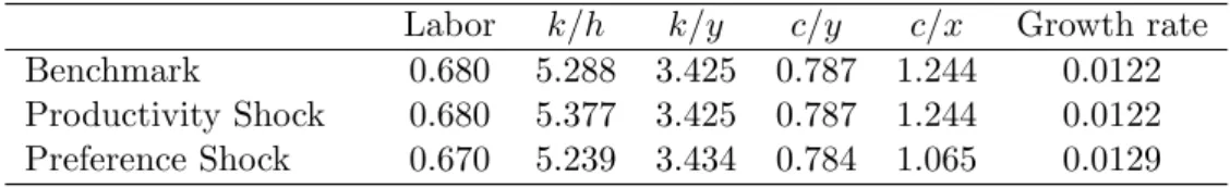
This paper aims at analyzing the implications of individuals’ consumption jealousy on the dynamic structure of a two-sector model economy. We find that status-seeking substantially influences both, the long-term properties and the adjustment behavior of the model.

Depending on the status motive, productivity disturbances might induce countercyclical responses of work effort whereas preference shocks are expected to generate an overshooting relative capital intensity. Generally we find that, for empirically plausible values of the intertemporal elasticity of substitution, a higher degree of consumption jealousy induces agents to devote more time to education which stimulates human capital accumulation and hence promotes economic growth.

Keywords

Status-seeking, economic growth, transitional dynamics, human capital

Comments

I am grateful to Walter H. Fisher, Juraj Katriak, and Martin Zagler for their very helpful discussions and suggestions. All errors that remain are entirely my own.

Contents

1 Introduction 1

2 The Model 4

2.1 Preferences ... 4

2.2 Technology and Accumulation ... 5

3 Equilibrium Analysis 6

3.2 Local Stability Analysis... 13

4 Transitional and Global Dynamics 15

4.2 The Set Up ... 16

4.3 Numerical Analysis ... 17

4.3.1 Case 1: Productivity Shocks ... 17

4.3.2 Case 2: Preference Shocks ... 21

5 Conclusion and Extensions 24

6 Appendix 26

1 Introduction

Time-separable utility representations have a long pedigree in economics and can be found at the core of most macroeconomic settings in recent work. Typically, an agent’s level of satisfaction is assumed to depend primarily on individual variables, like current consumption, leisure, or real money balances. There is, however, persuasive empirical evidence, some of which is provided by Oswald (1997), Frank (1997) and Fuhrer (2000) indicating that individual utility is to a large extent determined by comparing current variables like consumption or wealth to some specific standard, which is usually a given reference stock. This reference stock is typically assumed to comprise some measure of current and/or past economy-wide average consumption levels, which makes the utility representation time non-separable. The presence of this comparison element suggests that individuals derive utility from relative rather than absolute consumption.

Hence, they are concerned with their relative position in society, which is also referred to as their status. Generally, this type of preferences has been labeled as ”outward-looking” since agents base their decisions on an external comparison criterion

. The key issue of this paper addresses the implications of status seeking for the process of economic growth. The goal then, is to discuss whether - and if yes, to what extent - status, modeled as relative consumption exhibits a perceivable impact on the model’s equilibrium and transitional dynamics.

The idea that individuals’ choices are to some degree motivated by social rewards (including status) is in fact not a new one, but can be rather traced back to great thinkers such as Adam Smith (1776), Thorstein Veblen (1899) and David Hume (1978), among others. Nevertheless, a formal integration of this concept into economics was not until the work of Duesenberry (1949), who defined status as the ratio of an individual’s own consumption to average consumption of the others. Even though, time separability still plays a dominant role in economic modeling, there have been recent efforts to incorporate comparison utility into dynamic macro-settings.

For instance, in the field of asset pricing this concept has been invoked to explain certain asset pricing anomalies, such as the well-known equity premium puzzle raised by Mehra and Prescott (1985). Notable attempts in this regard have been made, for instance, by Constantinides (1990), Abel (1990) and Campbell and Cochrane (1999)

. Status orientation has also been successfully adopted to address issues of taxation. Ljungquist and Uhlig (2000) study the implications of a ”catching up” preference structure on short-run macroeconomic stabilization policies

. Liu and Turnovsky (2005) study the effects of consumption and production externalities on capital

1”Outward-looking” preferences are frequently referred to as ”Keeping/Catching up with the Joneses”, ”inter- dependent utility” or ”external habit formation”. There exists an alternative specification, which the literature has termed ”habit formation”, postulating an internal criterion as a comparison benchmark. In contrast to the

”outward-looking” case, the reference stock here depends on the agent’s own consumption history rather than the economy’s average.

2Constantinides (1990) employs a model with habit forming agents to address and resolve the premium puzzle, while Campbell and Cochrane (1999) analyze the effects of consumption externalities, induced by outward-looking preferences, on asset pricing and equity premiums. Gal´ı (1994) argues that ”keeping up” has the same effect as increasing the degree of risk aversion. This is due to the fact that consumers with these preferences dislike large swings in consumption, hence the premium paid for holding risky assets must be high relative to time separable preferences.

3They find that the optimal tax policy affects the economy countercyclically via procyclical taxes and, hence, mitigates aggregate demand fluctuations.

accumulation and welfare

. Comparison utility need not necessarily be defined over relative consumption. Various studies in the recent literature argue that it can be rather relative wealth that determines individuals status seeking. In the spirit of this approach Van Long and Shi- momura (2004) study the influence of wealth-inequality in a heterogeneous agents framework

. Recently relative wealth has also been studied by various authors in the context of open econ- omy settings. Most notably, Fisher (2004) and Fisher and Hof (2005) discuss an open economy Ramsey model that has been augmented by relative holdings of net foreign assets. They find that making allowance for status seeking can eliminate some crucial counterfactual properties of the conventional Ramsey model under time-separable utility

.

As mentioned at the outset, the time non-separable utility representation is strongly supported by empirical findings. Early studies by van de Stadt et al. (1985) confirm the hypotheses that an individual’s well-being depends on her relative position in society. Using panel data for the Netherlands they test for in- and outward-looking elements in individual utility. However, van de Stadt et al. (1985) cannot reject the existence of absolute and relative components. Fuhrer (2000) clearly rejects the time separable utility specification. He finds that both current aver- age consumption and an internal benchmark determine utility, where approximately 80% of the utility weight should be put on the latter. Moreover, Fuhrer and Klein (1998) argue that for G7 countries habit formation is a significant characteristic of people’s consumption behavior.

Interestingly, using data on British workers, Clark and Oswald (1996) provide empirical evidence that the level of individuals’ satisfaction is inversely related to comparison wage rates. Taking into account that wages, or, more precisely, income, is directly related to the consumption level of an individual, these results - along with the work carried out by Oswald (1997), Frank (1997) and Neumark and Postlewaite (1998) - are strongly in line with the theoretical predictions of the comparison consumption framework. The existing empirical evidence is admittedly sparse, but it nevertheless provides convincing support for the relevance of comparison elements in de- termining individual utility.

So far, relatively few papers have focused on the role status might play for economic growth.

Aside from early efforts by Ryder and Heal (1973) who incorporate habit formation into a neo- classical growth model it was not until the late 1990s that economists started to discuss status preference in the context of growth settings. Carroll et al. (1997) introduce two types of time non-separable elements - an internal and an external criterion - in a simple AK-framework and contrast the respective implications of each element on the model’s transitional dynamics

. A similar attempt has been made by Alvarez-Cuadrado et al. (2004), who discuss how alterna-

4The consumption externalities in their paper are again due to a preference structure that includes comparison elements. They derive an optimal tax structure that corrects for the distortions created by these externalities.

5They find that the initially poor might catch up with the rich if the marginal utility of relative wealth exceeds the elasticity of marginal utility of consumption. However, when people don’t care about their status, then the inequality will persist in the long run.

6Particularly the fact that an impatient economy - in the sense that the personal discount rate exceeds the world interest rate - mortgages all its wealth over time. They identified an endogenous effective rate of return that hinges on both own consumption and the net assets and ensures the existence of a long-run interior equilibrium, even if the discount rate exceeds the world interest rate.

7Observe that the conventional AK growth model exhibits no transitional dynamics. However, a modified preference structure that accounts for time non-separability alters this property.

2

tive assumptions about preferences affect the process of economic growth. They compare three different regimes, i.e. time separable, inward- and outward looking preferences and find that the departure from time-separability substantially alters the dynamic structure of the model.

Incorporating the concept of relative wealth in an endogenous growth setting, Futagami and Shi- bata (1998) find that if individuals are identical, higher status aspiration leads to higher growth whereas individuals’ heterogeneity might reduce growth through an induced misallocation of re- sources. Corneo and Jeanne (1997) assert that status orientation may lead to excessive growth resulting from an overaccumulation of physical capital, but it can also induce the social optimal rate of growth if the status aspiration is sufficiently strong. In a subsequent paper Corneo and Jeanne (2001) find that relative wealth incorporated into a neoclassical growth model - one that typically exhibits zero steady-state per capita growth - appears to be the engine of positive equilibrium growth. The vast majority of this work is primarily concerned with preference and demand-related issues hence the production side is rather oversimplified. But especially when addressing the dynamic process of economic growth one should be aware that - due to their one-sector design - AK or neoclassical modeling devices are rather restrictive.

The theoretical framework we employ accounts for the fundamental role human capital plays in explaining long-term growth of modern economies. Hence, in the spirit of Robert Lucas (1988) we choose a two sector production specification in which agents are assumed, first, to exhibit a certain degree of consumption jealousy. In other words, we assume that agents posses prefer- ences over their relative position in society. Second, individuals allocate their disposable time across the two production sectors to maximize their utility. This setting explicitly allows us to address a variety of issues that most of the existing literature fails to explain. For example, we can investigate the implications of consumers’ status seeking on the intersectoral allocation of productive resources, i.e. raw time, physical and human capital. Second to study how consump- tion jealousy affects the model’s transitional and equilibrium dynamics. This includes a careful discussion about the extent to which varying degrees of envy affect the adjustment behavior and the equilibrium growth performance. For the purpose of analyzing the dynamics, we con- sider specific productivity and preference shocks and numerically simulate adjustment paths of some selected key variables. Finally, we establish necessary and sufficient conditions that ensure the existence and the uniqueness of an interior equilibrium and show that these depend on the status-indicating parameters of the model.

Before closing this section we wish to stress some key-results of this analysis. First and foremost, we find that consumption jealousy substantially alters the dynamic structure of the economy.

Both in the balanced-growth equilibrium and during the transition the envy motive exhibits a non-negligible impact on the model’s key variables. For the equilibrium growth rate we ob- tain ambiguous effects of status seeking that mainly depend on the intertemporal elasticity of substitution. For parameter values that are in close accord with empirical estimates we find that productivity shocks in the final goods sector might induce (counter-)cyclical behavior of labor allocation resulting from an interplay of intersectoral reallocation and catching up efforts.

Preference shocks, in contrast, entail a monotonous response of labor but cause an overshooting

long-run capital intensity. This can be traced back to interdependencies of temporary pro-

ductivity imbalances across sectors and the average product of physical capital, in response to that shock. Generally we can state that a higher degree of status seeking tends to increase the schooling efforts and hence stimulates economic growth. Moreover, there exists a unique interior balanced growth path equilibrium whose properties depend to a large extent on the parameters that determine the envy motive.

The remainder of the paper is organized as follows. In Section 2 we lay out the basic structure of the theoretical model introducing a time non-separable preference representation. Section 3 derives the equilibrium conditions and discusses the necessary and sufficient conditions for exis- tence and uniqueness of a balanced growth equilibrium. This section also contains a stability and sensitivity analysis that underlies the local saddle path stability of the model. Section 4 studies the off-equilibrium dynamics of the economy which is mainly done by numerical simulation.

Section 5 concludes and discusses possible extensions.

2 The Model

2.1 Preferences

As a basic framework we consider a two-sector model economy populated by a continuum [0, 1] of identical atomistic individuals with unbounded horizon. Let agent i’s utility at each point in time depend on the comparison of her own consumption, c

(t), to a certain reference stock which in this model is determined by the average level of consumption in the economy, ˜ c(t) = R

0

c

(t)di.

In particular, preferences of agent i are characterized by a C

utility function U (c

(t), ˜ c(t)) satisfying the standard concavity and limiting-behavior properties in c, i.e. U

(·) > 0, U

(·) < 0 and lim

U

(·) = +∞, lim

U

(·) = 0.

To be more concrete, the functional form of U (c

(t), ˜ c(t)) in this paper is postulated to be isoelastic which will allow us to derive explicit results.

U (c

(t), c) = (1 ˜ − σ)

c

(t)(κ Z

0

e

˜ c(s)ds)

(1) Each individual discounts the utility of her future consumption at a constant exogenously given rate ρ ≥ 0 and let σ > 0 denote the inverse of the intertemporal elasticity of substitution

. Furthermore, in accordance with much of the existing literature on status preferences, it is assumed that individuals, in general, envy their neighbors consumption, hence U

(·) < 0 and U

(·) > 0

. The latter condition implies that an agent values an additional amount of own consumption more, the higher the average level of consumption in the economy is. The reference stock, call it x(t), is composed of the weighted sum of current and past average consumption levels, i.e. x(t) = κ R

0

e

˜ c(s)ds where κ ∈ [0, ∞) indexes the relative importance of recent compared to past average consumption. A more intuitive interpretation of κ can be deduced

8Similar versions of (1) have been recently used, for instance by Alvarez-Cuadrado et al. (2004) and Carroll et al. (1997).

9The case of admiration that is characterized by Uc˜(·)>0 is considered by Dupor and Liu (2003) and Liu and Turnovsky (2005)

4

from the dynamic representation of x(t). Using Leibnitz’ rule we get ˙ x(t) = κ (˜ c(t) − x(t))

from which we can infer that κ drives the speed of adjustment of the reference stock. For high values of κ adjustment is rather rapid implying that x(t) is close to ˜ c(t) with lim

x(t) = ˜ c(t).

In this case individuals preferences are more presence-orientated. On the other hand, extremely low values of κ lead to sluggish adjustment and hence x(t) hardly varies. Moreover, it should be mentioned that the two polar cases, i.e. κ → 0, ∞, nest important classes of economic models.

First, for sufficiently high values of κ we have x(t) ≈ ˜ c(t) and, as a consequence, all that matters for an agent’s utility is the current average consumption level in the economy. For this type of preference structure the recent literature has coined the expression ”Keeping up with the Joneses”

. Second, κ → 0, hence x(t) ≈ x(0), ∀t ∈ (0, ∞), implies that the reference stock is irrelevant to an agent’s utility and as a result U (·) collapses to the standard time-separable utility representation. The cases implied by values of κ lying in between these extremal points, often called ”Catching up with the Joneses”, will be the main focus of this paper. The importance of comparison utility for an agent’s well-being is governed by the parameter β ∈ [0, 1]. For β = 0 comparison utility is all that matters while if β = 1 individuals only care about their own absolute consumption. In case of β ∈ (0, 1) both are attached with strictly positive utility.

Due to the fact that the reference stock is solely determined by ˜ c(t), preferences are by definition outward-looking

. Moreover, individuals take the path of x(t) as given when making their allocative decisions. This inevitably creates a negative externality since agents do not take into account the effects of their own choices on the current and future reference stock of the others.

2.2 Technology and Accumulation

The model economy considered in this paper comprises two sectors: a final goods sector pro- ducing a single, homogeneous, non-storable consumption good and an education sector creating additional human capital. Each agent is endowed with one unit of time. Let χ

and χ

denote the fraction of time individual i devotes to work in the goods sector and uses for edu- cational purposes, respectively. For sake of simplicity leisure is not considered in this model, hence notation can be simplified by writing χ

= χ

and χ

= (1 − χ

). In each point in time an individual’s final output y

(t) is determined by the stock of her accumulated physical, k

(t), and human capital, h

(t), and the level of raw labor according to a constant returns to scale technology

y

(t) = φk

(t)

(χ

(t)h

(t))

, (2)

10In this paper we denote ˙q(t)≡ ^∂q(t)_∂t

11This specification of agents’ preferences has found widespread use, for instance, in work concerned with asset pricing, (see Gal´ı (1994)), taxation, (see Ljungquist and Uhlig (2000)), and open economy issues, (see Fisher (2004) and Fisher and Hof (2005)), to mention a few. Dupor and Liu (2003) go a step further and distinguish between

”Jealousy” and Keeping up with the Joneses. For an increase in aggregate consumption the first is associated with a lower level of individuals utility whereas in the latter environment the marginal utility of individual consumption rises relative to that of leisure.

12This is in contrast to inward looking behavior that constitutes the basis for the concept of habit formation.

It makes use of the assumption that agents’ own past consumption builds a habit typed reference stock.

13For future reference note that ”time” and ”raw labor” are used interchangeably.

with α ∈ (0, 1) and φ > 0 denoting a technology shift parameter. Given that h

reflects the efficiency per unit of raw labor supplied, χ

h

clearly signifies the amount of effective labor used in the goods production. Final output can be either consumed currently or saved and transformed into physical capital

k ˙

(t) = φk

(t)

(χ

(t)h

(t))

− c

(t) − δk

(t), (3) where δ ≥ 0 denotes the constant, exogenously given, capital depreciation rate. The educa- tion sector utilizes human capital together with time to produce new human capital. In light of recent empirical evidence I refrain from using the traditional assumption that the human capital growth rate is linear in time. As pointed out by Alonso-Carrera (2001), results from life-cycle earnings estimations strongly suggest strict concavity of the accumulation technology in schooling time, implying diminishing private returns to education. Accounting for this fact the human capital accumulation technology is postulated to be

h ˙

(t) = ϕ (1 − χ

(t))

h

(t) − ηh

(t), (4) with constant and exogenous parameters ϕ > 0, η ≥ 0 and ζ ∈ (0, 1).

3 Equilibrium Analysis

In a decentralized economy each agent i faces the following problem max

(ci(t),χi(t))

Z

U (c

(t), c(t)) ˜ e

dt, (5) subject to

k ˙

(t) = φk

(t)

(χ

(t)h

(t))

− c

(t) − δk

(t), h ˙

(t) = ϕ (1 − χ

(t))

h

(t) − ηh

(t),

c

(t) ≥ 0 k

(t) ≥ 0 h

(t) ≥ 0, χ

(t) ∈ [0, 1] , ∀t ∈ [0, ∞) , k

(0) = k

h

(0) = h

,

(6)

taking the path of x(t) ≥ 0 as given. Equations (5)-(6) denote a common dynamic optimiza- tion problem with control variables c

(t) and χ

(t) and state variables h

(t) and k

(t). From the maximum principle we get a system of first-order necessary conditions for optimality

c(t)

x(t)

− π(t) = 0, (7)

(1 − α) π(t) φk(t)

(χ(t)h(t))

χ(t) − λ(t)ϕζh(t) (1 − χ(t))

= 0, (8)

6

−π(t) αφk(t)

(χ(t)h(t))

k(t) − δ − ρ

!

= ˙ π(t), (9)

−π(t) (1 − α) φk(t)

(χ(t)h(t))

h(t) − λ(t)

ϕ

1 − χ(t)

− η − ρ

= ˙ λ(t). (10)

The impact of consumption jealousy is clearly reflected by (7) that equates costs and benefits of an additional unit of own consumption. A higher reference stock or a higher degree of jealousy (reflected by a lower β) pushes-up the marginal utility of consumption, implying that an additional unit becomes more valuable. Given the fact that the Hamiltonian function associated with (5)-(6) is jointly concave in both choice variables c and χ the first order conditions are not only necessary but also sufficient for optimality if, in addition, the following transversality conditions are fulfilled

t→∞

lim e

π

(t)k

(t) = 0, lim

t→∞

e

λ

(t)h

(t) = 0.

The terms π and λ denote the co-state variables associated with the physical and human capital stock, respectively. In order to get a clear picture of the equilibrium concepts used in the subsequent analysis, it is quite instructive to state the following definitions.

Definition 1 A symmetric perfect-foresight equilibrium consists of paths {c(t), χ(t), k(t), h(t), x(t)}

that solve the optimal control problem indicated in (5)-(6) for given initial condi- tions k(0) = k

, h(0) = h

.

Note that this definition already accounts for the fact that due to agents’ symmetry in preferences and endowments we have ˜ c = c

= c and χ

= χ.

Definition 2 A balanced growth path equilibrium (BGP) is a set of paths {c(t), χ(t),

k(t), h(t), x(t)}

satisfying Definition 1 such that c(t), k(t), h(t), x(t) grow at a constant rate and χ(t) is constant.

The optimality conditions together with the laws of motion for k, h and x can now be combined yielding a five-dimensional system that fully describes the underlying dynamics of the model economy

γ

=

αφχ(t)

ξ(t)

− δ − ρ − (1 − β) (1 − σ) κ (ω(t) − 1)

σ

, (11)

14In order to facilitate the analysis and to reduce notational clutter we define the following ratios that are constant along the BGPω=c/x,ν=c/kandξ=k/h. Furthermore, we useγq≡^q_q^˙.

γ

=

−αν + ϕ (1 − χ(t))

1 − χ(t) (1 − ζ ) 1 − χ(t) − α

+ (1 − α) (δ − η)

α + (1 − ζ) χ(t) 1 − χ(t)

,

(12)

γ

= φχ(t)

ξ(t)

− ν (t) − δ, (13)

γ

= ϕ (1 − χ(t))

− η γ

= κ (ω(t) − 1) . (14) Applying Definition 2 to the system above, we can immediately conclude that the key vari- ables not only grow at a constant, but also common rate given by

γ

= γ = αφ (χ

/ξ

)

− δ − ρ

1 − β (1 − σ) , (15)

and implying, γ

= γ

= γ

= γ

= γ

≡ γ . Before we continue our steady state analysis let us stop at this point and take some time to reflect on the implications of (15). At a first glance the equilibrium growth rate looks similar to the well-known Keynes-Ramsey rule in the conventional Uzawa-Lucas two sector growth model. For comparison reasons let us denote it by γ

. The numerator reflects the difference between the net marginal product of capital and the discount rate. However, the denominator makes the crucial difference. For values of the intertemporal elasticity of substitution sufficiently large implying σ < 1 and for β ∈ (0, 1) it is always true that γ

> γ. However, for empirically plausible values of σ, i.e. σ > 1 we get the reverse case, γ

< γ. In addition, this relationship becomes more pronounced the higher agents value status, i.e. for lower values of β. To develop the economic intuition underlying this dependence, we need to go deeper into the steady state analysis. First, for convenience, we rewrite the dynamic system in (11)-(14) using the ratio-definitions

γ

= h

αφχ(t)

ξ(t)

− δ − ρ − [1 − β (1 − σ)] κ (ω(t) − 1) i

σ

, (16)

γ

= h

φχ(t)

ξ(t)

− ν(t) − δ − ϕ (1 − χ(t))

+ η i

, (17)

γ

= h

φ (χ(t)/ξ(t))

(α − σ) − (1 − σ) [(1 − β) κ (ω(t) − 1) + δ] + ν(t)σ − ρ i

σ

, (18)

γ

=

−αν + ϕ (1 − χ(t))

1 − χ(t) (1 − ζ ) 1 − χ(t) − α

+ (1 − α) (δ − η)

α + (1 − ζ) χ(t) 1 − χ(t)

.

(19)

8

Next, we assume that an interior BGP exists

.

Definition 3 An interior balanced growth path equilibrium is a set of paths {c(t), χ(t), k(t), h(t), x(t)}

satisfying Definition 2 and 0 < χ(t) < 1 −

η ϕ

ζ

∀t ∈ [0, ∞).

Note that Definition (3) implies two things; first an interior BGP can only exist if both sectors are active and second, the equilibrium growth rate is strictly positive, implying endogenous growth. Ad hoc activity could in principle be ensured by the weaker condition χ ∈ (0, 1) but the case χ ∈

1 − (η/ϕ)

, 1

would not be sustainable since it implies ˆ h(t) < 0 resulting in lim

h(t) = 0 and a shutdown of the goods sector.

Recall that by definition ˙ ν (t) = ˙ ξ(t) = ˙ ω(t) = ˙ χ(t) = 0 must hold along an interior balanced growth path. Consequently, after setting (16)-(19) equal to zero we get, after a fair amount of algebra, a system {ν

(χ

) , ξ

(χ

) , ω

(χ

) , χ

} that implicitly determines the equilibrium values of the corresponding variables

.

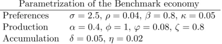
To get a clear-cut picture of the steady state’s quantitative properties, we calibrate the system and compare the results to features of actual economies. The parametrization we employ is compactly summarized in Table (1).

Parametrization of the Benchmark economy Preferences σ = 2.5, ρ = 0.04, β = 0.8, κ = 0.05 Production α = 0.4, φ = 1, ϕ = 0.08, ζ = 0.8 Accumulation δ = 0.05, η = 0.02

Table 1: Benchmark Parameters

The conventional preference and technology parameters are set in accordance with the lit- erature, see e.g. Mulligan and Sala-i-Martin (1993) and Ortigueira and Santos (2002), Lucas (1990), Gong et al. (2004). Moreover, κ is chosen to fit plausible rates of convergence while the value of β is set such that both, absolute and relative consumption are attached with positive utility. Table (2) provides some rough impression about the features of the resulting benchmark economy.

χ

c^∗

y^∗

ι

γ

0.680 5.288 3.425 0.787 0.056 0.0122

Table 2: Benchmark Economy

In fact, the results in Table 2 fit actual economic data remarkably well. Since the model abstracts from population growth, aggregate values are associated with per capita values. In light of this an equilibrium growth rate of 1.2% per annum seems to be quite plausible. The

15The proof of existence and uniqueness is provided below.

16The equilibrium expressions can be found in the appendix. Notice that a^∗attached to a variable denotes its steady-state value.

capital-output ratio taking a value of 3.4 is very close to results obtained by Alvarez-Cuadrado et al. (2004) and Eicher and Turnovsky (2001). Furthermore, the derived value of the consumption- output ratio indicates that almost 79% of final output are devoted to individuals consumption.

In this case Alvarez-Cuadrado et al. (2004) obtain a similar result. Given that we neglect governmental activities, this value appears to be highly plausible. In addition, Table 2 attests that individuals engage for slightly less than one third of their disposable time in education.

Accounting for the fact that the concept of education used in this paper includes all sorts of human capital accumulation - not only formal schooling but also activities such as acquiring job specific skills and knowledge, learning by doing or on the job training - the seemingly low value in Table 2 turns out to be quite realistic. The capital stocks ratio indicates that in equilibrium the physical capital stock of the economy is more than 5 times higher than its human capital stock.

Finally, ι

which is the eigenvalue that satisfies 0 > ι

> ι

implies that the asymptotic speed of convergence of the economy is around 5.6% per annum. This value exactly lies in the consensus range of 3% −11% implying a high degree of empirical consistency. On the whole, the remarkable fit of the indicated equilibrium features to the characteristics of actual economies makes us highly confident of the model’s ability to generate also realistic and insightful transitional dynamics.

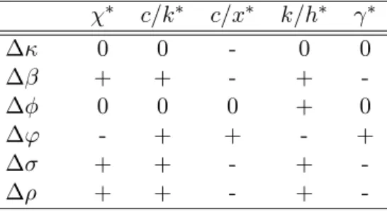
Using these results we can conduct some comparative statics analysis by computing the effects of parametric changes on the equilibrium values. These results are displayed in Table 3 below.

χ

c/k

c/x

k/h

γ

∆κ 0 0 - 0 0

∆β + + - + -

∆φ 0 0 0 + 0

∆ϕ - + + - +

∆σ + + - + -

∆ρ + + - + -

Table 3: Effects of parametric changes on equilibrium values

Notice that the table also includes the equilibrium growth rate. The impact of the conven- tional technology and preference parameters φ, ϕ, σ and ρ are fairly standard and well docu- mented and interpreted by earlier studies, see e.g. Mulligan and Sala-i-Martin (1993). However, a thorough analysis on the influence of both new parameters β and κ, reflecting, respectively, individuals’ desire for social status and the persistence of past average consumption, has been lacking, as of yet, in an endogenous growth environment.

The effects of κ on the model’s steady-state values are not dramatic. Only the status-indicating variable ω responds to changes in κ which is, after recalling the definition of ω, self-explanatory.

An increase in κ leads to faster adjustment of the reference stock, which in the limit approaches

˜

c. Since ˜ c = c due to symmetry, we have lim

ω(κ) = 1. Despite modest steady-state effects, κ nevertheless plays a crucial role in determining the model’s off-equilibrium behavior, as we will see later on. In contrast, the impact of β on the model’s equilibrium is far more complex. As indicated in the second row of Table 3, a lower degree of consumption enviousness leads to a higher equilibrium final good employment, consumption-capital ratio, and physical to

10

human capital ratio, whereas the steady state growth rate and relative consumption experience a decline. The economic intuition behind these phenomena can be best elucidated using the agent’s optimality conditions with respect to consumption, (7), and the state variable k, (9).

Given the fact that (∂U

/∂β) < 0, we can conclude that an incremental increase in β lowers the marginal utility of own consumption, which, as implied by the optimality condition, leads to a drop in the shadow value of capital. As a consequence, its (negative) growth rate is stimulated.

The reestablishment of equality in equation ˆ π(t) = −M P K(t) + δ + ρ, that results from the agent’s first order conditions, requires an increase in the marginal product of capital (M P K) which is achieved by a sufficiently large increase in activity in the final goods sector, χ. Since we have (∂ξ

(χ

)/∂χ

) > 0, ∀χ ∈

0, 1 − (η/ϕ)

, the physical to human capital ratio, ξ

increases but by less than χ is rises, i.e. ∆χ > ∆ξ

. This yields the required condition

∂

ξ^∗

/∂χ

> 0 which causes the final rise in the marginal product. As shown in Table 3, the long run growth impact of a higher β is clearly negative. Note that a rise in β in fact entails two opposing effects on the equilibrium growth rate, which becomes clear by inspecting equation (15). An indirect positive effect is triggered by the higher steady state marginal product of phys- ical capital which enhances the numerator of (15) and, as a result, also growth. Weaker status motives, on the other hand, also create a direct growth depressing effect. As can be inferred from the human capital accumulation technology (4), the induced intersectoral reallocation of time toward final goods production impacts growth in a negative way. For future reference, let’s de- note these effects by ”marginal product effect” and ”reallocation effect”, respectively

. For the parametrization used above we get that the negative reallocation effect outweighs the positive marginal product effect which finally results in the indicated negative overall effect. However, the picture changes substantially when we vary the value of σ around one. In particular, if σ is small enough, i.e. σ < 1, the signs in the second row of Table 3 are reversed, indicating the opposite effects as described above. This leads us directly to our first result.

Result 1 For σ ∈ (0, 1) (respectively σ ∈ (1, +∞)) a lower degree of consumption jealousy, i.e. a higher value of β, implies that the reallocation effect is positive (negative) and stronger (weaker) than the negative (positive) marginal product effect, resulting in an overall positive (negative) impact on the equilibrium growth rate. For the knife edge case, σ = 1, changes in the status motive have no impact on equilibrium allocations and growth.

Furthermore, the positive response of the consumption-capital ratio, ν

depicted in Table 3 is intimately connected to the increase in labor since (∂ν

(χ

)/∂χ

) > 0. Finally, it remains to explain the negative impact of weaker status motives on relative consumption. In fact, this turns out to be pretty straightforward. Rearranging the instantaneous utility function given in (1) to explicitly model the status dependence yields U (c(t), ω(t)) = (1 − σ)

c(t)

ω(t)

,

17This result can be established using the steady state value ofξ^∗, see equation (27) in the appendix. Values ofχoutside this range would not fulfill this condition but since we are considering only interior equilibria we can omit them.

18To be precise, themarginal product effectin this paper generally denotes the positive stimulus for consumption growth caused by a higher marginal product of capital. It is, therefore, equivalent to what Alvarez-Cuadrado et al. (2004) call therate of return effect.

from which we can infer that for an increasing β the benefit of an additional unit of relative consumption declines steadily, i.e. ∂U

/∂β < 0. A low marginal utility of ω, caused by a high β, induces agents to accumulate less of it which finally results in the negative response displayed in Table 3. This section can be concluded by stating another important result.

Result 2 An economy that awards an agent’s level of consumption with social status devotes more time to education and as a consequence exhibits a relatively higher human than physical capital stock than an economy with weaker or no status valuation.

3.1 Existence and Uniqueness of a Steady State Equilibrium

For notational convenience, let us first define m ≡ 1 − (η/ϕ)

and Ξ = {χ ∈ < : 0 < χ < m}.

To establish existence of an interior equilibrium, we need to find a χ ∈ Ξ that solves the system {ν

(χ

) , ξ

(χ

) , ω

(χ

) , χ

}. For this purpose we define the function F : [0, 1) → < using the implicit equilibrium expression for χ

.

F (χ) = ϕ (1 − χ)

[ζχ + β (1 − σ) (1 − χ)] − ρ − βη (1 − σ) (20) Any χ that solves F (χ) = 0 and satisfies χ ∈ Ξ is a candidate for an interior equilibrium.

This leads us to the following proposition.

Proposition 1 If β (1 − σ) (ϕ − η) < ρ < ζη

1−m

, then there exists a unique χ

∈ Ξ such that the quadruple (ν

(χ

), ξ

(χ

), ω

(χ

), χ

) constitutes an interior balanced growth path equi- librium.

Proof. The proof itself is straightforward. Notice that F (χ) is at least twice continuously differentiable for all χ in the domain. As a first step we have to check the properties of the function F (χ) at the boundaries, i.e. lim

F (χ) and lim

F (χ). For these we get

χ→0

lim F (χ) = β (1 − σ) (ϕ − η) − ρ, and

χ→m

lim F (χ) = ζη ϕ

η

− 1

!

− ρ.

Another important ingredient is the slope of F (χ).

F

= ϕζ (1 − χ)

1 − χζ

1 − χ − β (1 − σ)

Since

(1−χ)^1−ζ

> 0 and

≥ 1, ∀χ ∈ [0, 1), we see that F

> 0, ∀χ ∈ Ξ. The picture that emerges from this exposition suggests that F (χ) is a strictly increasing function ∀χ ∈ Ξ.

Accounting for this fact, the proof essentially reduces to verifying that ∃χ ∈ Ξ such that F (·) = 0. Since F (·) is strictly increasing, it is clearly the case that an interior equilibrium can exist iff F (0) < 0 and F (m) > 0. From the limiting behavior properties of F (χ), we can infer that the

12

necessary and sufficient conditions for these cases are σ > 1−

and ζη

ϕ η

ζ

− 1

−ρ > 0.

After some simple rearrangement, we obtain the condition used in Proposition 1. To finalize the proof, note that the solution candidate needs to fulfill both transversality conditions. We know that in the limit the transversality conditions can be expressed as −ρ + γ

+ γ

< 0 and

−ρ + γ

+ γ

< 0. Using (9) and (10) yields

− χ(t)

(1 − χ(t))

< 0, and

− αϕζχ(t)

(1 − χ(t))

< 0,

which both hold for all χ ∈ Ξ. As a result, we can conclude that an interior balanced growth equilibrium exists if both conditions σ > 1 −

and ζη

ϕ η

− 1

− ρ > 0 are satisfied.

Furthermore, uniqueness is given by the fact that F (χ) is strictly increasing and, hence, the F (χ) = 0 line can be crossed only once.

3.2 Local Stability Analysis

The local stability properties of an equilibrium can, in general, be studied by analyzing the structure of the eigenvalues of the dynamic system that has been linearized around its steady state. For this purpose we take the fourth-order dynamic system in (16)-(19) and apply first order Taylor expansions to approximate the models dynamics













˙ ω ξ ˙

˙ ν

˙ χ













=













−ω^∗κ[1−β(1−σ)]

σ

j

0 −

j

0 j

−ξ

ξ

σ

ω^∗α

j

+

j

−ν^∗(1−σ)(1−β)κ σ

ν^∗(α−σ)

ω^∗α

j

ν

−

j

0 0 j

ζϕ (1 − χ

)

χ

























∆ω

∆ξ

∆ν

∆χ













. (21)

For tractability, we define, j

= − (1 − α)

ν

+ δ + ϕ (1 − χ

)

− η ,

j

= −ω

αφ (1 − α) (χ

/ξ

)

(ξ

σ)

, j

=

and ∆ω = ω−ω

. The terms j

denote the matrix element in the mth row and nth column. To check the local stability properties of the system it would, in principle, be sufficient to determine the signs of the eigenvalues of the Jacobian. Doing this in an analytical way can be quite challenging, however. A proper way to circumvent difficulties that are due to a high degree of complexity is to solve for sign-indicating conditions, i.e. conditions from which one can draw conclusions about the properties of the eigenvalues and hence the stability of the system

. Nevertheless, solving for these conditions in

19In the case of a two dimensional system these conditions are simply the trace and the determinant of the corresponding Jacobian matrix, while in a three-dimensional system the termj12j22+j13j31+j23j32−j11j22− j11j33−j22j33<0 is an additional condition.

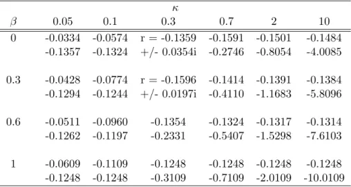
our fourth-order system turns out to be intractable as well. An elegant way out is to evaluate the roots by calibrating the model’s structural parameters with precise values. The strategy that is adopted in this procedure, however, accounts for the fact that the literature is sparse about precise or even the range of values of non-conventional preference parameters such as β and κ. This problem is tackled by simply computing the models eigenvalues for a broad range of possible values of β and κ, while the remaining parameters are set in accordance with the empirical literature. Results are reported in Table 4 below. Notice that the table contains only the negative eigenvalues.

κ

β 0.05 0.1 0.3 0.7 2 10

0 -0.0334 -0.0574 r = -0.1359 -0.1591 -0.1501 -0.1484 -0.1357 -0.1324 +/- 0.0354i -0.2746 -0.8054 -4.0085 0.3 -0.0428 -0.0774 r = -0.1596 -0.1414 -0.1391 -0.1384 -0.1294 -0.1244 +/- 0.0197i -0.4110 -1.1683 -5.8096 0.6 -0.0511 -0.0960 -0.1354 -0.1324 -0.1317 -0.1314 -0.1262 -0.1197 -0.2331 -0.5407 -1.5298 -7.6103 1 -0.0609 -0.1109 -0.1248 -0.1248 -0.1248 -0.1248 -0.1248 -0.1248 -0.3109 -0.7109 -2.0109 -10.0109 Note: the remaining parameters are the same as in Table 3

Table 4: Asymptotic Speed of Convergence

This simple calibration exercise indeed sheds some light on the structure of the eigenvalues.

As clearly indicated in Table 4, the system possesses two stable and two unstable eigenvalues, from which we can deduce the existence of local saddle path stability

. Recalling, however, that for parameter values with less empirical support the model might display contrary stability features, we deal the subsequent analysis with great care. Notice that apart from stability consid- erations, the eigenvalues in Table 4 can also be consulted to draw conclusions on the asymptotic speed of convergence of the model’s variables. In principle, we know that the asymptotic behav- ior of a m-dimensional dynamic system exhibiting saddle path stability is essentially governed by the eigenvalue ι

that satisfies 0 > ι

> ι

> ... > ι

. From Table 4 we can infer that the displayed eigenvalues ι

with ι

> ι

span a range of −0.033 to −0.15, indicating that the economy asymptotically converges at rates of 3% to 15% per annum toward its steady state. The empirical evidence on the adjustment speed is, in fact, far from being in unison. Early studies in this field (see e.g. Barro and Sala-i-Martin (1992)) found values around 2% per annum whereas more recent results suggest annual rates up to 11% (e.g. Islam (1995) and Caselli et al. (1996)).

Our model perfectly matches these results for the whole range of β and sufficiently low values of κ, i.e. κ < 0.3. High values of κ appear to be implausible, since they would imply rates of convergence up to 16%.

20Observe that for selected combinations of parameters we get complex roots indicating cyclical behavior of the system.

14

4 Transitional and global dynamics

4.1 The Benchmark Economy

Having conducted a fruitful equilibrium and stability analysis, we now concentrate our attention to the characterization of the model’s behavior outside the steady state. The transitional dy- namics in one-sector neoclassical and two-sector endogenous growth models is now, in general, well understood thanks to insightful studies by Mulligan and Sala-i-Martin (1993), Bond et al.

(1996) and Eicher and Turnovsky (2001), to mention just a few. Nevertheless the importance of transition in the recent literature is generally underestimated and, hence, carelessly handled.

As a result, the focus of numerous studies is on balanced growth properties only, without paying sufficient attention to the off-equilibrium behavior. This is problematic insofar as, first, the authors implicitly or even explicitly assume existence of a steady state without ensuring that the economy actually converges to an equilibrium at all. And second, as shown by Mulligan and Sala-i-Martin (1992), periods of transition can be rather long implying that off-equilibrium conditions might have a substantial quantitative impact on the overall economic performance.

Noteworthy exceptions to this practice are Alvarez-Cuadrado et al. (2004), Alonso-Carrera (2001) and Caballe and Santos (1993). The stability analysis above indeed gives rise to the con- jecture that transitional dynamics might play a substantial role in our model. Given that the conditions for saddle path stability are satisfied the off-equilibrium dynamics is governed by two negative eigenvalues so that the stable manifold is two-dimensional

. As pointed out by Eicher and Turnovsky (2001), a two-dimensional transition path substantially enriches the model’s dynamics by introducing additional flexibility that allows its behavior to mimic important fea- tures of economic data. They mention that as a direct consequence of a higher dimensional adjustment locus the speed of convergence might differ across variables, which permits a more flexible time path

. Moreover, adjustment paths need not be monotonic. Since the dynamics is determined by two negative eigenvalues, their respective influence on the adjustment is subject to variations as time proceeds implying also the possibility of overshooting. Finally, systems with two or higher dimensional stable manifolds might respond asymmetrically to positive or negative shocks of equal magnitude. This is in clear contrast to conventional one-sector growth models in which the response to a positive shock is just the mirror image of the same nega- tive shock (Eicher and Turnovsky, 2001). To study the transitional dynamics in our model, we assume that the system summarized in (16)-(19) is initially in equilibrium. Thereafter, we confront the model by specific shocks and trace out the subsequent time path of some selected key variables. The strategy we adopt therein implicitly makes use of the fact that due to the

21The stable manifold is the locus of points from which the respective variables asymptotically converge to their equilibrium values if they are allowed to evolve according to their laws of motion. In the well-known Ramsey optimal growth model, for instance, the stable manifold is one-dimensional implying that for each value of k (physical capital) there exists a uniquec(consumption) that places the economy on the stable arm of the saddle path. The same applies to most classes of one-sector growth models including theAKmodel.

22More precisely, this allows variables to evolve virtually independently from the time path of other variables. In their paper, Eicher and Turnovsky (2001) consider a two-sector non-scale growth model that permits technology and physical capital to evolve independently and at different adjustment speeds that is consistent with empirical evidence.

local stability characteristics, the economy returns to the BGP equilibrium after it was hit by a shock. Consequently, after implementing a specific disturbance, we can numerically simulate the time path of selected variables to reproduce the transitional dynamics until the economy reaches the equilibrium path again

.

4.2 The Set Up

Given that the transitional adjustment locus is a two-dimensional stable saddle path, we can express the stable solution of (16)-(19) in terms its eigenvalues and -vectors. This enables us to separate the interdependent system and get self-contained equations, which greatly facilitates the subsequent analysis. In particular, making use of the two stable roots denoted by ι

, with ι

< ι

< 0, and the associated normalized eigenvectors, υ

= (υ

, 1, υ

, υ

)

, we can reformulate the generic form of any two variables in (16)-(19) to explicitly express their time path during transition.

ω(t) = ω

+

(ω

− ω

) υ

e

− υ

e

− (ξ

− ξ

) υ

υ

e

− e

(υ

− υ

)

(22)

ξ(t) = ξ

+

(ω

− ω

) e

− e

− (ξ

− ξ

) υ

e

− υ

e

(υ

− υ

)

(23) For expositional convenience, we depict here only the path of the capital stocks ratio, ξ and comparison consumption ω

. However, the remaining ones, i.e. for χ and ν, can be established analogously. From (22) we can immediately infer that if t → +∞, ω(t) = ω

. The same, of course, applies to ξ, χ and ν implying that the economy asymptotically returns to its equilibrium path. However, this adjustment behavior need not be monotonous. The off-equilibrium dynamics of the variables under scrutiny can now analytically be approximated by

˙ ω(t)

ξ(t) ˙

!

= 1

υ

− υ

υ

ι

− υ

ι

υ

υ

(ι

− ι

) ι

− ι

υ

ι

− υ

ι

! ω(t) − ω

ξ(t) − ξ

!

. (24)

It might come as surprise that the original interrelated fourth-order system expressed in (16)-(19) can be reduced to two-dimensional systems without loosing any feedback information coming from the respective isolated variables. Or to state it more clearly, why should the original interdependence of ξ and χ in (16)-(19) be decoupled and simply disappear? Concerning this issue, Eicher and Turnovsky (2001, p.97, footnote 13) point out that despite there is no apparent link between the imbedded and the detached variables the system takes fully account of the feedback namely through the two eigenvalues. As a result, the dynamics expressed in

23Notice that the equilibrium is in fact reached whent→+∞, hence the simulation is just an approximation, even though a very precise one.

24Notice that equations (22)-(23) can be derived by using the generic formω(t)−ω^∗=K1υ11e^ι1t+K2υ12e^ι2t andξ(t)−ξ^∗=K1e^ι1t+K2e^ι2t. The constant coefficientsKi, i= 1,2 can be computed from the initial conditions.

In particular, sett= 0 and expressKiby successive substitution. Re-substituting finally yields (22)-(23).

16