JHEP11(2015)087
Published for SISSA by Springer
Received: September 11, 2015 Accepted: October 18, 2015 Published: November 13, 2015
Finite coupling corrections to holographic predictions for hot QCD
Sebastian Waeber,a Andreas Sch¨afer,a Aleksi Vuorinenb and Laurence G. Yaffec
aInstitute for Theoretical Physics, University of Regensburg, D-93040 Regensburg, Germany
bHelsinki Institute of Physics and Department of Physics, P.O. Box 64, FI-00014 University of Helsinki, Finland
cDepartment of Physics, University of Washington, Seattle, WA 98195, U.S.A.
E-mail: sebastian.waeber@physik.uni-regensburg.de, andreas.schaefer@physik.uni-regensburg.de,
aleksi.vuorinen@helsinki.fi,yaffe@phys.washington.edu
Abstract:Finite ’t Hooft coupling corrections to multiple physical observables in strongly coupled N = 4 supersymmetric Yang-Mills plasma are examined, in an attempt to assess the stability of the expansion in inverse powers of the ’t Hooft couplingλ. Observables con- sidered include thermodynamic quantities, transport coefficients, and quasinormal mode frequencies. Although large λ expansions for quasinormal mode frequencies are notably less well behaved than the expansions of other quantities, we find that a partial resumma- tion of higher order corrections can significantly reduce the sensitivity of the results to the value of λ.
Keywords: Gauge-gravity correspondence, Holography and quark-gluon plasmas ArXiv ePrint: 1509.02983
JHEP11(2015)087
Contents
1 Introduction 1
2 First order corrections: collected results 3
3 Finite coupling corrections to correlators and QNMs 4
3.1 Current-current correlator 5
3.2 Stress-energy correlator 12
4 Conclusions 14
1 Introduction
Relativistic heavy ion collisions at the LHC and RHIC colliders produce a novel state of matter, the quark gluon plasma (QGP) [1,2]. At accessible energies, the produced plasma is strongly coupled — so strongly coupled that it cannot be described in terms of long- lived quasiparticles. Evidence for this comes from the effectiveness of hydrodynamics in modeling experimental results (for a recent review, see ref. [3]) with viscosity close to the holographic value [4], as well as from the very short values of screening lengths in hot QCD which are computable using lattice gauge theory [5].
Hydrodynamics provides an effective description of the dynamics of the plasma at suf- ficiently late times after the collision, but is not applicable to early time dynamics when the produced plasma is very far from local equilibrium. Moreover, hydrodynamics is not adequate for understanding the important physics of hard probes of the medium. Unfortu- nately, alternative theoretical approaches for calculating, reliably, properties of a strongly coupled plasma are very limited.
In recent years, gauge/gravity duality (or “holography”) has provided a new tool for un- derstanding strongly coupled systems. In its simplest and most studied form, gauge/gravity duality relates properties of maximally supersymmetric SU(Nc) Yang-Mills theory (N= 4 SYM), in the Nc → ∞ limit, to gravitational dynamics of higher dimensional asymp- totically anti-de Sitter spacetimes. Under this duality, the process of equilibration and thermalization in the quantum field theory is precisely related to gravitational dynamics involving the formation and subsequent equilibration of black hole horizons.
Much work has been done using gauge/gravity duality to study aspects of strongly coupled dynamics relevant to heavy ion collisions; see, for example, refs. [6–8] and ref- erences therein. This includes calculations of the drag on a heavy quark [9–13] or light quark [14, 15] propagating through a strongly coupled medium, jet quenching [16, 17], particle production [18–22], isotropization dynamics [23–26], boost-invariant flow [27,28], collapsing bulk scalar fields, planar shells, and balls of dust [29–33], collisions of planar
JHEP11(2015)087
shock waves [34–37], and collisions of fully localized shock waves resembling Lorentz con- tracted nuclei [38, 39]. Because of the precise mapping between gauge and gravitational dynamics provided by gauge/gravity duality, in all this work one is honestly computing properties of a strongly coupled non-Abelian gauge theory. There is just one problem — the theory in which these calculations are done, namelyN = 4 SYM, is not real QCD.
The strong coupling, large Nc limit of N = 4 SYM, to which gauge/gravity duality applies, may be viewed as a three-step deformation of QCD: (i) the fundamental represen- tation quarks of QCD are replaced by a collection of adjoint representation matter fields, both fermions and scalars, thereby turning QCD intoN = 4 SYM, (ii) the ’t Hooft coupling λ≡gYM2 Nc, which no longer runs with energy scale in N= 4 SYM, is tuned to very large values, and (iii) the gauge group rank, Nc, is sent to infinity. Qualitative properties of the deconfined plasma phase are stable under these deformations: the high temperature phase of the theory remains a non-Abelian plasma with Debye screening and a finite correlation length; spacelike Wilson loops continue to show area law behavior; and long distance, low frequency dynamics continues to be described by neutral fluid hydrodynamics.
Lattice gauge theory simulations have shown that thermodynamic properties of SU(Nc) Yang-Mills plasma scale very smoothly withNc[40,41], suggesting that the largeNclimit should be well-behaved for most observables of interest, and moreover that the SU(3) theory is already fairly close to the Nc = ∞ asymptotic limit. Where results from hot QCD lattice simulations (in the experimentally relevant temperature range, 1.5 . T /Tc . 4) are available to be compared to holographic computations in N= 4 SYM, a variety of important physical quantities such as the equation of state, ratios of screening masses to temperature in various symmetry channels, and estimates of the shear viscosity to entropy density ratio,η/s, show agreement to within at least a factor of two, and often much better.
Consequently, in the above deformations which connect holographic models to QCD, the step which likely produces the largest changes in thermal properties, and about which the least is known, is step (ii): sending the ’t Hooft coupling to values large compared to unity. At the relevant energy scales in hot QCD, the appropriate value of the ’t Hooft coupling (in physically sensible schemes) is presumably somewhere in the range 10–40 — corresponding to αs ≡ gYM2 /(4π) between 0.3 and 1, not some truly enormous number.
Therefore, improved understanding of the dependence of physical quantities inN= 4 SYM on the value ofλis highly desirable. It is known that finiteλcorrections appear in the form of inverse fractional powers, beginning with λ−3/2. In this paper, we collect, extend, and examine available results for finite-λcorrections to thermal observables in an effort to gain some insight into the stability of the expansion in inverse powers ofλand the applicability of holographic predictions to physics at realistic values of the ’t Hooft coupling.
The paper is organized as follows: in section 2, we summarize and discuss first order finite-λcorrections to a variety of thermal observables. A basic observation is that the rela- tive size of the first finite-λcorrection is substantially larger for quasinormal mode (QNM) frequencies than for other observables. Section3then recaps the holographic calculation of two point correlation functions, from which transport coefficients and quasinormal mode frequencies are extracted, in a manner which allows one to extract the first order finite-λ correction or perform a partial resummation of higher order finite-λ corrections. Results
JHEP11(2015)087
Quantity O(γ0) O(γ1) Reference
s(12π2Nc2T3)−1 1 15γ [42]
η(18πNc2T3)−1 1 135γ [44]
4π η/s 1 120γ [44]
σ(14αEMN2T)−1 1 14993/9γ [45]
Γ0(αEMN2T4)−1 0.053678 23.5379γ This work Γ1(αEMN2T6)−1 0.472771 −224.4698γ This work
ωshear2 (2πT)−1 2.585−2.382i (1.029 + 0.957i) 104γ [50]
ω2EM(2πT)−1 2−2i (1.34 + 0.43i) 105γ [51]
Table 1. Zeroth and first order terms in the expansion of various thermal observables in powers of γ=18ζ(3)λ−3/2. Results are shown for the entropy densitys, shear viscosityη, viscosity to entropy density ratioη/s, electrical conductivityσ, the first two moments, Γ0and Γ1, of the photoemission spectrum, and the second quasinormal mode frequencies, ωEM2 and ωshear2 , at zero wavevector, for the electromagnetic current and shear channel of the stress-energy correlator, respectively.
of the two procedures are shown, and compared, for the first few quasinormal modes of the current-current correlator and the shear channel of the stress-energy correlator, as well as for the plasma conductivity and shear viscosity. The final section 4 contains a few concluding remarks.
2 First order corrections: collected results
Considerable prior work exists examining finite-λcorrections to holographic results. This includes analyses of the equation of state [42], shear viscosity η [43, 44], plasma conduc- tivityσ [45], photon production and transport [46,47], and various higher-order transport coefficients [48]. More recent work has considered finite-λcorrections to quasinormal mode frequencies and off-equilibrium spectral densities obtained from the current-current and stress-energy correlators [49–51].
The finite coupling corrections appear as a power series in λ−1/2, with the first correc- tions being proportional toλ−3/2. It proves convenient to define the constant
γ ≡ 1
8ζ(3)λ−3/2 = 1
8ζ(3) (g2YMNc)−3/2, (2.1) where 18ζ(3)≈0.15. The benchmark range of 10–40 for the ’t Hooft couplingλcorresponds to values ofγ between about 0.005 and 0.0006.
JHEP11(2015)087
In table1, we collect the values of the first two terms in the strong coupling expansions of various thermal observables: the entropy densitys, the shear viscosityηand viscosity to entropy density ratioη/s, the electrical conductivity σ,1 and the second quasinormal mode frequencies ω2EM and ω2shear for the electromagnetic current and the shear channel of the stress-energy correlator, respectively. Also included are results for the first two moments of the photoemission spectrum, defined as
Γn≡ Z ∞
0
dk k2ndΓγ
dk . (2.2)
For the entropy density (or equivalently, the pressure p = s T /4), the first finite- coupling correction is modest; the O(γ1) term does not exceed the leading O(γ0) term as long asλ >1.72. For the shear viscosity or viscosity ratio η/s, the corresponding crossover points where the first corrections equal the leading term occur at λ≈ 7.4 or 6.9, respec- tively. For the electric conductivity, this crossover lies atλ≈39.7, while the crossovers for the photoemission moments Γ0 and Γ1 are at 16.3 and 17.2, respectively. All these values are below, or at least within, our 10–40 range of benchmark values for λ. The situation, however, is rather different for the quasinormal mode frequencies shown in table 1. The first order corrections exceed the leading order term whenλ <71.2 (forωshear2 ) orλ <382.2 (for ωEM2 ), suggesting that their λ = ∞ limits are likely to give poor predictions for the values of these quantities in the phenomenologically interesting range of ’t Hooft couplings.
A priori, it is not clear whether the above behavior of the QNM frequencies is due to an abnormally large first term in an otherwise well-behaved expansion, or whether the quantities in question are particularly sensitive to finite coupling corrections, so that their expansions in γ have an abnormally small range of utility. Deciding between these alternatives would, in principle, require an all orders determination of the strong coupling expansion, which is far beyond the reach of present day technology. In this paper, we adopt a far more modest goal. We will investigate a simple resummation applicable to quasinormal mode frequencies and related observables which takes into account a subset of higher order terms in the expansion in powers of γ, and see if this improves the behavior of the resulting series. At the very least, this investigation should be helpful in inferring the range of utility of the above first order results.
3 Finite coupling corrections to correlators and QNMs
Finite coupling corrections to thermal observables are generated by higher derivative (orα0) corrections to the 10-dimensional type IIB supergravity action, which takes the schematic form
SIIB =SIIB(0) +γ SIIB(1) +γ4/3SIIB(4/3)+· · · . (3.1) The first order correction SIIB(1) includes fourth powers of the Riemann tensor plus terms, related by supersymmetry, that involve the self-dual five form (see, for example, ref. [52]).
1To define the SYM electromagnetic current and associated electrical conductivity, one weakly gauges a U(1) subgroup of the global SU(4)Rflavor symmetry ofN= 4 SYM [18]; see the next section for details.
JHEP11(2015)087
For the free energy (or pressure), it is sufficient to evaluate the first order correction terms in the action on the unmodified AdS-Schwarzschild solution [42]. For other observables, one must insert into the 10D action (3.1) an appropriate ansatz for the 10D metric, five form field strength, and any other fields relevant for the observable of interest. A Kaluza- Klein reduction eliminating the compact internal space (for physics which only depends on the lowest KK modes) leads to a 5D α0-corrected action for the relevant bulk fields in asymptotically AdS spacetime. Using the corrected 5D action, observables of interest are computed using the standard holographic correspondence. This typically involves deriving α0corrected equations of motion for the relevant bulk fields and then solving these equations order by order in γ. For more details of such calculations see, for example, refs. [42, 44, 45,51,53].
Below, we illustrate explicitly the above procedure as applied to the calculation of the electromagnetic current and stress-energy correlators and the extraction of their associated QNM spectra and transport coefficients. In each case, we first perform the computation in a way that consistently truncates the result after the linear term inγ. Thereafter, we present an alternative calculational scheme which resums a subset of higher order corrections, all originating from theSIIB(1) correction term to the supergravity action. We emphasize that, as the explicit forms (and physical effects) of higher order terms in the supergravity action are presently unknown, our resummation only captures a limited subset of corrections involving higher powers of γ. Nevertheless, the results of this partial resummation will be seen to have interesting and suggestive implications for the stability of holographic predictions at phenomenologically relevant values of the ‘t Hooft coupling.
3.1 Current-current correlator
We begin by considering correlators of the electromagnetic current operator jEMµ of N= 4 SYM, defined by gauging a U(1) subgroup of the SU(4)R flavor symmetry.2 This current is dual to a U(1) vector field AM in the gravitational description. To compute the two- point correlator hjEMµ jEMν i, one must solve for the behavior of linearized fluctuations of this bulk gauge field in the background geometry corresponding to the equilibrium state of interest. In the near boundary expansion of the bulk gauge field AM, the coefficient of the leading term represents a source coupled to the conserved current jEMµ , and the coefficient of the first subleading term encodes the expectation value of the current in the presence of this source. Hence, the two-point correlator is given by the variation of the subleading coefficient with respect to the leading coefficient.
In the λ→ ∞ limit, the action for the bulk gauge field is just the standard Maxwell action, which leads to the usual (curved space) Maxwell equation,
√1
−g∂µ(√
−g gµαgνβFαβ) = 0. (3.2)
2Specifically, we choose the U(1) subgroup for which theN= 4 SYM fermions have charges{12,−12,0,0};
the explicit form of the current in terms of theN= 4 SYM fields is shown in eq. (2.1) of ref. [18].
JHEP11(2015)087
TheN = 4 thermal equilibrium state (in the absence of chemical potentials) is dual to the AdS-Schwarzschild geometry, whose metric may be written in the form
ds2= rh2 L2u
−f(u)dt2+dx2+dy2+dz2
+ L2
4u2f(u)du2. (3.3) Here, L is the AdS curvature scale, which we choose to set to unity, while the non- extremality parameter is related to the field theory temperature T by rh ≡ πT L2. The coordinateuis an inverted radial coordinate, with the spacetime boundary lying at u= 0;
in terms of a conventional non-inverted radial coordinater,u=rh2/r2. The blackening func- tion finally reads f(u)≡1−u2, and vanishes at the black brane horizon located at u= 1.
When evaluated in the above geometry and Fourier transformed with respect to the boundary (Minkowski) coordinates, the Maxwell equation (3.2) reduces to a pair of decou- pled linear ordinary differential equations for the longitudinal and transverse components of the electric field [18],
0 =E⊥00(u) +f0(u)
f(u) E⊥0 (u) + ωˆ2−qˆ2f(u)
uf(u)2 E⊥, (3.4)
0 =Ek00(u) + ωˆ2f0(u)
f(u)(ˆω2−qˆ2)Ek0(u) +ωˆ2−qˆ2f(u)
uf(u)2 Ek, (3.5)
with ˆω ≡ω/(2πT) and ˆq ≡q/(2πT) denoting the rescaled frequency and spatial wavevec- tor, respectively. Focusing on the transverse electric field (which determines the transverse part of the current-current correlator and thus the photoemission spectrum), the simple field redefinition Ψ(u) ≡p
f(u)E⊥(u) converts eq. (3.4) into a Schrodinger-like equation at zero energy,
−Ψ00(u) +V(u) Ψ(u) = 0, (3.6)
with
V(u)≡ −u+ ˆω2−qˆ2f(u)
uf(u)2 . (3.7)
At non-zero temperature, the retarded current-current correlator may be decomposed into transverse and longitudinal pieces via
Gretµν(ω,q) =Pµν⊥(ω,q) Π⊥(ˆω,q) +ˆ Pµνk (ω,q) Πk(ˆω,q)ˆ , (3.8) with the symmetric projectors defined by P0ν⊥(ω,q) ≡ 0, Pij⊥(ω,q) ≡ δij −qiqj/q2, and Pµνk (ω,q) ≡ ηµν −QµQν/Q2 −Pµν⊥(ω,q), where Q ≡ (ω,q) and Q2 = −ω2 +q2. The transverse correlation function is then given by [54]
Π⊥(ˆω,q) =ˆ −1
8Nc2T2 lim
u→0
E⊥0 (u) E⊥(u) =−1
8Nc2T2 lim
u→0
Ψ0(u)
Ψ(u) , (3.9)
whereE⊥(or Ψ) is the solution to eq. (3.4) [or (3.6)] satisfying infalling boundary conditions at the horizon.
Numerous physical observables of interest can be extracted from the current-current correlator. Quasinormal modes are poles of the retarded correlator, regarded as functions
JHEP11(2015)087
of the complex frequencyωfor fixed wavevectorq, while pole positions at imaginary values of q and ω= 0 give thermal screening masses [55]. The zero-frequency slope, at vanishing wavevector, determines the electric conductivity,
σ≡ −lim
ω→0Ime2
ω Π⊥(ˆω,q=0) =ˆ Nc2e2T 16π lim
ω→0ˆ lim
u→0
1 ˆ
ωImΨ0(u)
Ψ(u) , (3.10)
whereeis the (arbitrarily weak) coupling constant of the electromagnetic U(1) gauge field coupled to the conserved current.3 Finally, the (equilibrium) photoemission spectrum is de- termined by the imaginary part of the transverse correlator evaluated on the lightcone [18],
dΓγ
dk = αEM
π k nb(k) (−4 Im Π⊥)
ω=ˆˆ q=k/(2πT), (3.11) wherenb(ω)≡(eω/T −1)−1 is the usual Bose distribution function.
Expression (3.9) shows that the correlator will have poles at values ofqandωfor which the denominator, equal to the boundary value of the electric field (or Ψ), vanishes. In other words, QNMs represent homogeneous solutions of the bulk Maxwell equations satisfying infalling boundary conditions at the horizon and a Dirichlet condition at the spacetime boundary. At q = 0, one may solve the transverse equation (3.4) and find the resulting roots ofE⊥ analytically [56]. The result is the famous linear spectrum,
ˆ
ωn=n(±1−i), (3.12)
while numerical results for non-zero wavevector may be found in ref. [57].
To incorporate finite coupling corrections in the above calculation, one begins with the expansion (3.1) of the 10D supergravity action and retains both the leading and first subleading terms. Schematically,
SIIB(0) = 1 2κ10
Z
d10x√
−G
R10− 1
2(∂φ)2− 1 4·5!(F5)2
, (3.13)
SIIB(1) = L6 2κ10
Z
d10x√
−G e−32φ(C+T)4, (3.14) where κ10 is the 10D Newton constant, R10 the 10D Ricci-scalar, φ the dilaton field, and F5the five-form field strength, while Cstands for the Weyl tensor, andT for a tensor built from the gradient of F5 plus terms quadratic in F5 [42, 52, 53]. After a reduction to 5D and the extraction of terms at most quadratic in the emergent 5D bulk gauge field dual to the EM conserved current, one eventually finds a γ-corrected Maxwell equation which, once again, may be put into the Schrodinger-like form (3.6) [46, 51]. The needed field redefinition becomes Ψ(u) = Σ(u)E⊥(u),with
Σ(u)≡
pf(u)
1 +γ p(u), p(u) = u2 288
11700−343897u2−37760u3qˆ2+ 87539u4
, (3.15)
3If one regards the U(1) current as a global symmetry current, not coupled to a dynamical electromag- netic gauge field, then the associated charge diffusion constant is related to the conductivity by the Einstein relation,D=σ/(e2Ξ), where Ξ = 18Nc2T2 is theN= 4 SYM charge susceptibility.
JHEP11(2015)087
ˆ q= 0
1 2 3 4 5
−4
−3
−2
−1
Re(ˆω)
Im(ˆω)
ˆ q= 1
2 2.5 3 3.5
−2.5
−2
−1.5
−1
Re(ˆω)
Im(ˆω)
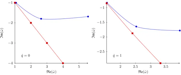
Figure 1. The first few QNM frequencies, divided by 2πT, of the electromagnetic current operator for ˆq= 0 (left) and ˆq= 1 (right), evaluated at λ=∞ (red squares) andλ= 1000 (blue circles).
Theλ= 1000 results include the O(γ) corrections, but no higher order contributions. Lines have been inserted merely to guide the eye.
while the resultingγ-corrected effective potential reads V(u) = −u+ ˆω2−qˆ2f(u)
uf(u)2
+ γ
144f(u)
h−11700 + 2098482u2−4752055u4+ 1838319u6 + ˆq2 4770u−1+ 11700u−953781u3+ 1011173u5
−ωˆ2 4770u−1+ 28170u−1199223u3i
. (3.16)
Given the above potential, solutions to the equation Ψ00 = V Ψ may be expanded in a power series in γ. The black brane horizon at u = 1 is a regular singular point of the equation, where infalling solutions behave locally as Ψ(u) ∼ (1−u)r with characteristic exponentr = 12(1−iˆω). Hence, one may expand the solutions of interest as
Ψ(u) = (1−u)rh
Φ(0)(u) +γΦ(1)(u) +· · ·i
, (3.17)
where Φ(0) and Φ(1) have the near-horizon Frobenius expansions, Φ(0)(u)∼
∞
X
n=0
an(1−u)n, Φ(1)(u)∼
∞
X
n=0
bn(1−u)n. (3.18) One may further determine the coefficients {an} and {bn} recursively by inserting these expansions into eq. (3.6) and collecting like powers of γ and (1−u). Without loss of generality, one may set a0 = 1 and b0= 0.
The values of frequency, for which the solution also satisfies the Dirichlet condition at the boundary (for a fixedq), may also be expanded in powers of γ,
ˆ
ω= ˆω(0)+γωˆ(1)+· · · . (3.19)
JHEP11(2015)087
If the expansion (3.18) is truncated at some upper limitN and used throughout the com- putational domain 0 ≤ u ≤ 1, then the Dirichlet condition that Ψ(0) vanish (for all γ) reduces to a set of algebraic equations
N
X
n=0
an(ˆω(0)) = 0,
N
X
n=0
bn(ˆω(0),ωˆ(1)) = 0, (3.20) whose roots yield (approximations to) ˆω(0)and ˆω(1). Carrying out this procedure for values of N sufficiently large that the results are stable turns out to be a viable computational strategy [51]. Our results for the first few QNMs are displayed in figure 1and reported in table 2 below, and fully agree with the findings of ref. [51].
We have also computed the photoemission spectrum (3.11) by solving the γ-corrected equation for the transverse electric field, as in ref. [46], and then evaluated the first few moments (2.2) of the spectrum, obtaining the results shown in table 1.
As an alternative to the above approach, in which the QNM frequencies and mode functions are explicitly expanded in powers of γ, one may directly solve the Schrodinger equation (3.6) with the potential (3.16) evaluated at some chosen value of γ. Spectral methods provide an efficient numerical approach [58]. We write
Ψ(u) = (1−u)rΦ(u), (3.21)
so that the function Φ(u) is regular at both the horizon and boundary. In terms of Φ, the explicit γ-corrected QNM equation takes the form
−u(1+u)(1−u2) Φ00(u) +u(1+u)2(1−iˆω) Φ0(u) +K(u) Φ(u) = 0, (3.22) with
K(u)≡(1−ωˆ2) +1
4u(1−3ˆω2)−1
4u2(1 + ˆω2) + γ
144(1+u)h
11700u+ 2098482u3−4752055u5+ 1838319u7 + ˆq2 4770 + 11700u2−953781u4+ 1011173u6 + ˆω2 −4770−28170u2+ 1199223u4i
. (3.23)
Next, we expand Φ in a truncated series of Chebyshev polynomials, Φ(u) =
N
X
n=0
cnTn(2u−1), (3.24)
withTn(z)≡cos(ncos−1z).4 Requiring equation (3.22) to be satisfied at the pointsuj ≡
1
2[1−cos(jπ/N)],j = 0,1,· · ·N, which comprise a Chebyshev-Gauss-Lobatto grid, converts the differential equation (3.22) into a finite matrix equation of the formA·v= 0. Here,vis a vector consisting of theN+1 coefficients{cn}of the Chebyshev expansion, whileAdenotes
4The Chebyshev polynomials{Tn(z)}form an orthogonal basis in the Hilbert space with inner product (f, g) =R1
−1dz f(z)g(z)/√ 1−z2.
JHEP11(2015)087
ˆ q= 0
1 2 3 4 5
−4
−3
−2
−1
Re(ˆω)
Im(ˆω)
ˆ q= 1
2 2.5 3 3.5
−2.5
−2
−1.5
−1
Re(ˆω)
Im(ˆω)
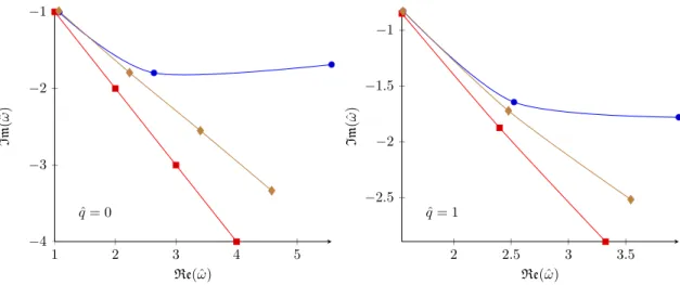
Figure 2. The first few QNM frequencies, divided by 2πT, of the electromagnetic current operator for ˆq= 0 (left figure) or ˆq= 1 (right figure) atλ= 1000. Results obtained by directly solving the QNM equation at this value of λusing spectral methods are shown as brown diamonds, while the red squares and blue circles show the same zeroth and first order results, respectively, previously displayed in figure1. Again, lines merely serve to guide the eye.
ˆ
ωEMk (ˆq= 0) ωˆEMk (ˆq= 1)
k O(γ0) O(γ1) resummed O(γ0) O(γ1) resummed
1 1−i 1.073−1.005i 1.068−0.990i 1.547−0.85i 1.558−0.828i 1.557−0.829i 2 2−2i 2.637−1.797i 2.237−1.794i 2.399−1.874i 2.525−1.645i 2.477−1.722i 3 3−3i 5.536−1.692i 3.403−2.551i 3.323−2.859i 3.957−1.791i 3.544−2.518i 4 4−4i 11.07 + 0.47i 4.57−3.34i 4.28−3.91i 6.37−0.39i 4.67−3.31i Table 2. The first four QNM frequencies, divided by 2πT, of the electromagnetic current operator {ωˆEMk }, k= 1,· · ·4, for ˆq= 0 (left) and ˆq= 1 (right), atλ= 1000. Respective columns show the results from the zeroth order, first order, and resummed approximations discussed in the text.
a matrix whose entries on the j’th row are obtained by evaluating eq. (3.22) at the j’th grid point.5 Nonvanishing solutions of this homogeneous set of equations only exist when
det(A) = 0. (3.25)
This determinant is a polynomial in ˆω, whose roots {ωˆ(Nk )} rapidly converge (for fixed k) as the number of grid points N increases. Evaluating these roots numerically is straight- forward (for relatively modest values of N) given specific values of the wavevector ˆq and the parameterγ.
Solving the QNM equation in the fashion described above yields values for the quasi- normal mode frequencies with nonlinear dependence on γ. One has, in effect, resummed a subset of higher order contributions to the QNM frequencies which arise solely from the
5The row of this matrix corresponding to the u = 0 endpoint automatically enforces the Dirichlet boundary condition Φ(0) = 0.
JHEP11(2015)087
λbreakdown(ˆq= 0) λbreakdown(ˆq= 1) k O(γ1) resummed O(γ1) resummed
1 139 ≈22.5 57.1 <5
2 382.2 ≈21.7 195 ≈8
3 767.5 ≈21.3 437 ≈14
4 1298 ≈21.1 793 ≈16
Table 3. Values of λbelow which the deviation of the QNM frequencyωkEMfrom itsλ=∞limit exceeds theλ=∞value. Respective columns show the results obtained using either the first order or resummed approximations for the QNM frequency.
first order, i.e. O(γ), correction to the supergravity action. One may hope — although there is no guarantee — that this is the dominant source of all higher order contributions.
In figure2and table2, we display the effects of the resummation for the first few QNM frequencies, again at λ= 1000 and both ˆq = 0 and ˆq = 1, and compare the results to the previous unresummed values. As can be readily verified, the size of the O(γ) correction increases rapidly with the QNM mode number k, asymptotically growing like k4. This reflects the fact that finite coupling corrections arise from higher dimension operators in the supergravity action (3.14). Although the size of the O(γ) correction to the first QNM frequency appears modest atλ= 1000, as seen in the top row of table2, theO(γ) correction exceeds the leading λ =∞ value of the first QNM frequency at λ = 139 (for q = 0), or λ= 57.1 (forq = 1), above our benchmark phenomenological range. For the second mode (as noted previously) and all higher modes, the “breakdown” values ofλ, below which the O(γ) correction exceeds the leading term, are even larger.
In contrast, our resummed approximation for the QNM frequencies yields results which deviate from the λ= ∞ values substantially less. As a concrete measure of this, table 3 compares, for the first few modes, the breakdown values of λbelow which the deviation of the QNM frequency from its λ = ∞ value exceeds the λ = ∞ result, in either scheme.6 For the resummed approximation, we find that these nominal breakdown values of λ are substantially smaller than the breakdown values of the first order results. For the first four modes, the breakdown values of the resummed approximation lie within or below our benchmark phenomenological range of 10–40. Moreover, the breakdown values of the resummed approximation grow far less rapidly with mode number than do theO(γ) results.
One may also apply our partial resummation scheme when evaluating the zero- frequency slope of the correlator which determines the electric conductivity of the N = 4 SYM plasma via eq. (3.10). However, since the conductivity receives a much smallerO(γ) correction than do the QNM frequencies, the effect of the resummation is much more mod- est for the conductivity. At, for example, λ= 1000 the relative size of the O(γ) correction to the conductivity is about 8×10⁻³, and our resummation increases this deviation from
6When computing resummed approximations, the convergence of both the Frobenius (3.18) and spec- tral (3.24) expansions progressively degrade as the value ofγ is increased, making precise determinations of breakdown values ofλchallenging.
JHEP11(2015)087
the λ=∞ value by a further 5×10⁻⁵. In contrast to the situation with QNM frequen- cies, the nominal breakdown value of the resummed approximation for the conductivity is somewhat larger than the breakdown value of the first order approximation (λ≈ 57.9 instead of 39.7).
3.2 Stress-energy correlator
The dynamics of linearized metric perturbations determine the stress-energy tensor corre- lator. We will focus on the ` = 2 or shear channel, for which it is sufficient to consider δgxy as the only non-zero component of the perturbation when the wavevector points in thez-direction.7 After Fourier transforming with respect to the boundary coordinates, the rescaled perturbation
Z(u)≡ u
r2hδgxy(u) (3.26)
satisfies theO(γ) corrected equation of motion [59],
−Z00(u) +P(u)Z0(u) +Q(u)Z(u) = 0, (3.27) with
P(u)≡ 1 +u2 uf(u) +1
4γ 600u−2306u3−3171u5−3840 ˆq2u4
(3.28) and
Q(u)≡ −(1 + 30γ)ωˆ2−qˆ2f(u) uf(u)2
− γ 4f(u)2
h
50u2−275u6+ 225u8
+ ˆω2 600u−2856u3+ 2136u5
+ ˆq2 −300u+ 3456u3−6560u5+ 3404u7 + ˆq4 768u4+ 768u6i
. (3.29)
Boundary conditions for finding quasinormal modes are the same as discussed earlier:
infalling behavior at the horizon and Dirichlet at the boundary. Solutions up toO(γ) of the above equation were found in ref. [50] using the Frobenius expansion technique discussed in the previous subsection. One may, however, also solve the equation directly for specific values ofγ, just as we did for the electromagnetic current correlator, using spectral methods.
Figure3shows a comparison of the results of the two approaches forλ= 500 and ˆq= 0, with table 4 listing explicit values. Once again, at this value of λ(which is still well above the phenomenologically relevant range) we observe a substantial difference between the O(γ) results and our resummed values, with the resummation decreasing the difference from the
7Note that in ref. [57], the channel with`= 2 rotational symmetry about the wavevector was referred to as the “scalar channel” because the corresponding metric perturbation satisfies the same equation as a minimally coupled massless scalar, and the`= 1 or vector channel was referred to as the “shear channel”.
Our terminology is motivated by the fact that the shear viscosity can be obtained from the zero-frequency limit of the correlator in the`= 2 channel.
JHEP11(2015)087
ˆ q= 0
2 3 4 5
−4
−3
−2
Re(ˆω)
Im(ˆω)
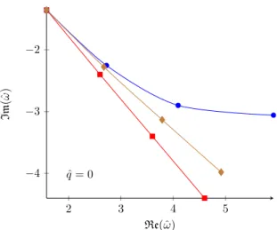
Figure 3. The first few QNM frequencies, divided by 2πT, for the shear channel of the stress- energy correlator, evaluated for ˆq= 0 and λ= 500. Results obtained by directly solving the QNM equation at this value of λ using spectral methods are shown as brown diamonds, while the red squares and blue circles show results truncated at zeroth and first order in γ, respectively. As before, lines merely serve to guide the eye.
ˆ
ωsheark (ˆq = 0)
k O(γ0) O(γ1) resummed
1 1.560−1.373i 1.581−1.356i 1.579−1.356i 2 2.585−2.382i 2.723−2.253i 2.673−2.277i 3 3.594−3.385i 4.093−2.899i 3.789−3.133i 4 4.60−4.39i 5.92−3.07i 4.91−3.98i
Table 4. The first four QNM frequencies, divided by 2πT, {ωˆsheark }, k = 1,· · ·4, in the shear channel of the stress-energy correlator, for ˆq= 0 andλ= 500. Respective columns show the results from the zeroth order, first order, and resummed approximations discussed in the text.
λbreakdown k O(γ1) resummed 1 27.6 <1 2 71.2 <1 3 135.5 <1 4 221 <1
Table 5. Values ofλbelow which the deviation of the QNM frequencyωsheark from itsλ=∞limit exceeds theλ=∞value. Respective columns show the results obtained using either the first order or resummed approximations for the QNM frequency.
JHEP11(2015)087
λ=∞ limit. In parallel with the previous subsection, we show in table 5 the breakdown values of λ, computed with both first order and resummed approximations, below which the first few shear channel QNM frequencies deviate from their λ = ∞ limits by more than theirλ=∞ values. We find that for the shear channel quasinormal frequencies, our resummation scheme leads to nominal breakdown values of λ for all modes up to k = 4 lying below our benchmark phenomenological range of 10–40.
Similarly to the plasma conductivity considered earlier, the shear viscosity is deter- mined by the zero-frequency slope of the retarded correlator of Txy evaluated at vanishing wavenumber,
η=−lim
ω→0 Im1
ωGretxy,xy(ω,0). (3.30)
IncludingO(γ) corrections, it can be shown that this correlator is given by [43]
Gretxy,xy(ω, q) = lim
u→0
Nc2(rh0)4 4π2
Z0(u)
u Z(u), (3.31)
where Z(u) is a solution to eqs. (3.27)–(3.29) at ˆq = 0 that satisfies infalling boundary conditions at the horizon, and rh0 =πT L2/(1 + 15γ) is the horizon position of the γ = 0 geometry.8 Using the Frobenius method to solve for the metric perturbation to linear order inγ now leads to
Gretxy,xy(ω,0) =−iNc2(rh0)4ω
8π3T (1 + 195γ) +O(ω2, γ2), (3.32) from which one can extract the result found in ref. [44],η = π8 Nc2T3(1 + 135γ+· · ·).
One may also apply our partial resummation scheme when evaluating the zero- frequency slope of the correlator (3.31). As with the conductivity, since the shear viscosity receives a much smaller O(γ) correction than do the QNM frequencies, the effect of the resummation is much more modest for the this transport coefficient. At, for example, λ= 1000 the relative size of theO(γ) correction to the viscosity is about 6×10⁻⁴, and our resum- mation increases this deviation from theλ=∞value by a mere 10−7. As with conductivity, the resummed approximation for the shear viscosity leads to a somewhat larger nominal breakdown value ofλas compared to the first order approximation (λ≈14 instead of≈7).
4 Conclusions
Our examination of finite-λcorrections to holographic results for thermal quantities is moti- vated by an obvious desire to understand more clearly the applicability of gauge/gravity du- ality to the physics of quark-gluon plasma as produced in real heavy ion collisions. In partic- ular, how large an error is made when the system is modeled as infinitely strongly coupled, as is customary in most holographic calculations of non-equilibrium dynamics performed in the supergravity limit? We approached this problem by comparing the behaviors of the strong coupling expansions for a variety of thermal quantities, for which the leading order
8This γ = 0 horizon position, used consistently in ref. [43], differs from the horizon position rh = πT L2/(1 +26516 γ) of theγ-corrected metric derived in ref. [60] and used throughout refs. [19,45,46].
JHEP11(2015)087
finite coupling correction, of order λ−3/2 in the ’t Hooft coupling, is known. Our compari- son has singled out quasinormal mode frequencies as quantities for which the finite coupling corrections appear particularly problematic at phenomenologically interesting values of the
’t Hooft coupling. We discovered, however, that a partial inclusion of higher order contribu- tions, generated by the leading corrections to the supergravity action, leads to a dramatic reduction in the predicted size of finite coupling effects in quasinormal mode frequencies.
One clear, but unsurprising, message of our comparison is that notions of strong (or weak) coupling domains can depend rather strongly on the physics observable of interest.
For some quantities, ’t Hooft couplings of order 10–40 may be easily accessible via a one or two term strong coupling expansion, while for other quantities this is clearly not the case.
The full reasons underlying such behavior are unclear, but some insight may perhaps be drawn from similar issues at weak coupling. There, an extensive amount of work has been devoted to the calculation of high order perturbative results for a number of equilibrium thermodynamic quantities. An important lesson from this work is that the convergence of perturbation theory is intimately related to the relative influence of different momentum or energy scales contributing to the observable in question. Weak coupling expansions for physical quantities that are dominantly sensitive to the hard thermal scale of 2πT are found to behave significantly better than expansions of quantities which are more sensitive to the soft gT and ultrasoft g2T scales which originate from electro- and magnetostatic screening, respectively. The degraded perturbative stability arises from the dependence on the ratio of these scales, which appears in the form of contributions suppressed only by single powers (and logarithms) of g, instead of αs =g2/(4π). Ultimately, this reflects the diverging infrared sensitivity of the Bose-Einstein distribution of gluonic fields.
Whether it is possible to interpret differences in stability of strong coupling expan- sions in an analogous manner remains to be seen. However, considering the fact that the O(α03) corrections toλ=∞results originate from higher derivative operators added to the supergravity action, and that the leading finite coupling corrections to the QNM frequen- cies can be seen to grow rapidly with the mode number, perhaps such expectations are not completely unfounded. In the meantime, trying to generalize many more holographic calcu- lations to include at least the leading finite ’t Hooft couplings would clearly be worthwhile.
Acknowledgments
The authors would like to thank Andreas Karch, Andrei Starinets, and Stefan Stricker for useful discussions. The work of A.V. was supported by the Academy of Finland, grant Nr.
273545. The work of L.Y. was supported, in part, by the U.S. Department of Energy under Grant No. DE-SC0011637, and by the Alexander von Humboldt Foundation. L.Y. thanks the University of Regensburg and the Alexander von Humboldt Foundation for generous support and hospitality during portions of this work. A.V. and S.W. thank the Institute for Nuclear Theory at the University of Washington for its hospitality and support during the completion of this work.
Open Access. This article is distributed under the terms of the Creative Commons Attribution License (CC-BY 4.0), which permits any use, distribution and reproduction in any medium, provided the original author(s) and source are credited.
JHEP11(2015)087
References
[1] E.V. Shuryak,What RHIC experiments and theory tell us about properties of quark-gluon plasma?,Nucl. Phys. A 750(2005) 64 [hep-ph/0405066] [INSPIRE].
[2] N. Brambilla et al.,QCD and strongly coupled gauge theories: challenges and perspectives, Eur. Phys. J.C 74(2014) 2981[arXiv:1404.3723] [INSPIRE].
[3] C. Gale, S. Jeon and B. Schenke,Hydrodynamic modeling of heavy-ion collisions,Int. J.
Mod. Phys.A 28(2013) 1340011[arXiv:1301.5893] [INSPIRE].
[4] P. Kovtun, D.T. Son and A.O. Starinets,Viscosity in strongly interacting quantum field theories from black hole physics, Phys. Rev. Lett.94 (2005) 111601[hep-th/0405231]
[INSPIRE].
[5] E. Laermann and O. Philipsen,The status of lattice QCD at finite temperature,Ann. Rev.
Nucl. Part. Sci.53(2003) 163[hep-ph/0303042] [INSPIRE].
[6] S.S. Gubser and A. Karch,From gauge-string duality to strong interactions: a pedestrian’s guide,Ann. Rev. Nucl. Part. Sci.59(2009) 145[arXiv:0901.0935] [INSPIRE].
[7] J. Casalderrey-Solana, H. Liu, D. Mateos, K. Rajagopal and U.A. Wiedemann,Gauge/string duality, hot QCD and heavy ion collisions,arXiv:1101.0618[INSPIRE].
[8] P.M. Chesler and W. van der Schee,Early thermalization, hydrodynamics and energy loss in AdS/CFT,arXiv:1501.04952[INSPIRE].
[9] C.P. Herzog, A. Karch, P. Kovtun, C. Kozcaz and L.G. Yaffe,Energy loss of a heavy quark moving throughN = 4 supersymmetric Yang-Mills plasma,JHEP 07(2006) 013
[hep-th/0605158] [INSPIRE].
[10] E. Caceres and A. Guijosa,On drag forces and jet quenching in strongly coupled plasmas, JHEP 12 (2006) 068[hep-th/0606134] [INSPIRE].
[11] E. Caceres and A. Guijosa,Drag force in charged N = 4SYM plasma, JHEP 11(2006) 077 [hep-th/0605235] [INSPIRE].
[12] S.S. Gubser,Drag force in AdS/CFT,Phys. Rev.D 74(2006) 126005 [hep-th/0605182]
[INSPIRE].
[13] J. Casalderrey-Solana and D. Teaney, Transverse momentum broadening of a fast quark in a N= 4 Yang-Mills plasma,JHEP 04(2007) 039[hep-th/0701123] [INSPIRE].
[14] P.M. Chesler, K. Jensen, A. Karch and L.G. Yaffe,Light quark energy loss in
strongly-coupledN = 4supersymmetric Yang-Mills plasma,Phys. Rev. D 79(2009) 125015 [arXiv:0810.1985] [INSPIRE].
[15] S.S. Gubser, D.R. Gulotta, S.S. Pufu and F.D. Rocha, Gluon energy loss in the gauge-string duality,JHEP 10 (2008) 052[arXiv:0803.1470] [INSPIRE].
[16] P.M. Chesler, K. Jensen and A. Karch,Jets in strongly-coupled N = 4super Yang-Mills theory,Phys. Rev.D 79(2009) 025021 [arXiv:0804.3110] [INSPIRE].
[17] P.M. Chesler and K. Rajagopal,Jet quenching in strongly coupled plasma,Phys. Rev.D 90 (2014) 025033[arXiv:1402.6756] [INSPIRE].
[18] S. Caron-Huot, P. Kovtun, G.D. Moore, A. Starinets and L.G. Yaffe, Photon and dilepton production in supersymmetric Yang-Mills plasma,JHEP 12 (2006) 015[hep-th/0607237]
[INSPIRE].
JHEP11(2015)087
[19] B. Hassanain and M. Schvellinger, Plasma photoemission from string theory,JHEP 12 (2012) 095[arXiv:1209.0427] [INSPIRE].
[20] R. Baier, S.A. Stricker, O. Taanila and A. Vuorinen, Holographic dilepton production in a thermalizing plasma,JHEP 07(2012) 094[arXiv:1205.2998] [INSPIRE].
[21] R. Baier, S.A. Stricker, O. Taanila and A. Vuorinen, Production of prompt photons:
holographic duality and thermalization, Phys. Rev.D 86(2012) 081901[arXiv:1207.1116]
[INSPIRE].
[22] B. M¨uller and D.-L. Yang, Production of prompt photons and dileptons in rapid holographic thermalization,arXiv:1212.3354[INSPIRE].
[23] P.M. Chesler and L.G. Yaffe,Horizon formation and far-from-equilibrium isotropization in supersymmetric Yang-Mills plasma,Phys. Rev. Lett.102(2009) 211601 [arXiv:0812.2053]
[INSPIRE].
[24] M.P. Heller, D. Mateos, W. van der Schee and D. Trancanelli, Strong coupling isotropization of non-Abelian plasmas simplified,Phys. Rev. Lett.108(2012) 191601[arXiv:1202.0981]
[INSPIRE].
[25] M.P. Heller, D. Mateos, W. van der Schee and M. Triana, Holographic isotropization linearized,JHEP 09(2013) 026[arXiv:1304.5172] [INSPIRE].
[26] J.F. Fuini and L.G. Yaffe,Far-from-equilibrium dynamics of a strongly coupled non-Abelian plasma with non-zero charge density or external magnetic field,JHEP 07(2015) 116 [arXiv:1503.07148] [INSPIRE].
[27] P.M. Chesler and L.G. Yaffe,Boost invariant flow, black hole formation and
far-from-equilibrium dynamics inN = 4 supersymmetric Yang-Mills theory, Phys. Rev.D 82 (2010) 026006[arXiv:0906.4426] [INSPIRE].
[28] M.P. Heller, R.A. Janik and P. Witaszczyk, The characteristics of thermalization of boost-invariant plasma from holography,Phys. Rev. Lett.108(2012) 201602
[arXiv:1103.3452] [INSPIRE].
[29] H. Bantilan, F. Pretorius and S.S. Gubser, Simulation of asymptotically AdS5 spacetimes with a generalized harmonic evolution scheme,Phys. Rev. D 85(2012) 084038
[arXiv:1201.2132] [INSPIRE].
[30] H. Bantilan and P. Romatschke, Simulation of black hole collisions in asymptotically anti-de Sitter spacetimes,Phys. Rev. Lett.114(2015) 081601[arXiv:1410.4799] [INSPIRE].
[31] B. Wu,On holographic thermalization and gravitational collapse of tachyonic scalar fields, JHEP 04 (2013) 044[arXiv:1301.3796] [INSPIRE].
[32] U.H. Danielsson, E. Keski-Vakkuri and M. Kruczenski,Spherically collapsing matter in AdS, holography and shellons,Nucl. Phys.B 563(1999) 279[hep-th/9905227] [INSPIRE].
[33] O. Taanila,Holographic thermalization and Oppenheimer-Snyder collapse, arXiv:1507.00878[INSPIRE].
[34] P.M. Chesler and L.G. Yaffe,Holography and colliding gravitational shock waves in asymptotically AdS5 spacetime,Phys. Rev. Lett.106(2011) 021601[arXiv:1011.3562]
[INSPIRE].