doi: 10.3389/fmars.2019.00061
Edited by:
Marius Nils Müller, Federal University of Pernambuco, Brazil
Reviewed by:
Soultana Zervoudaki, Hellenic Centre for Marine Research (HCMR), Greece Jun Sun, Tianjin University of Science and Technology, China
*Correspondence:
María Algueró-Muñiz maria.alguero@awi.de
†These authors have contributed equally to this work
Specialty section:
This article was submitted to Marine Biogeochemistry, a section of the journal Frontiers in Marine Science
Received:28 March 2018 Accepted:05 February 2019 Published:25 February 2019
Citation:
Algueró-Muñiz M, Horn HG, Alvarez-Fernandez S, Spisla C, Aberle N, Bach LT, Guan W, Achterberg EP, Riebesell U and Boersma M (2019) Analyzing the Impacts of Elevated-CO2Levels on the Development of a Subtropical Zooplankton Community During Oligotrophic Conditions and Simulated Upwelling.
Front. Mar. Sci. 6:61.
doi: 10.3389/fmars.2019.00061
Analyzing the Impacts of Elevated-CO 2 Levels on the Development of a Subtropical Zooplankton Community During Oligotrophic Conditions and
Simulated Upwelling
María Algueró-Muñiz1*†, Henriette G. Horn1,2†, Santiago Alvarez-Fernandez1, Carsten Spisla1,3, Nicole Aberle1,4, Lennart T. Bach3, Wanchun Guan5, Eric P. Achterberg3, Ulf Riebesell3and Maarten Boersma1,6
1Biologische Anstalt Helgoland, Alfred-Wegener-Institut Helmholtz-Zentrum für Polar- und Meeresforschung, Bremerhaven, Germany,2Department of Estuarine and Delta Systems, NIOZ Royal Netherlands Institute for Sea Research and Utrecht University, Yerseke, Netherlands,3GEOMAR Helmholtz Centre for Ocean Research Kiel, Kiel, Germany,4Department of Biology, Trondheim Biological Station, Norwegian University of Science and Technology, Trondheim, Norway,
5Department of Marine Biotechnology, School of Laboratory Medicine and Life Science, Wenzhou Medical University, Wenzhou, China,6Department of Biology/Chemistry, University of Bremen, Bremen, Germany
Ocean acidification (OA) is affecting marine ecosystems through changes in carbonate chemistry that may influence consumers of phytoplankton, often via trophic pathways.
Using a mesocosm approach, we investigated OA effects on a subtropical zooplankton community during oligotrophic, bloom, and post-bloom phases under a range of different pCO2 levels (from ∼400 to ∼1480 µatm). Furthermore, we simulated an upwelling event by adding 650 m-depth nutrient-rich water to the mesocosms, which initiated a phytoplankton bloom. No effects of pCO2 on the zooplankton community were visible in the oligotrophic conditions before the bloom. The zooplankton community responded to phytoplankton bloom by increased abundances in all treatments, although the response was delayed under high-pCO2 conditions. Microzooplankton was dominated by small dinoflagellates and aloricate ciliates, which were more abundant under medium- to high-pCO2conditions. The most abundant mesozooplankters were calanoid copepods, which did not respond to CO2 treatments during the oligotrophic phase of the experiment but were found in higher abundance under medium- and high-pCO2 conditions toward the end of the experiment, most likely as a response to increased phyto- and microzooplankton standing stocks. The second most abundant mesozooplankton taxon were appendicularians, which did not show a response to the different pCO2 treatments. Overall, CO2 effects on zooplankton seemed to be primarily transmitted through significant CO2 effects on phytoplankton and therefore indirect pathways. We conclude that elevated pCO2 can change trophic cascades with significant effects on zooplankton, what might ultimately affect higher trophic levels in the future.
Keywords: microzooplankton, mesozooplankton, mesocosms, ocean acidification, nutrients,Oncaea, trophic transfer efficiency
INTRODUCTION
Anthropogenic emissions are increasing atmospheric CO2
concentrations from pre-industrial levels of ∼280 µatm to current levels of over 400µatm, and increases up to 1000µatm by the end of the century are projected for the RCP8.5 emission scenario (IPCC, 2013). The oceans act as carbon sinks, absorbing about one third of the anthropogenic CO2 emission (Sabine et al., 2004). This oceanic CO2uptake causes a shift in carbonate chemistry with a decrease in seawater pH, commonly known as ocean acidification (OA). Recent years of intense research have shown that OA may cause substantial changes to marine ecosystems (IPCC, 2013;Kroeker et al., 2013).
Despite the large body of literature related to biological responses to OA, most studies investigated single species responses, which may rarely provide a sufficient basis to understand long-term responses in complex ecological environments (Harley, 2011; Queirós et al., 2015). Moreover, changes inpCO2may promote changes in trophic interactions, leading to the dampening or amplification of single species effects and hence promoting shifts in community composition (Lischka et al., 2011; Rossoll et al., 2012, 2013). Consequently, in situcommunity studies are important in order to evaluate OA effects at the level of assemblages and ecosystems (Guinotte and Fabry, 2008;Riebesell and Gattuso, 2015).
Focusing on marine plankton, nutrient conditions can determine how communities respond to OA (Alvarez-Fernandez et al., 2018), being the most noticeable pCO2 effects often observed under limiting inorganic nutrient conditions (Paul et al., 2015;Sala et al., 2015;Bach et al., 2016b). This is because elevated CO2levels cause an increase in phytoplankton standing stocks —more pronounced in smaller-sized taxa— and this effect on primary producers may be transferred differently into heterotroph primary consumers depending on the inorganic nutrient availability (Alvarez-Fernandez et al., 2018). The present study focussed on an oligotrophic system around the island of Gran Canaria within the Canary Archipelago, located in the subtropical North Atlantic Ocean. Despite its overall oligotrophic character, this region experiences a short-term period of deep-water nutrient inputs in later winter (February–
March) (de León and Braun, 1973; Cianca et al., 2007) as well as recurrent mesoscale upwelling events that act as an offshore pump of organic matter and carbon (Sangrà et al., 2009). The so-calledlate winter bloomusually causes an increase in primary production and chlorophyll a concentration in the euphotic zone (Menzel and Ryther, 1961; Arístegui et al., 2001). Typically, mesozooplankton grazing pressure exerted on phytoplankton is low in the study area (Arístegui et al., 2001;Hernández-León et al., 2004), and mesozooplankters are considered to feed on microzooplankton which, in turn, control primary production (Hernández-León et al., 2001;Quevedo and Anadón, 2001;Calbet and Alcaraz, 2007). The microzooplankton community is usually dominated by small dinoflagellates and aloricate ciliates (Quevedo and Anadón, 2001), while the most important mesozooplankton during the annual cycle are copepods (Hernández-León et al., 2007). However, the plankton community typically changes during bloom conditions
(Arístegui et al., 2001; Hernández-León et al., 2004; Schmoker et al., 2012). An increase in copepod abundances follows the increase in primary production, and a trophic cascade caused by the consumption of microzooplankton by mesozooplankton allows a further increase in autotrophic biomass by the combined effect of top-down control and nutrient remineralization (Hernández-León, 2009; Schmoker et al., 2012). This bloom situation may cause a reduction in the efficiency of the food web, considering that trophic transfer efficiency (i.e., zooplankton growth per unit phytoplankton production) tends to be diminished under nutrient enrichment conditions due to the limited capacity of grazers to use the boosted algae production (Calbet et al., 1996;Kemp et al., 2001;Calbet et al., 2014).
In order to assess the impacts of OA on zooplankton communities we must consider not only direct effects on zooplankton caused by pH reductions, but also effects that reach consumers indirectly, through trophic pathways (Boersma et al., 2008; Rossoll et al., 2012; Cripps et al., 2016). Detrimental indirect pCO2 effects have been described in single species of herbivores (Schoo et al., 2013; Meunier et al., 2016) and secondary consumers (Lesniowski et al., 2015). In the case of copepods, bottom-up influences of OA seem to be largely associated with interspecific differences among prey items with regard to their sensitivity to elevated pCO2 levels, as observed when analyzing the cellular stoichiometry of copepods’
photosynthetic preys (Isari et al., 2015; Meunier et al., 2016).
In turn, microzooplankton may be affected by the effect of high pCO2levels on phytoplankton availability or quality such as an increase in picophytoplankton standing stock or changes in their cellular carbon-to-nutrient ratios (Bach et al., 2016b; Meunier et al., 2016). In addition, a high pCO2 scenario is likely to favor harmful algal blooms (Wells et al., 2015) with substantial consequences for energy transfer from primary producers to consumers within marine communities.
Plankton community OA studies to date have been mostly carried out in relatively eutrophic environments (but see Sala et al., 2015;Gazeau et al., 2017), and led to varying conclusions.
Some studies showed the lack of major effects of elevated pCO2 levels in micro- (Aberle et al., 2013; Horn et al., 2016) and mesozooplankton abundances (Niehoff et al., 2013), while others detected both changes in community size distributions and biomass (Lischka et al., 2017; Taucher et al., 2017b) as well as positive bottom-uppCO2responses on mesozooplankton abundances (Algueró-Muñiz et al., 2017). Inorganic nutrient availability can control these different responses to OA in planktonic communities, thereby the nutrient-deplete phases could determine the transfer of the pCO2 effects on primary producers to primary consumers (Alvarez-Fernandez et al., 2018). Taking this into account, studying OA effect in oligotrophic systems —which represent most of the global surface ocean— becomes of paramount importance. To accomplish this goal, we performed an experiment that allowed us to study the contrast between nutrient-depleted and nutrient-replete periods.
Our aim was to analyze the effects of OA on the development of an autumn zooplankton community from the subtropical North Atlantic, including a simulated bloom situation. We assessed the effects ofpCO2on (1) the abundance of subtropical
micro- and mesozooplankton under oligotrophic and upwelling conditions, (2) the size and reproductive output of an important copepod species and (3) the trophic efficiency within the plankton community under different conditions.
MATERIALS AND METHODS Mesocosms Setup and Experimental Design
The experiment was conducted from 27th September (t-4) until 26th November 2014 (t56) within the framework of the BIOACID II project (Biological Impacts of Ocean ACIDification) and was hosted by the Plataforma Oceánica de Canarias (PLOCAN, Spain). In order to study the effects of changing carbonate chemistry conditions on the plankton community succession, nine mesocosms (KOSMOS, M1–M9: “Kiel Off-Shore Mesocosms for Ocean Simulation”), were deployed in Gando Bay (27◦5504100 N, 15◦2105500 W), on the west coast of Gran Canaria (Canary Islands, Spain) (Taucher et al., 2017a). The nine cylindrical mesocosm units (13 m deep, 2 m diameter) enclosed water volumes (∼35 m3) sealed by sediment traps installed at the bottom of each mesocosm bag (Boxhammer et al., 2016).
Target pCO2 was reached at the beginning of the experiment by adding CO2 saturated seawater to the mesocosms following the protocol described inRiebesell et al. (2013). The carbonate
chemistry of the enclosed seawater was manipulated by stepwise additions of CO2-saturated seawater in four steps over 7 days.
Two further CO2 additions were conducted on days 21 and 38 to compensate for the loss of CO2through air-sea gas exchange.
AspCO2treatments we established a gradient from current levels to end-of-century scenarios, representing IPCC predictions for mitigation scenarios (RCP 2.6) as well as medium (RCP 6.0) and high (RCP 8.5)pCO2levels (IPCC, 2013). The meanpCO2
values per mesocosms between t1 and t55 were M1 = 369, M2 = 887, M3 = 563, M4 = 716, M5 = 448, M7 = 668, M8 = 1025 and M9 = 352 µatm. Analyzing the oligotrophic phase of the experiment, we could differentiate three pCO2 groups by a k-means cluster analysis (Jain, 2010). The outcome showed three distinguishable clusters: low-pCO2(M1, M9, M5;k= 460µatm) medium-pCO2 (M3, M7, M4; k= 721 µatm) and high-pCO2
levels (M2, M8;k= 1111µatm) (Figure 1A) which were used for the analyses presented throughout this paper. Unfortunately, we detected a hole in the enclosure bag of the third high-pCO2 mesocosm (M6 = 976 µatm) on t27, so M6 was excluded from sampling and analyses after that date.
To simulate a natural upwelling event, we collected deep water (∼84 m3) from 650 m depth on t22, as described byTaucher et al.
(2017a). From each mesocosm, a defined volume of water was removed from 5 m depth with a submersible pump (Grundfos SP-17-5R). Consequently, in a process of∼9 h duration during the night of t24, deep water was pumped into the mesocosms,
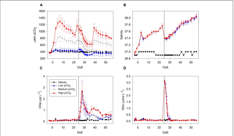
FIGURE 1 |Development of core parameters throughout the experiment.(A)pCO2(µatm),(B)salinity,(C)Chla(µg L−1),(D)NOx (nitrate+nitrite;µmol L−1). The addition of deep water (DW) in the mesocosms took place during the night between the 24th and 25th day of experiment (DoE); dashed line. Note that a clear draw down of CO2occurred during the phytoplankton bloom (t25–t35). Color code: black = Atlantic, blue = low-pCO2, gray = medium-pCO2, red = high-pCO2.
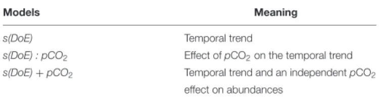
TABLE 1 |Generalized additive mixed model (GAMM) structures.
Models Meaning
s(DoE) Temporal trend
s(DoE) : pCO2 Effect ofpCO2on the temporal trend s(DoE)+pCO2 Temporal trend and an independentpCO2
effect on abundances DoE, day of experiment.
reaching a mixing ratio of∼20% and a total mesocosm volume of
∼35 m3[seeTable 1fromTaucher et al. (2017a)]. Continuous up and down movement of the injection device during deep-water addition ensured homogenous vertical distribution of deep water inside the mesocosms.
All sampling methods and analyses are described in detail in the overview paper provided by Taucher et al. (2017a).
Briefly, regular sampling — conducted every 2nd day before deep water addition, daily after t25— included CTD casts, water column sampling, and sediment sampling. CTD casts were carried out with a hand-held CTD probe (CTD60M, Sea and Sun Technologies) in each mesocosm and in the surrounding water. Thereby we obtained vertical profiles of temperature, salinity (Figure 1B), pH, dissolved oxygen, chlorophylla, and photosynthetically active radiation (PAR). Vertical profiles of temperature and salinity showed a uniform distribution of both variables, indicating that there was no stratification and that the water columns in the mesocosms were well-mixed throughout the entire study period (Taucher et al., 2017a).
Water column samples were collected with integrating water samplers (IWS, Hydrobios, Kiel), in which a total volume of 5 L from 0 to 13 m depth was collected evenly through the water column. This water was either used for samples sensitive to contamination such as nutrient analyses, which were directly filled into separate containers on board, or stored in carboys for later subsampling for parameters such as phytoplankton and microzooplankton. Some analyses required larger volumes of water than could be sampled with the IWS in a reasonable time frame, e.g., pigment samples for reverse-phase high-performance liquid chromatography (HPLC) analysis. To enable a faster water collection, we used a custom-built pump system connected to a 20 L carboy. By creating a gentle vacuum and moving the inlet of the tube evenly up and down in the mesocosm during pumping, samples similar to those from the IWS were obtained.
All carboys were protected from sunlight during sampling and stored in a temperature-controlled room at 16◦C upon arrival on shore. Before taking subsamples from the carboys, they were carefully mixed to avoid a bias due to particle sedimentation.
Pigments such as Chlorophylla(Chlain the following) were analyzed using HPLC (Figure 1C). Nutrients (nitrate+nitrite (NOx), Figure 1D) were measured using an autoanalyzer (SEAL Analytical, QuAAtro) coupled to an autosampler (SEAL Analytical, XY2). NOx are presented here as a proxy for inorganic nutrients spec [see PO43−, Si(OH)4 and NH4+ dynamics in Taucher et al. (2017a)]. Phytoplankton samples for microscopy were obtained every 4 days and fixed with Lugol’s solution.
They were analyzed using the Utermöhl (1958)technique and
classified to the lowest possible taxonomical level. Biomass of phytoplankton was estimated by using conversion factors, as detailed inSupplementary Table S1(Tomas and Hasle, 1997;
Ojeda, 1998;Leblanc et al., 2012).
Zooplankton: Sampling and Analysis
For the analysis of the microzooplankton community (microZP) —the size class of 20–200 µm— samples from the IWS were taken every 8 days until day 50. 250 mL of mesocosm water was transferred into brown glass bottles, fixed with acidic Lugol’s solution (1–2% final concentration), and stored in the dark. MicroZP was counted and identified with an inverted microscope (Axiovert 25, Carl Zeiss) using the Utermöhl (1958). 50 mL of each sample was transferred into a sedimentation chamber and allowed to settle for 24 h prior to counting. Depending on plankton abundances, the whole or half of the chamber was counted at 100-fold magnification to achieve a count of at least 300–400 individuals for the most common taxa. MicroZP was identified to the lowest possible level (genus or species level) and otherwise grouped into size classes according to their distinct morphology. MicroZP were grouped into ciliates (aloricate and loricate) and dinoflagellates (athecate and thecate, size classes: small (<25 µm) and large (>25 µm)). As most dinoflagellates are capable of heterotrophic feeding (Calbet and Alcaraz, 2007), they can be considered as mixotrophic and were thus included in the microZP. Only few dinoflagellate taxa such asCeratiumorDinophysisare considered to be predominantly autotrophic and were thus included in the phytoplankton (Tomas and Hasle, 1997). MicroZP biovolumes were estimated using geometric proxies obtained from literature (Ojeda, 1998;
Hillebrand et al., 1999;Montagnes et al., 2001;Schmoker et al., 2014), and transformed to carbon biomass using conversion factors provided byPutt and Stoecker (1989)andMenden-Deuer and Lessard (2000)for ciliates and dinoflagellates, respectively (seeSupplementary Table S1).
The mesozooplankton community (mesoZP) was sampled in the mesocosms by vertical net hauls with an Apstein net (55µm mesh size, 17 cm diameter) equipped with a closed cod end.
Sampling depth was restricted to 13 m to avoid resuspension of the material accumulated in the sediment traps at 15 m depth.
Every net haul consisted in total filtered volume of 295 L. One net haul per mesocosm was carried out once every 8 days, always during the same time of the day (2–4 pm local time) to avoid diel differences in community composition. Samples were rinsed on board with filtered sea water, collected in containers and brought to the on-shore laboratory (PLOCAN, ∼4 nm distance), where samples were preserved in denatured ethanol.
For transportation, the samples were placed in cooling boxes until fixation of the organisms.
During analysis, organisms were sorted using a stereomicro- scope (Olympus SZX9) and classified to the lowest possible taxonomical level. Copepodites and adults were classified together on a species/genus level, with the exception of the genusOncaea, for which adults and copepodites were considered separately for a more in-depth study of this copepod. Nauplii from different species were pooled together. Taxonomical analysis was carried out focusing on copepods as the most
abundant group (Boltovskoy, 1999). Every sample was sieved using a 50µm mesh, rinsed with fresh water and divided with a Folsom plankton splitter (1:2, 1:4). Abundant species/taxa (>200 individuals in an aliquot) were only counted from subsamples, while less abundant species/taxa were counted from the whole sample. An in depth analysis of the succession of calcifying zooplankton is provided byLischka et al. (2018).
As a proxy to explore the system’s energy transfer efficiency from producers to consumers (i.e., trophic transfer efficiency, TTE), we used the quotient autotrophy:heterotrophy (A:H) adapted from Calbet et al. (1996, 2014). This proxy was based on phytoplankton (Guan, 2018), heterotrophic microZP and mesoZP abundances transformed into biomass (see Supplementary Table S1 for further details). Low TTE is indicated by a higher biomass A:H ratio, hence TTE and A:H are inversely correlated.
Oncaea spp. Development
Oncaea is a common genus in the Canary Current System, where it has been typically recorded during the upwelling season (Hernández-León, 1998; Huskin et al., 2001; Hernández-León et al., 2007). Oncaea spp. is of special interest for this study because of (1) its trophic interaction with appendicularians (Go et al., 1998), which in turn may benefit from increased pCO2
levels and nutrient enrichment conditions (Troedsson et al., 2013) and (2) to our knowledge, poecilostomatoid copepods had not been studied in an OA context before. Hence, despite being not the most abundant mesoZP taxon within the mesocosms (Poecilostomatoida; 8% total mesoZP catch) we focused on the condition ofOncaeato investigate direct and/or indirect pCO2
effects on the female copepod length and reproductive output.
Females were sorted from the same samples used for species determination, i.e., one sample per mesocosms (M1–M9) every 8 days during the whole study period (see section “Zooplankton:
Sampling and Analysis”). The whole sample was scanned under the stereomicroscope (Olympus SZX9) and the first 20 adult females per sample were selected. Prosome length of every individual was measured, and females were classified regarding sexual development (mature/immature) and presence or absence of egg sacks. Females with developing egg sacks were classified as mature, while females which did not present any egg sack or eggs inside the prosome were rated as immature individuals.
Statistical Analyses
We used non-metric multidimensional scaling (NMDS) as exploratory analysis to describe the zooplankton community development in the mesocosms throughout the experiment.
In our case the data matrix comprised abundances of each phytoplankton, microZP and mesoZP taxon in each mesocosm and on each sampling day (69 MK_timestep × 96 taxa). The treatment effect was assessed by using permutation tests on the community position in the NMDS space. These permutations check if the area of clusters formed by the treatment in the NMDS are smaller than randomized samples of the same size (Legendre and Anderson, 1999). In a complementary approach, we applied an ANalysis Of SIMilarity (ANOSIM) test (Clarke, 1993) as a post-analysis to compare the mean of ranked dissimilarities
betweenpCO2 treatments to the mean of ranked dissimilarities within treatments. This analysis tests the assumption that ranges of (ranked) dissimilarities within groups are equal, or at least very similar (Buttigieg and Ramette, 2014).
To describe the temporal trends of each taxon during this experiment we used generalized additive mixed models (GAMMs) (Wood, 2006; Zuur et al., 2009) with a Gamma distribution and a logarithmic link. Three different kinds of models were fitted to each abundance group (Table 1).
Each of these models allowed the abundance temporal trend to vary differently betweenpCO2treatments, representing (a) an equal temporal trend for all mesocosms [s(DoE)], (b) an effect of pCO2 on the temporal trend [s(DoE):pCO2], and (c) an equal temporal trend with an independent pCO2 effect [s(DoE)+pCO2]. This way, potential differences betweenpCO2
treatments could be detected as either (b) changes in phenology or (c) an increase/decrease of overall abundance. If necessary, models were fitted with an autocorrelation structure of first order to account for temporal autocorrelation in the data (Zuur et al., 2009). Statistically significant models were compared by the coefficient of determination (R2), which indicates the proportion of the variance in the dependent variable that is predictable from the independent variables. For each taxon, the model with the highestR2was considered to best represent the abundance data.
Models presented here accounted from t1, whilst t-3 abundances have been included in the figures to illustrate conditions prior to pCO2manipulations within the mesocosms.
Differences in the condition ofOncaeafemales were analyzed by generalized linear mixed models (GLMMs) comparing the potential effect of pCO2 and time on development, prosome length and reproductive output. The effect of the day of experiment (t1–t56) and pCO2 treatment (low-, medium-, and high-pCO2) on the studied parameters as well as their interaction were considered in the models. A Poisson distribution with a log link was used for the GLMM of count data, while length data was analyzed with a Gamma distribution. Unfortunately, the relatively low zooplankton sampling frequency did not allow for testingpCO2effects on a continuous manner. As an alternative, differentpCO2levels were grouped in low-, medium-, and high- pCO2 by a k-means cluster analysis, as described in Section
“Mesocosms Setup and Experimental Design.”
We used R [version 3.0.2, (R Core Team, 2012)] to fit abundance data with the GAMMs and GLMs. The significance level for all statistical analysis was set top<0.05.
RESULTS
Community Change
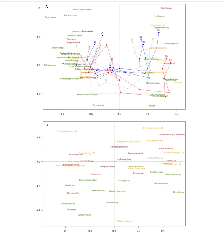
The 2-dimensional representation of the community (NMDS) showed a strong trend in time (plankton succession), and a divergence of this trend from ca. t25 between the high-pCO2
mesocosms and the low- and medium- ones (Figure 2).
Treatments followed a similar trend from t-3 until t17, but tended to separate afterwards, matching the simulated upwelling caused by deep water addition (t24). Permutation tests (with 999 permutations) did not show the areas (i.e., clusters of samples)
FIGURE 2 |Non-metric Multidimensional Scaling analysis (NMDS) of the plankton community (stress value = 0.18). Color code: blue = low-pCO2(M1, M5, and M9), gray = medium-pCO2(M3, M4, and M7), red = high-pCO2[M2, M6 (until t27), M8]. Only common species (>0.5% total abundances) represented. Taxa names:
phytoplankton (green), microzooplankton (yellow), mesozooplankton (burgundy). The numbers -3, 17, and 51 indicate sampling days; lines represent patterns.
Species are positioned in the graph according to their relative abundance during the experiment. Days of experiment included in the NMDS analysis were limited to t50, due to the absence of microZP samples for t56. Amplified area(B)is a zoom-in for a clearer view of the species that overlapped in the middle of the first graph [not shown in(A)for the sake of clarity].
representing the different pCO2 treatments to be significantly smaller than randomized areas, indicating that the variation due to CO2 is smaller than the changes over time (i.e., natural succession) (ANOSIM test,p-value = 0.246). Areas representing
the sampling day were significantly different from randomized areas using the same test, indicating a temporal trend (p-value = 0.001). Moreover, results for the interaction between sampling day and pCO2 treatment (ANOSIM test, p-value = 0.001)
matched with the NMDS, suggesting that there was a significant effect of pCO2 on plankton succession, ultimately affecting the plankton community development after the simulated upwelling event. Consequently, the plankton community developed differently within the different pCO2 treatments, the largest difference being in the high-pCO2mesocosms.
Zooplankton Temporal Trends
In view of zooplankton abundance and Chla levels we could define three experimental phases: pre-bloom (from t1 until deep water addition on t24), phytoplankton bloom phase (t25–35) and post-bloom phase (from t35 until the end of the experiment), as shown inFigure 1C.
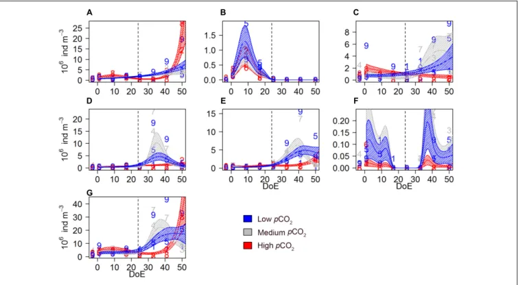
The microzooplankton (microZP) community comprised 13 different taxonomic groups of heterotrophic dinoflagellates and ciliates. Temporal trends of total microZP were affected bypCO2 [s(DoE):Treat, Table 2], resulting in higher abundances under the high-pCO2 treatment on the last sampling day. Averaged microZP abundances at the beginning of the experiment (t1) were 4.5·106 ± 2.89·106 individuals per m3 for the low-, 3.45·106 ± 8.03·105 for the medium-, and 4.07·106 ± 9.36·105for the high-pCO2treatments, respectively. After deep water addition (t24), abundances increased in all treatments, especially in the medium-pCO2 treatment. Maximum values were reached at the end of the experiment (t50) in the high- pCO2treatment with 2.14·107±8.94·106individuals per m3 (1.44·107±6.61·106and 1.52·107±1.08·107individuals per
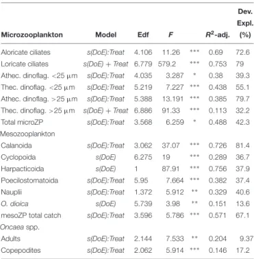
TABLE 2 |Zooplankton GAMM analyses.
Dev.
Expl.
Microzooplankton Model Edf F R2-adj. (%)
Aloricate ciliates s(DoE):Treat 4.106 11.26 ∗ ∗ ∗ 0.69 72.6 Loricate ciliates s(DoE)+Treat 6.779 579.2 ∗ ∗ ∗ 0.753 79 Athec. dinoflag.<25µm s(DoE):Treat 4.035 3.287 ∗ 0.38 39.3 Thec. dinoflag.<25µm s(DoE):Treat 5.219 7.227 ∗ ∗ ∗ 0.438 55.1 Athec. dinoflag.>25µm s(DoE):Treat 5.388 13.191 ∗ ∗ ∗ 0.385 79.7 Thec. dinoflag.>25µm s(DoE)+Treat 6.886 91.33 ∗ ∗ ∗ 0.113 32.2 Total microZP s(DoE):Treat 3.568 6.259 ∗ 0.488 42.3 Mesozooplankton
Calanoida s(DoE):Treat 3.062 37.07 ∗ ∗ ∗ 0.726 81.4
Cyclopoida s(DoE) 6.275 19 ∗ ∗ ∗ 0.289 36.7
Harpacticoida s(DoE) 1 87.91 ∗ ∗ ∗ 0.756 37.9
Poecilostomatoida s(DoE):Treat 5.95 7.664 ∗ ∗ ∗ 0.382 37.4
Nauplii s(DoE):Treat 1.372 5.912 ∗ ∗ 0.329 40.6
O. dioica s(DoE) 5.739 3.98 ∗ ∗ 0.151 13.6
mesoZP total catch s(DoE):Treat 3.596 5.786 ∗ ∗ ∗ 0.571 67.1 Oncaeaspp.
Adults s(DoE):Treat 2.144 7.533 ∗ ∗ 0.204 9.37 Copepodites s(DoE):Treat 2.062 5.914 ∗ ∗ ∗ 0.146 17.2 Models defined the temporal trend of the abundances alone [s(DoE)], or within an interaction with the pCO2treatments [s(DoE):Treat]. Only significant values (p- value<0.05) are presented. DoE, day of experiment; edf, estimated degrees of freedom; Dev. Expl., deviance explained. Significance codes:<0.001 ‘∗ ∗ ∗’ 0.001
‘∗ ∗’ 0.01 ‘∗’ 0.05.
m3 in the low- and medium- pCO2 treatments, respectively).
MicroZP responded rapidly to phytoplankton bloom formation following the simulated upwelling (t23/24) and showed the strongest increase in abundance in the medium-pCO2treatment.
On t50, however, abundances in the medium-pCO2 treatment decreased again while a pronounced increase in the high-pCO2
was observed (Figure 3G).
Aloricate ciliates, mainly represented by specimen<30µm, accounted for ∼26% on average of total microZP abundances.
Ciliate abundance was lower in high-pCO2 during the bloom phase and increased after t35, matching with Chla decrease (Figure 1). An effect ofpCO2on the temporal trend was detected on these ciliate abundances [s(DoE):Treat], indicating a direct link between CO2-enhanced phytoplankton growth and increases in ciliate abundance under high-pCO2 conditions (Table 2 andFigure 3A). Aloricate ciliates were clearly dominant while loricate ciliates, mainly represented by tintinnids, accounted for only ∼2.5% of total microZP abundance. No significant pCO2 effect was detected on the temporal trend of loricate ciliates [s(DoE)+Treat], even though abundances were higher at lower pCO2during the oligotrophic phase of the experiment (Table 2 andFigure 3B). Most dinoflagellates in low-and medium-pCO2 treatments responded to the deep-water addition and followed the Chlabuild-up and decrease (Figure 1) resulting in an increase in dinoflagellates abundance following the addition (t24), although only some (>25µm athecate) responded to high-pCO2
at the end of the experiment (Figures 3C–F). Small athecate dinoflagellate abundances (Figure 3C) were higher under high-pCO2 conditions during most of the oligotrophic phase, although highest abundances were recorded under medium- pCO2treatment toward the end of the experiment [s(DoE):Treat].
The most abundant group within the dinoflagellates were small thecate dinoflagellates. The best fitting model was an interaction ofpCO2and the temporal trend resulting in higher abundances at medium pCO2 in the second half of the experiment [s(DoE):Treat]. Thus, higher abundances of this group were recorded at medium- and low-pCO2 treatments during the bloom, followed by a subsequent decrease in the post-bloom phase (Table 2and Figure 3D). Large athecate dinoflagellates (Figure 3E) showed a similar trend during the bloom phase, but abundance resulted to be ultimately higher under low-pCO2 toward the end of the experiment [s(DoE):Treat]. Large thecate dinoflagellates (Figure 3F) responded differently than other dinoflagellates, reaching lowest abundance before deep water addition and increasing again when the phytoplankton bloom decayed, independent of thepCO2 treatment [s(DoE)+Treat].
Large dinoflagellates were mainly represented by the genus Gyrodinium, comprising∼12% of the total microZP abundances.
Small dinoflagellates from the genera Protoperidinium and Gymnodinium accounted for ∼22 and 20% total microZP abundances, respectively.
The mesozooplankton (mesoZP) community was dominated by copepods and comprised 28 different species or taxonomic groups (seeTable 3). Nauplii were counted from the net hauls (>55µm) and thus included in the mesoZP category, although we are aware that early copepod life stages would in principle belong to microZP when strictly followingSieburth et al.’s (1978)
FIGURE 3 |Microzooplankton abundances during the study period.(A)aloricate ciliates,(B)loricate ciliates,(C)small athecate dinoflagellates (<25µm),(D)small thecate dinoflagellates (<25µm),(E)large athecate dinoflagellates (>25µm),(F)large thecate dinoflagellates (>25µm),(G)total microZP. Color code:
blue = low-pCO2(M1, M5, and M9), gray = medium-pCO2(M3, M4, and M7), red = high-pCO2(M2, M6, and M8). DoE, day of experiment. Note that, for a better visibility of the data,y-axes have been adapted to abundances in each panel. Numbers represent abundances for the respective mesocosm (e.g., 9 for M9). Solid lines = prediction from Generalized Additive Mixed Models (GAMMs) (smoother trendsp-value<0.05); shaded area = confidence interval. Dashed line: t24, deep water addition.
size definition. Total mesoZP catch showed a different temporal trend for eachpCO2treatment [s(DoE):Treat,Table 2]. Averaged mesoZP abundances at the beginning of the experiment (t1) varied between 4730±1202 (low-pCO2), 6023±982 (medium- pCO2), and 5242 ± 369 (high-pCO2) individuals per m3, respectively. Our results showed that mesoZP abundances increased after deep water addition (t24), although this increase
TABLE 3 |Complete list of mesoZP species and taxa detected in the mesocosms registered throughout the study period.
(1) Foraminifera (15)Farranulaspp.
(2) Hydromedusae (16)Mecynocera clausi
(3)Muggiaeasp. (17)Microsetellaspp.
(4)Doliolumsp. (18)Nannocalanus minor
(5) Gastropoda larvae (19)Oithonaspp.
(6) Pteropoda (20)Oncaeaspp.
(7) Polychaete larvae (21)Rhincalanusspp.
(8) Polychaete (22)Temoraspp.
(9)Evadnesp. (23) Chaetognatha
(10) Copepoda nauplii (24) Cyprid larvae
(11)Acartiaspp. (25) Decapoda larvae
(12)Centropagesspp. (26) Echinodermata larvae
(13)Clausocalanusspp./Paracalanusspp. (27)Oikopleura dioica
(14)Corycaeussp. (28) Fish larvae
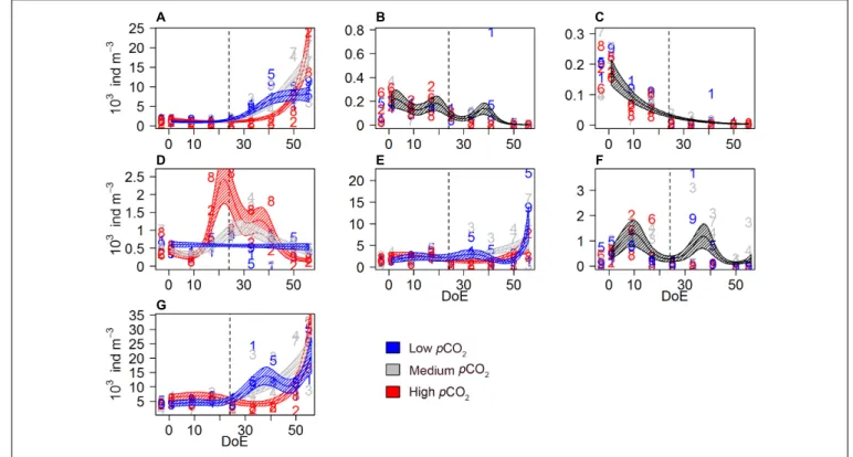
was delayed in the high-pCO2 treatment. Highest averaged abundances were recorded for all three treatments on the last sampling day (Figure 4): 23038 ±9230 individuals per m3 in low-pCO2, 25295±14196 in medium-pCO2and 24403±10928 in high-pCO2.
Different responses topCO2treatments were observed among the studied copepod orders. All copepods, including nauplii, represented ∼90% of total mesozooplankton abundances.
Calanoid copepods were mainly represented by Clausocalanus spp. andParacalanusspp. (including e.g.,Clausocalanus furcatus, C. arcuicornis, Paracalanus indicus), and accounted for 7–89%
(average = 38%) of the total mesozooplankton abundances. An increase in calanoid abundances was detected after deep water addition (t24) in low- and medium-pCO2. Calanoida evolved similarly within the low- and the medium-pCO2 treatments until ∼t40. Afterwards, abundances under medium-pCO2 and high-pCO2treatments increased, resulting in abundances higher than those in low-pCO2 mesocosms on the last sampling day (Figure 4A). Hence, a significant interaction betweenpCO2and temporal trend abundances was detected on calanoid abundances [s(DoE):Treat, Table 2] resulting in higher abundances under elevatedpCO2 conditions (medium- and high-) during the last two sampling days.
Cyclopoid copepods abundance (Figure 4B) decreased throughout the experiment independently of the treatment
FIGURE 4 |Mesozooplankton abundances during the study period.(A)Calanoida,(B)Cyclopoida,(C)Harpacticoida,(D)Poecilostomatoida,(E)copepod nauplii, (F)O. dioica,(G)mesoZP total catch. Color code: blue = low-pCO2(M1, M5, and M9), gray = medium-pCO2(M3, M4, and M7), red = high-pCO2(M2, M6, and M8). Note that the black lines indicate that the model prediction for the three treatments is the same. DoE, day of experiment. For a better visibility of the data, y-axes have been adapted to abundances in each panel. Numbers represent abundances for the respective mesocosm (e.g., 9 for M9). Solid lines = prediction from Generalized Additive Mixed Models (GAMMs) (smoother trendsp-value<0.05); shaded area = confidence interval. Dashed line: t24, deep water addition.
[s(DoE),Table 2]. This order of copepods was mainly represented byOithonaspp. Harpacticoid copepod abundances (Figure 4C) decreased from the start of the experiment, and nopCO2effect was detected [s(DoE), Table 2]. This order of copepods was only represented by Microsetella spp. during this experiment.
A significant effect ofpCO2on the temporal trend was detected on poecilostomatoid copepods (Figure 4D), mainly represented by Oncaea spp. [s(DoE):Treat, Table 2]. Poecilostomatoids abundance was highest in high-pCO2, increasing until∼t25 and decreasing gradually afterwards until the end of the experiment.
A similar trend was observed under medium-pCO2 while abundances under low-pCO2 conditions did not vary much during the experiment.pCO2had an effect on the temporal trend of nauplii abundances [s(DoE):Treat,Table 2], which accounted for∼33% of total mesozooplankton abundances. An increase in nauplii abundances under low- and medium-pCO2 conditions was detected after the deep-water addition (t24), with maximum abundances under the medium-pCO2treatment, while at high- pCO2 abundances did not increase until the last sampling day (Figure 4E).
The appendicularia population — represented by the species Oikopleura dioica— was mainly composed by juveniles and accounted for 0–40% (average = 8%) of total mesozooplankton catch. We could not detect a pCO2 effect on O. dioicaduring the experiment, even though they were completely absent in the high-pCO2treatment after deep water addition [s(DoE),Table 2
and Figure 4F]. The absence of a detectable effect could be attributed to the strong within-treatment variability.
Genus Oncaea
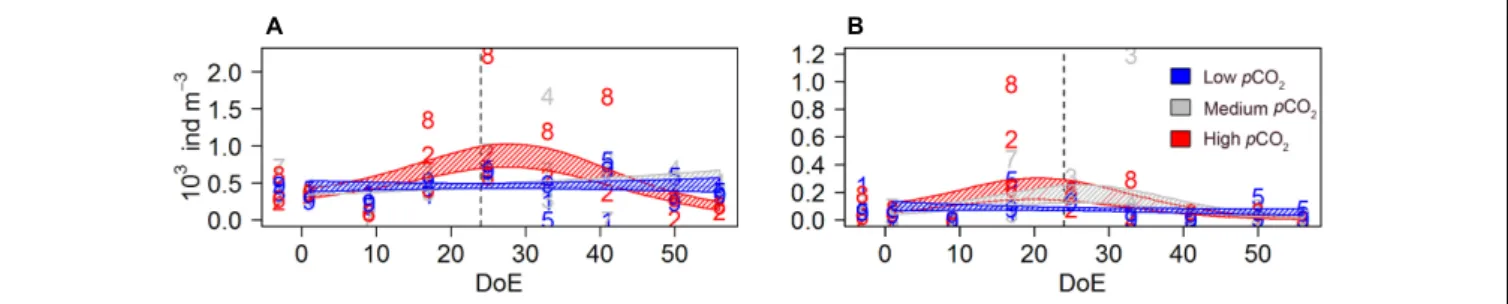
A significant effect ofpCO2on the temporal trend was detected on both adults and copepodites [s(DoE):Treat], although no reaction to deep water addition (t24) was observed. Elevated pCO2levels resulted in higher abundances for both adults (only under high-pCO2) and copepodites (under both medium- and high-pCO2conditions) (Figure 5andTable 2).
A GLMM detected a negative pCO2 effect on females’
sexual development, resulting in higher number of immature females under high- pCO2 conditions [s(DoE):Treat, Table 2 andFigure 6]. Approximately 60% of the females in the high- pCO2 mesocosms were classified as immature, versus ∼30%
in medium- and ∼36% low-pCO2 treatments over the whole duration of the experiment. The number of immature females at high- and low-pCO2 increased during the experiment while it decreased under medium-pCO2 (Figure 6A). There were no significant differences between the numbers of mature females without egg sacks across treatments (Figure 6B). In contrast, the number of females carrying eggs during the experiment was significantly different across treatments. At high-pCO2there were no egg-carrying females after t24, and a clear increase in numbers could only be detected at medium-pCO2 (Figure 6C).
Thus, we observed a clear negative effect at high-pCO2onOncaea
FIGURE 5 |Oncaeaspp. abundances during the study period.(A)Adults,(B)copepodites. Color code: blue = low-pCO2(M1, M5, and M9), gray = medium-pCO2
(M3, M4, and M7), red = high-pCO2(M2, M6, and M8). DoE, day of experiment. Numbers represent abundances per mesocosm (e.g., 9 for M9). Solid lines = prediction from Generalized Additive Mixed Models (GAMMs) (smoother trendsp-value<0.05); shaded area = confidence interval. Dashed line: t24, deep water addition.
FIGURE 6 |pCO2effect onOncaeaspp. females’ development and offspring (N).(A)number of immature females,(B)number of mature females (no egg sack),(C) number of egg-carrying females. Color code: blue = low-pCO2(M1, M5, and M9), gray = medium-pCO2(M3, M4, and M7), red = high-pCO2(M2, M6, and M8).
DoE, day of experiment. Solid lines = GLMM predictions (p-value>0.05). Dashed area = GLMM predictions confidence interval.
TABLE 4 |Oncaeafemales’ condition.
Oncaeafemales Model Edf Null deviance p-value Pseudo-R2
Number of immature females DoE:Treat 5 226.62 ∗ ∗ 0.620
Number of egg-carrying females DoE:Treat:egg sack 11 6.769 ∗ ∗ ∗ 0.598
Length of females (immature) DoE:Treat 5 17.97 ∗ ∗ 0.065
Length of females (mature) DoE:Treat:eggs 11 19.585 ∗ ∗ ∗ 0.104
Summary of GLMs on mature and immature individuals (n = 20 females per mesocosms). Models (GLMMs) defined the pCO2effect in time of Oncaea spp. females’
development and offspring DoE:Treat. DoE, day of experiment; edf, estimated degrees of freedom. Signif. codes: 0 ‘∗ ∗ ∗’ 0.001 ‘∗ ∗’ 0.01 ‘∗’ 0.05.
potential offspring (Table 4andFigure 6), represented by females carrying an egg-sack.
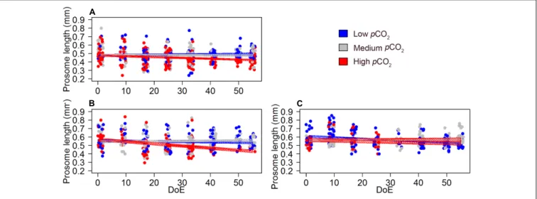
The model revealed a negative effect of thepCO2treatment on the prosome length of mature and immature Oncaea females (Table 4 and Figure 7), although this result must be taken with caution due to the relatively weak fit of our models (pseudo-R2 ∼0.1, Table 4). Pooling together mature and immature individuals, females’ prosome length was slightly shorter under high-pCO2 conditions (0.45±0.058 mm) when compared to medium-pCO2(0.56±0.085 mm) and low-pCO2 (0.52±0.082 mm).
Trophic Transfer Efficiency (TTE)
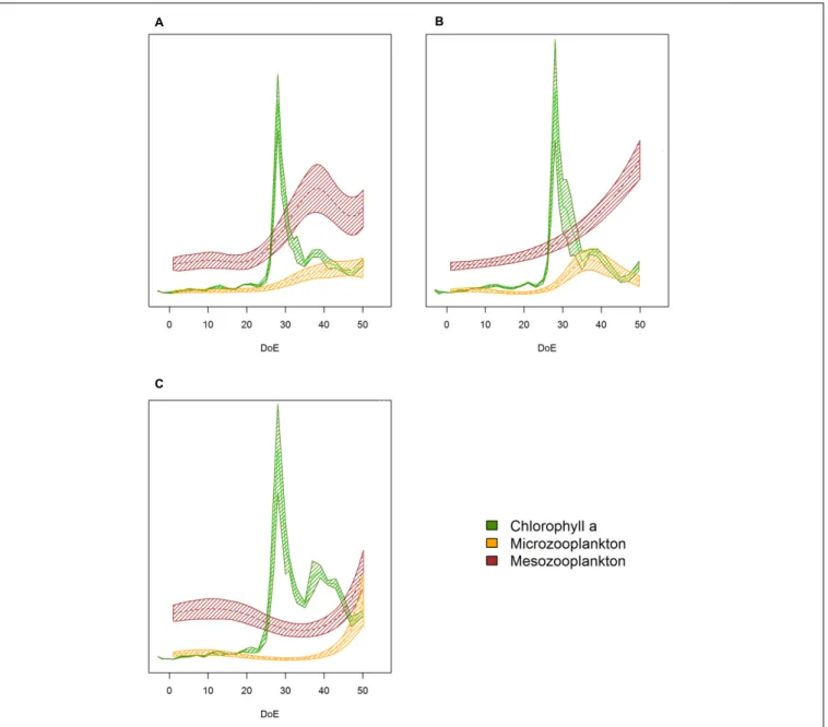
The simulated upwelling induced a phytoplankton bloom (t25–t35) and amplified differences in succession patterns and food-web structure under high-pCO2 conditions (Figure 8).
In the high-pCO2 mesocosms the phytoplankton bloom lasted for longer than in the other two treatments, and zooplankton responses were not detected until the bloom decayed (∼t48).
MicroZP abundance built up only in high-pCO2 treatment, while we observed an increase in mesoZP abundances in both medium- and high-pCO2 conditions toward the end of the experiment.
FIGURE 7 |pCO2effect onOncaeafemales’ development and offspring (length).(A)length of immature females,(B)length of mature females (no egg-sack),(C) length of egg-carrying females. Color code: blue = low-pCO2(M1, M5, and M9), gray = medium-pCO2(M3, M4, and M7), red = high-pCO2(M2, M6, and M8). DoE, day of experiment. Solid lines = GLMM predictions (p-value>0.05). Dashed area = GLMM predictions confidence interval.
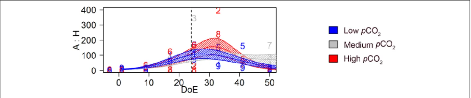
Generalized additive mixed models revealed a significant pCO2effect on the temporal trend of the A:H ratio [s(DoE):Treat, p-value < 0.05, Figure 9]. The model detected highest A:H ratio at the end of the phytoplankton bloom (∼t35) in the high-pCO2 treatment. During the post-bloom phase (i.e., after t35), the A:H ratio responded to the differential increase in microZP and mesoZP abundances (seeFigures 3G,4G). Hence, A:H in high-pCO2 decreased faster than in the other two treatments, overlapping low-pCO2 A:H on t50, when highest values corresponded to medium-pCO2treatment.
DISCUSSION
The main objective of this study was to analyze the effect of OA on the zooplankton community from subtropical waters during pre-bloom, bloom and post-bloom conditions. During the oligotrophic phase of this experiment we could not detect important differences in total zooplankton abundances between the treatments (Figures 3G, 4G). However, after the simulated upwelling, the zooplankton community under high- pCO2 conditions evolved significantly differently compared to the low- and medium-pCO2 conditions (Figure 2). Overall, higher zooplankton abundances were observed at elevatedpCO2 conditions (medium- and high-) in the post-bloom phase.
This result matches with a previous KOSMOS study in coastal mesotrophic conditions (Bach et al., 2016b) where certain groups of consumers capitalized on CO2-enhanced phytoplankton biomass, resulting in higher zooplankton abundances under moderate IPCC end-of-centurypCO2scenarios (RCP6.0) (Horn et al., 2016;Algueró-Muñiz et al., 2017). However, unexpectedly, both microZP and mesoZP abundances (Figures 3G, 4G) increased much later in the experiment under high-pCO2 than under medium- and low-pCO2. In the following, we will discuss the differences in zooplankton densities as well as the timing of bloom development.
pCO
2Effects on Zooplankton Densities
As reported by other authors (e.g.,Isari et al., 2015), responses to OA are not only dependent on species-specific sensitivities, but, much more importantly, depend on CO2 effects on the community and the trophic interactions taking place in a species’
natural habitat. In fact, most of the reported effects of OA on planktonic communities need to be attributed to these community effects, as many indicate a positive effect of OA (or rather carbon availability) on the plankton (Algueró-Muñiz et al., 2017;Taucher et al., 2017b). The temporal trends in major microZP groups (aloricate ciliates, small dinoflagellates) and Calanoida (Figures 3,4, respectively) were most likely triggered by the food supply for microZP combined with the preference of most copepods for heterotrophic protists (Suzuki et al., 1999;
Turner, 2004). As expected, picoplanktonic phytoplankton were a dominant component during the oligotrophic phase and large chain-forming diatoms dominated during the nutrient induced bloom (Taucher et al., 2017a). Diatoms are an ideal food source for larger mesoZP and this direct consumption of mesoZP on phytoplankton might have caused a release of microZP from grazing pressure after the deep-water addition.
The initial microZP abundance, as well as their taxonomic composition, was in agreement with those reported previously for the same area (Ojeda, 1998;Schmoker et al., 2014). During the post-bloom phase, microZP was dominated by dinoflagellates
<25 µm and aloricate ciliates. Ciliates and dinoflagellates are the main grazers on phytoplankton in marine systems, especially oligotrophic ones and also contribute to a large part to the copepod diets (Calbet, 2008). This is attributed to their appropriate size and high nutritional quality of microZP relative to phytoplankton (Stoecker and Capuzzo, 1990) and the dominance of small-sized phytoplankton in oligotrophic systems which is outside the food spectrum of many mesozooplankters (Kleppel, 1993). Previous OA studies reported a tolerance of microZP communities toward high CO2concentrations, or only
FIGURE 8 |Plankton succession trends.(A)Low-pCO2treatment,(B)medium-pCO2treatment,(C)high-pCO2treatment. Note that trends have been transformed to be in a 0 to 1 scale to enhance plankton succession visibility. Color code: green = Chla, yellow = microZP abundance, burgundy = mesoZP abundance. DoE, day of experiment. Solid lines = prediction from Generalized Additive Mixed Models (GAMMs) (smoother trendsp-value<0.05); shaded area = confidence interval.
very subtle changes in the community (Suffrian et al., 2008;
Aberle et al., 2013; Horn et al., 2016; Lischka et al., 2017) while other studies showed detrimental (Calbet et al., 2014) or even positive effects (Rose et al., 2009). In this study, an increase in aloricate ciliate abundances was observed in all treatments in response to the deep water-induced phytoplankton bloom, although the increase showed a considerable time-lag relative to the phytoplankton bloom, especially at high CO2
conditions. In contrast to aloricate ciliates, loricate ciliates played a minor role in this experiment and showed only a very small peak during the oligotrophic phase. Loricate ciliates started to decline after t10 and were virtually absent after deep water addition (seeFigure 3).
For dinoflagellates, especially small-sized athecates, we expected a positive effect of high-pCO2levels due to findings from previous OA studies conducted in oligotrophic (Sala et al., 2015) and eutrophic regions (Horn et al., 2016). During the oligotrophic phase of the experiment, this expectation was confirmed since higher abundances of small athecate dinoflagellates at high- pCO2were also found in our study. However, after deep water addition overall dinoflagellate abundances were higher at low- and medium-pCO2 conditions. Unlike ciliates, heterotrophic dinoflagellates are known to feed on phytoplankton of various sizes up to several times larger than their body size and have been shown to prey on bloom-forming diatoms including taxa as, e.g., Thalassiosira(Sherr and Sherr, 2007). The abundance
FIGURE 9 |Trophic transfer efficiency; autotrophy versus heterotrophy (A:H). Autotroph: heterotroph biomass ratio based on biomass estimations (µg C L−1). Color code: blue = low-pCO2(M1, M5, and M9), gray = medium-pCO2(M3, M4, and M7), red = high-pCO2(M2, M6, and M8). DoE, day of experiment. Solid
lines = prediction from Generalized Additive Mixed Models (GAMMs) (smoother trendsp-value<0.05); shaded area = confidence interval. Dashed line: t24, deep water addition.
of diatoms, however, was higher at high-pCO2compared to the low- and medium-pCO2conditions (Taucher et al., 2017a). Thus, the effect of high pCO2 on dinoflagellates was most likely an indirect one based on changes in the phytoplankton community and more precisely, on prey edibility (see section “pCO2Effects on Zooplankton Bloom Timing”).
Calanoida were positively affected by medium- and high- pCO2, although the trend was only visible during the last two sampling days. These results match with previous outcomes described for copepodites and adult Pseudocalanus acuspes in eutrophic waters andpCO2levels of∼760µatm (Algueró-Muñiz et al., 2017;Taucher et al., 2017b), suggesting a benefit of realistic end-of-centurypCO2levels on calanoid copepods through higher food availability. Small planktonic copepods are dominant in the plankton communities in many parts of the world’s oceans and therefore important members of pelagic food webs (Turner, 2004). Thus, a positivepCO2effect on these major zooplankton components could have a crucial impact on the transfer of energy to higher trophic levels thus affecting, e.g., future fisheries (Moyano et al., 2009;Sswat et al., 2018).
Copepod species that do not exhibit vertical migration behavior are considered as evolutionarily less exposed to high- pCO2 levels compared to other copepods, and typically more sensitive to OA (Fitzer et al., 2012; Lewis et al., 2013).
Accordingly, we expected cyclopoid (dominated by Oithona) and harpacticoid copepods (dominated byMicrosetella) to show lower abundances under elevated pCO2 conditions as neither species shows diel migration (Maar et al., 2006). However, during this experiment, elevatedpCO2did not cause a significant effect on Cyclopoida and Harpacticoida abundances, according to the GAMM analyses (Figures 4B,C). The reason for the decay in Cyclopoida and Harpacticoida abundances is not entirely clear but could be due to the distribution of the copepods in the water column, closer to the mesocosm sediment traps. Such a loss through sedimentation was previously observed in other mesocosm experiments during periods of low food availability (Bach et al., 2016a; Algueró-Muñiz et al., 2017). Oithona and Microsetellahave been reported to concentrate on marine snow (Ohtsuka et al., 1993;Koski et al., 2005) and during the present experiment, the cumulative flux of particulate organic matter to the sediment traps increased after deep water addition (Stange et al., 2018). This might have promoted a downward migration
of Microsetella—already from the beginning of the experiment on — to enhance their feeding on sinking material, preventing us to sample them in the net hauls.
pCO
2Effects on Zooplankton Bloom Timing
Where the observed response of the zooplankton densities is in line with previously published results, the differences in timing of the blooms were rather unexpected. In fact, zooplankton density increases after the simulated upwelling under high-pCO2 treatment were much slower than under the low and medium treatments. The most probable explanation for this observation lies in the differences in taxonomy of the phytoplankton responding to the nutrient addition of the upwelling. The phytoplankton bloom in the high-pCO2 mesocosms (M2 and M8) was dominated by Vicicitus globosus (Dictyochophyceae) which bloomed only in the high-pCO2 mesocosms from t25 until t47 (Riebesell et al., 2018). Harmful or non-edible for zooplankton, it seems likely that V. globosus caused adverse effects on the plankton community. MicroZP as potential grazers were most likely affected by the inadequacy of the available phytoplankton food (Chang, 2015), thus preventing the subsequent increase in mesoZP abundances. This is even more likely considering that once the phytoplankton bloom ceased in the high-pCO2 treatments, microZP started to increase in numbers at a time point when they were already decreasing at low and medium-pCO2. The tolerance to harmful algae has previously been described for copepod species closely related to those recorded in the mesocosms such as Paracalanus parvus (tolerant toChattonella antiqua) andOncaea venusta(tolerant to Karenia brevis) (Turner and Tester, 1989). AlthoughParacalanus sp. nauplii may exhibit adverse effects from feeding upon Alexandrium tamiyavanichii (Silva et al., 2013), we did not detect negative effects on nauplii abundances when relating them to the harmful algae abundance, but a delay in the reaction time likewise in aloricate ciliates, dinoflagellates and calanoid copepods. Accordingly, we based our conclusions for copepods on temporal trends andpCO2treatments rather than on possible effects of inedible/harmful food items. Our results suggest that copepods reacted to the different pCO2 levels only after their preferred prey [i.e., heterotrophic protists (Turner, 2004)] reacted