Travelling wave solutions for gravity fingering in porous media flows

Travelling wave solutions for gravity fingering in porous media flows

Koondanibha Mitra, Ben Schweizer, Andreas Rätz

Preprint 2020-05 Dezember 2020

Fakultät für Mathematik

Technische Universität Dortmund Vogelpothsweg 87

44227 Dortmund tu-dortmund.de/MathPreprints

gravity fingering in porous media flows

K. Mitra, A. R¨ atz, and B. Schweizer

November 10, 2020

Abstract: We study an imbibition problem for porous media.

When a wetted layer is above a dry medium, gravity leads to the propagation of the water downwards into the medium. In experiments, the occurence of fingers was observed, a phenomenon that can be described with models that include hysteresis. In the present paper we describe a single finger in a moving frame and set up a free boundary problem to describe the shape and the motion of one finger that propagates with a constant speed. We show the existence of solutions to the travelling wave problem and investigate the system numerically.

MSC: 76S05, 35C07, 47J40

Keywords: porous media, travelling waves, hysteresis

1 Introduction

Standard models for flow in unsaturated porous media fail in the description of a fundamental process, namely the imbibition into a dry medium with gravity as the driving force. While standard Richards models predict the formation of uniform imbibition fronts, the experimentally observed fingers [11, 26] can only be described with a model that incorporates hysteresis.

Models for incompressible unsaturated porous media flow typically use the water pressure p and the water saturation s as primary variables. The Darcy law for the velocity together with the mass balance equation leads to

∂

s = ∇ ⋅ ( k ( s )[∇ p + ge

]) , (1.1a) we refer to [2, 13, 22, 25] for the modelling. In the Richards equation (1.1a), the function k ∶ [ 0, 1 ] → R is the permeability function which has to be determined from experiments, g is the gravitational acceleration, e

is the normal vector pointing upwards. It is always assumed that s takes only values in [ 0, 1 ] .

Equation (1.1a) must be accompanied by a relation between saturation s and

pressure p. Models without hysteresis demand either the algebraic relation p = p

( s )

for some given function p

∶ [ 0, 1 ] → R ¯ , or they include the “τ -correction” and

demand, for some physical parameter τ > 0, known as the dynamic capillary number,

that p = p

( s )+ τ ∂

s; this latter model takes inertia in the material law into account,

see [12]. If, additionally, hysteresis in an imbibition process shall be modelled, a possible simple law is

∂

s = 1

τ [ p − p

( s )]

, (1.1b) where [⋅]

∶= max { 0, ⋅} denotes the positive part. Our aim is a travelling wave analysis of equation (1.1). We recall that p

∶ ( 0, 1 ) → R is a given imbibition capillary pressure function and τ > 0 is a given constant.

Regarding the modelling we note that, if both imbibition and drainage should be modelled, one replaces (1.1b) by the model of [4],

∂

s = 1

τ [ p − p

( s )]

+ 1

τ [ p − p

( s )]

. (1.2) Here, p

∶ ( 0, 1 ) → R is a drainage capillary pressure function with p

( s ) ≤ p

( s ) for all s ∈ ( 0, 1 ) , and [⋅]

∶= min { 0, ⋅} is the negative part function. Equation (1.2) is a hysteresis model since, pointwise in space and time, all pressure values in the closed interval [ p

( s ) , p

( s )] are permitted for a fixed saturation s. The play-type hysteresis model with dynamic capillary pressure was analyzed in [4, 15–17, 19, 21, 23, 24, 27].

Since we are interested in an infiltration problem with ∂

s ≥ 0, we restrict ourselves to the case p

( s ) = −∞ as in [9], i.e., we study (1.1b) instead of (1.2).

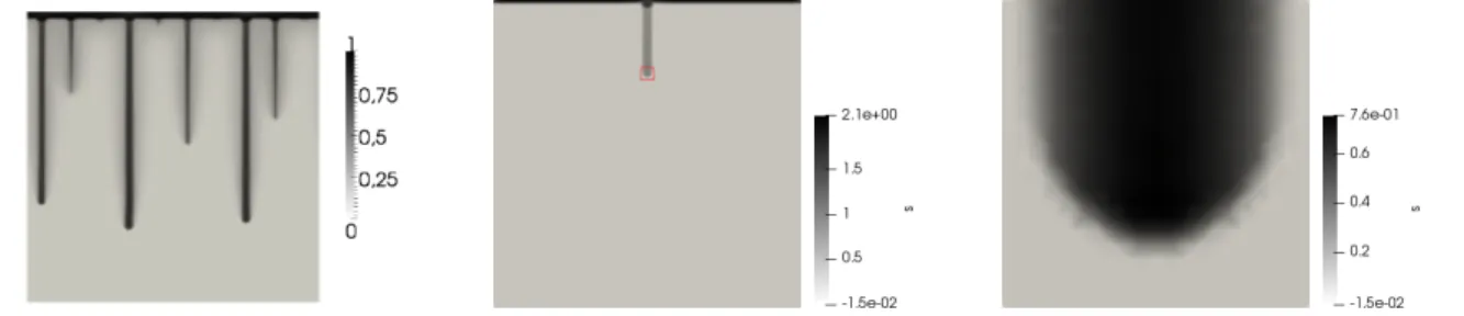
Figure 1: Motivation for this contribution. Left: A snapshot of a solution to the time dependent system (1.1). Fingers are clearly visible; the solution is comparible to experimental observations [21]. Middle: With another choice of boundary values and p

, a single finger is generated. A small squared region of size 2 × 2 around the finger-tip is marked [15]. Right: Enlargement of the marked region. We see the typical shape of the single finger in time-dependent calculations. The aim of this contribution is to analyze the travelling wave equations corresponding to (1.1) in order to obtain the shape of the single finger without a time-dependent calculation.

Numerical results for the time dependent system (1.1) are shown in Figure 1, originally published in [15, 21]. The figure illustrates a gravity driven imbibition process into an originally dry medium. Several fingers evolve in the process. It is observed that each finger travels approximately with constant speed. This has also been verified experimentally [26]. The present work aims at the description of a single finger in a co-moving frame of coordinates.

Travelling wave ansatz, domains and boundary conditions. Since we are

interested in imbibition fronts in columns of porous media, we choose a cylindrical

spatial domain Ω

. Restricting to two dimensions for convenience and denoting the

width of the cylinder by L > 0, we consider Ω

∶= ( 0, L ) × R ⊂ R

. Points in R

are

denoted as x = ( y, z ) . We seek time-dependent solutions to (1.1) that move with

a constant speed c > 0 in negative z-direction, i.e., downwards. This motivates the travelling wave coordinates

˜

z = z + ct , p ( y, z, t ) = p ( y, z ˜ ) , s ( y, z, t ) = s ( y, z ˜ ) . (1.3) In the following, we omit the tilde symbol and write z instead of ˜ z. The new coordinates transform system (1.1) into

c∂

s = ∇ ⋅ ( k ( s )[∇ p + ge

]) , (1.4a) cτ ∂

s = [ p − p

( s )]

. (1.4b) Even though the physical interpretation of a travelling wave solution requires the study of domains Ω

that extend to z → ±∞ , we choose here to study problem (1.4) on the semi-infinite domain

Ω ∶= ( 0, L ) × R

with bottom Σ ∶= ( 0, L ) × { 0 } = {( y, 0 ) ∶ 0 < y < L } . Truncations of the domain are necessary for numerical calculations and facilitate the analysis. The problem is translation invariant; one should consider the bottom Σ = { z = 0 } as being far below the finger.

The boundary data are given by a prescribed saturation s

> 0 and a prescribed pressure p

at the bottom Σ of the domain, and by a prescribed total influx F

on the top of the domain. More precisely, we assume that we are given s

∶ [ 0, L ] → [ 0, 1 ] , p

∶ [ 0, L ] → R , and F

∈ R

= ( 0, ∞) , and impose the boundary conditions

∫

L 0

k ( s ( y, z ))[ ∂

p ( y, z ) + g ] dy → F

as z → +∞ , (1.5a)

s = s

at z = 0 , (1.5b)

p = p

at z = 0 . (1.5c)

If the initial saturation of the medium is given by a number s

∈ ( 0, 1 ) , a natural choice for the boundary data is s

≡ s

and p

≡ p

( s

) . Along the lateral boundaries of Ω we impose homogeneous Neumann conditions (no flux).

Main results. We perform an analysis of the travelling wave problem (1.4)–(1.5) on Ω. For the most part of this article, we prescribe the relaxation parameter τ, the frame speed c, and the boundary data s

, p

, and F

. Only in our last result, Theorem 4.7, we choose c in dependence of the other parameters in order to satisfy a physically adequate flux condition on the lower boundary.

The first part of our results concerns the system (1.4)–(1.5) on the bounded truncated domain Ω

= ( 0, L )×( 0, H ) . We choose boundary conditions on the upper boundary appropriately and show that the system has a solution. The solution can be found with a variational principle, the analysis is given in Section 3.

The numerical part of this paper deals with this truncated problem. One result is the calculation of a finger solution, see Figure 2. The numerical method and the results are described in Section 5.

The limit H → ∞ for the solutions on the bounded domain is studied in Section

4. We find that every sequence of solutions ( s

, p

) to truncated domain problems

possesses a subsequence and a limit ( s, p ) which is a solution of the original problem

(1.4). The limit process shows an interesting dichotomy: In one case, the flux boundary condition for z → ∞ as in (1.5) remains satisfied (“large solution”). In the other case (“small solution”), only a corresponding inquality is satisfied.

The two cases are analyzed further. We find that “large solutions” are of the type that we would like to see in the fingering process: they possess a free boundary, the pressure p tends to −∞ as z → ∞ , and the solution is “large” in the sense that the saturation exceed a certain threshold. In the second case, the properties are reverted: The solution has a bounded pressure and it is “small” in the same sense as the solution was “large” in the other case. Interestingly, both types of solutions are found numerically, see Section 5.

Free boundary problem. Let us emphasize that we treat a free boundary problem. By (1.4b), one has to distinguish between the subdomain { x ∈ Ω ∣ ∂

s ( x ) >

0 } (expected to be in the bottom) and the subdomain { x ∈ Ω ∣ ∂

s ( x ) = 0 } (expected in the top part). In physical terms, this means that an imbibition process occurs near and below the finger-tip, whereas, in the region around the developed finger, the saturation does not change any more. With reference to the hysteresis relation, we note that the z-independent saturation implies that the pressure can take arbitrary values (below min p

( s ) ). Therefore, the pressure profile does not have to reflect the saturation profile and the fingers can remain stable in their upper part; no blurring by pressure differences occurs.

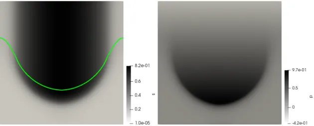
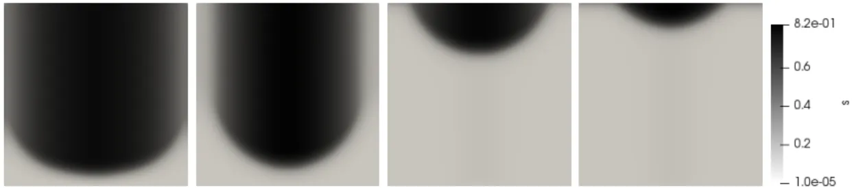
Figure 2: A numerical solution of the free boundary travelling wave problem. The gray scale indicates the values of the saturation s (left) and the pressure p (right).

The level line Γ = { x ∣ p = p

( s )} is marked in the left image. The line Γ shows the free boundary: Below the line, the saturation is increasing, above the line, the saturation remains constant (increasing in vertical direction and, hence, increasing in time when interpreted as a time dependent solution).

With Theorem 4.7 we provide the result that, for every F

within appropriate bounds, there exists a wave speed c such that a physical flux condition at the lower boundary is satisfied.

Literature. The classical porous media equation is obtained by setting τ = 0

and by replacing (1.1b) by the algebraic law p = p

( s ) . This classical equation is

interesting when the permeability coefficient is degenerate k ( 0 ) = 0. For existence

and uniqueness results in this classical case we refer to [1, 20]. The hysteresis model

(1.1b) was introduced in [3, 4, 12]. It combines dynamic effects (τ > 0) with a play- type hysteresis relation; the latter allows for an interval of pressure values p for a fixed saturation s. For a review of the modelling, we refer to [25].

For the model (1.1), well-posedness results have been obtained in one space dimension in [4], and in higher dimension in [15, 21]. Existence of solutions for an extension of the play-type model was shown in [16]. In [23], it was shown that the model does not define an L

-contraction; in this sense, it can explain the fingering effect. The fingers were found numerically for unsaturated media in [15], for the two-phase flow in [14]. Fingers were also observed numerically in [5, 7], where a free-energy based approach is used for modelling the capillary pressure. For a result with a degenerate p

-curve, see [24]. A uniqueness result was derived in [6].

Travelling waves for the model have been analyzed in [17, 19, 27]. An analysis for pure imbibition (∂

s ≥ 0 allows to set p

( s ) = −∞ ) was previously performed for one space dimension in [9]. The present work extends the results to two space dimensions. Let us note that the methods are independent of the dimension and that, up to notation, the results remain valid, e.g., in three space dimensions. The dimension enters only in Sobolev embeddings that are used for regularity statements in the appendix.

2 Preliminaries

The coefficient functions k and p

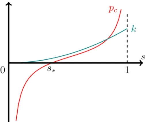
are fixed throughout this work. We make as- sumptions that are quite common and consistent with experiments, see [13]. For an illustration see Figure 3.

Assumption 2.1. The functions k ∶ [ 0, 1 ] → [ 0, ∞) and p

∶ ( 0, 1 ) → R satisfy:

(Ass-pc) The function p

is differentiable and for some ρ > 0 holds p

≥ ρ on ( 0, 1 ) . Upon normalization of the pressure, we can set p

( s

) = 0 for a given saturation value s

∈ R . We assume p

( s ) → −∞ as s ↘ 0 and p

( s ) → ∞ as s ↗ 1.

(Ass-k) The function k is differentiable, k ∣

∈ C

, and k

( . ) , k

( . ) > 0 on ( 0, 1 ) .

p

k

s

1

0

s

Figure 3: Typical functions p

and k.

The free boundary description. What qualitative behavior can we expect for solutions of the travelling wave problem (1.4)–(1.5)? We expect that the pressure stabilizes, as z → +∞ , to an affine function with ∇ p ≈ − g

e

. If s (and hence k ( s ) ) does not depend on z, then both sides of (1.4a) can vanish. This is what we expect for solutions in the upper part of the domain. We will be interested in solutions ( p, s ) that satisfy, for some h ∈ R

,

∂

s = 0 and p ≤ p

( s ) for all ( y, z ) with y ∈ ( 0, L ) and z > h . (2.1) For such a solution we can define a function Ψ ∶ [ 0, L ] → [ 0, ∞) as

Ψ ( y ) ∶= inf { z

> 0 ∣ ∂

s ( y, z ) = 0 for all z ≥ z

} . (2.2) The graph of Ψ is a part of the free-boundary, {( y, Ψ ( y ))∣ y ∈ ( 0, L )} ⊂ Γ. For the rest of the paper, we define the function s

∶ [ 0, L ] → [ 0, 1 ] as

s

( y ) ∶= lim

z→∞

s ( y, z ) . (2.3)

By positivity ∂

s ( y, z ) ≥ 0 and boundedness of s, the function s

is well-defined for solutions ( s, p ) of (1.4). When a solution satisfies (2.1), there holds s ( y, z ) = s

( y ) for all z > h.

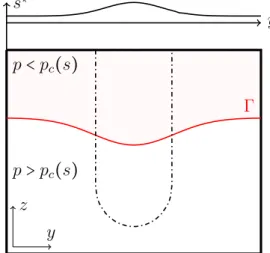
Γ p < p

( s )

p > p

( s ) z

y

y s

Figure 4: When interpreted as a solution of the time-dependent problem, the finger moves with a constant speed downwards. The dashed line represents the boundary of the finger; one may think of an isoline of the saturation. The graph at the top part of the Figure indicates a profile of the limiting saturation s

as defined in (2.3).

We refer to Figure 4 for an illustration. It is important not to confuse the free boundary Γ with the shape of the finger (the region of high saturation). We emphasize that the saturation profile remains unchanged (independent of z) above Γ; in particular, the finger extends to z → +∞ .

Relations in the travelling wave formulation. A fundamental problem in

travelling wave analysis is the determination of free parameters, in our case the

wave speed c. The other parameters are fixed: τ, g > 0 are physical constants, L > 0

a geometrical constant, and the boundary conditions fix F

> 0 and s

> 0. In the

travelling wave formulation, c ≥ 0 is a further unknown of the system. Nevertheless, for the most part of our analysis, we fix boundary values s

and p

and treat the problem with prescribed c. Only in our final result we determine c from an additional boundary condition for z → −∞ .

Let us collect some properties of the real parameters.

Lemma 2.2 (Wave speed and limiting pressure in the doubly infinite domain). Let ( s, p ) ∈ C

( Ω

) × C

( Ω

) be a classical solution to (1.4) on Ω

with the boundary condition (1.5a) and the two conditions s → s

and k ( s )∇ p → 0 as z → −∞ . Then, with s

as in (2.3), the wave speed satisfies

c = ( F

− k ( s

) gL ) /(∫

( s

( y ) − s

) dy ) . (2.4) If the solution possesses a free boundary, i.e. (2.1) holds for some h > 0, then

g

∶= g − ( F

/∫

k ( s

( y )) dy ) (2.5) satisfies g

> 0 and there holds ∇ p ( y, z ) + g

e

→ 0 as z → ∞ for every y ∈ ( 0, L ) . Proof. Integrating (1.4a) over ( 0, L ) × (− H, H ) yields

c ∫

L 0

s ( y, z ) dy ∣

H

z=−H

= ∫

k ( s ( y, z ))[ ∂

p ( y, z ) + g ] dy ∣

H z=−H

.

Sending H → ∞ provides (2.4).

Relation (2.1) implies that s ( y, z ) = s

( y ) holds for z > h. Therefore, the elliptic equation reduces to

∇ ⋅ ( k ( s

)∇ p ) = 0 in ( 0, L ) × ( h, ∞) . (2.6) In particular, the flux quantity ∫

k ( s

) ∂

p ( y, z ) dy is independent of z for z > h.

The boundary condition (1.5a) allows to evaluate this flux for z → ∞ ; we find

∫

L 0

k ( s

( y )) ∂

p ( y, z ) dy = F

− g ∫

L 0

k ( s

( y )) dy = − g

∫

L 0

k ( s

( y )) dy . (2.7) This provides that, for z > h, the weighted average of ∂

p coincides with − g

.

Solutions p of the elliptic equation (2.6) with homogeneous Neumann boundary conditions on unbounded domains have the property that ∇ p stabilizes to a constant as z → ∞ (a consequence of the strong maximum principle for ∂

p). Relation (2.7) shows that this constant is − g

e

.

Let us assume for a contradiction g

< 0. Then p is a growing function for z → ∞ . This is in contradiction with (1.4b), in which the left hand side vanishes for z > h and p

( s ) is independent of z for z > h.

Let us now assume g

= 0 in order to exclude also this case. We use a maximum

principle for p in the interior of the set {( y, z )∣ ∂

s = 0 } = {( y, z )∣ p ≤ p

( s )} . The

minimum of p is attained at the boundary. At the lower boundary of this set,

there holds p = p

( s ) . This implies that the minimum is attained in a point of

the form ( y, z ) = ( y, Ψ ( y )) . We now use, for any ε > 0, the strong maximum

principle: p ( y, Ψ ( y ) + ε ) > p ( y, Ψ ( y )) = p

( s ( y, Ψ ( y ))) = p

( s ( y, Ψ ( y ) + ε )) . This

implies p > p

( s ) in ( y, Ψ ( y ) + ε ) and hence ∂

s ( y, Ψ ( y ) + ε ) > 0, in contradiction to

the construction of Ψ.

Notation. Together with the domain Ω = ( 0, L ) × R

with bottom boundary Σ = ( 0, L )×{ 0 } we also use, for any H > 0, the bounded domain Ω

∶= ( 0, L )×( 0, H ) with the top boundary Σ

∶= ( 0, L )×{ H } . We recall that we always impose homogeneous Neumann conditions at the lateral boundaries { 0 } × R

and { L } × R

(accordingly for the truncated domain).

The function sign ∶ R → { 0, 1 } is defined as sign ( u ) ∶= 0 for u ≤ 0, and sign ( u ) ∶= 1 otherwise. The letter C denotes a generic positive constant and the value may change from one line to the next in calculations. We already introduced [ q ]

= max { 0, q } = ( q + ∣ q ∣)/ 2 and [ q ]

= min { 0, q } = −[− q ]

.

3 Existence result for bounded domains

Let τ > 0, s

∈ ( 0, 1 ) , and two functions p

∈ H

( Σ ) ∩ C

( Σ ¯ ) and s

∈ H

( Σ ) be given. We assume s

≤ s

≤ 1 and p

≥ p

( s

) . For a height parameter H > 0 we introduce the following truncated problem.

Definition 3.1 (Truncated domain travelling wave problem). Let c, F

> 0 be given.

A pair ( s, p ) ∈ H

( Ω

) × H

( Ω

) on the domain Ω

= ( 0, L ) × ( 0, H ) with upper boundary Σ

and lower boundary Σ is a truncated domain travelling wave solution (T W

-solution) if there holds

c∂

s = ∇ ⋅ ( k ( s )[∇ p + ge

]) in Ω

, (3.1a) cτ ∂

s = [ p − p

( s )]

in Ω

, (3.1b)

s = s

, p = p

on Σ , (3.1c)

p ≡ p

∈ R on Σ

, (3.1d)

∫

k ( s )[ ∂

p + g ] = F

. (3.1e)

We emphasize that the constant pressure value p

∈ R is a free parameter and part of the solution of the problem.

We note that for every T W

-solution ( s, p ) , the flux quantity

F

( z ) ∶= ∫

k ( s ( y, z ))[ ∂

p ( y, z ) + g ] − cs ( y, z ) dy (3.2) is independent of z ∈ ( 0, H ) by (3.1a). Evaluating this flux in the upper and in the lower boundary provides, by (3.1e),

∫

k ( s

) ∂

p + ∫

( k ( s

) g − cs

) = F

− ∫

cs . (3.3)

Remark 3.2. Let us give a sloppy description of the consequences of (3.3) for small

boundary data s

. There is the possibility that ∂

p is large at Σ. This means that

a sharp transition occurs near the lower boundary. In the opposite case (without

boundary layer), the left hand side of (3.3) is small. In this case, a moderate flux

F

> 0 forces the system that s is not small at Σ

. This is the desired behavior for

finger-like travelling wave solutions; they should connect a small saturation at z = 0

with a moderate or large saturation at z = H.

Remark 3.3 (A condition for the wave speed c). Let us highlight another conse- quence of the fact that F

of (3.2) is independent of z. When ( s, p ) is a solution on the doubly unbounded domain Ω

then we expect, in the limit z → −∞ , that s → s

, p → p

( s

) , and ∂

p → 0. In this situation, the constant flux quantity is necessarily F

= ( gk ( s

) − cs

) L.

We use this observation in order to choose a closure condition for the case when the speed c is treated as an unknown: Even when we solve a Dirichlet problem in the truncated domain Ω with boundary conditions s

and p

at the lower boundary Σ, we will seek for c and solutions to the Dirichlet problem that satisfy the additional relation

F

= ∫

( k ( s

)[ ∂

p + g ] − cs

) = ( gk ( s

) − cs

) L . (3.4) Theorem 4.7 yields that, given s

, p

, s

, and F

, we find a speed c such that (3.4) is satisfied.

In the remainder of this section, we seek for T W

-solutions ( s, p ) . We use the space of functions

H

( Ω

) ∶= { u ∈ W

( Ω

)∣ tr ( u ) = 0 on Σ , ∃ u

∈ R ∶ u = u

on Σ

} . (3.5) The weak formulation of (3.1a) and (3.1e) is:

∫

c∂

s φ + ∫

k ( s )[∇ p + ge

] ⋅ ∇ φ = ∫

F

φ for all φ ∈ H

( Ω

) . (3.6) Theorem 3.4 (Existence of T W

-solutions to prescribed data). Let H, c, τ, F

> 0 and s

∈ ( 0, 1 ) be given, let p

∈ H

( Σ ) ∩ C

( Σ ¯ ) and s

∈ H

( Σ ) satisfy

s

≤ s

< 1 , and 0 < p

− p

( s

) on Σ .

Then there exists a T W

-solution ( s, p ) with s, ∂

s ∈ L

( Ω

) , p ∈ H

( Ω

)∩ H

( Ω

) . Proof. We use an iteration over saturation fields.

Definition of the iteration. Let there be given a saturation field s

∈ Y ∶= { s ∈ L

( Ω

) ∣ s

≤ s ≤ 1 } .

We define the coefficient functions a ∶= k ( s

) and b ∶= p

( s

) on Ω

. We seek a solution p of

1

τ [ p − b ]

= ∇ ⋅ ( a [∇ p + ge

]) in Ω

, (3.7) with the boundary conditions p = p

on Σ and (3.1d)–(3.1e). This solution can be found with a variational method. We define the space of admissible functions as X

∶= { u ∈ H

( Ω

) ∣ u = p

on Σ , ∃ u

∈ R ∶ u = u

on Σ

} and minimize the func- tional

A ∶ X

→ R , A ( p ) ∶= ∫

1

2τ [ p − b ]

+ 1

2 a ∣∇ p + ge

∣

− F

∫

p . (3.8) The functional is convex and coercive, which implies that a minimizer p exists. The Euler-Lagrange equation for p reads

∫

1

τ [ p − b ]

ϕ + a [∇ p + ge

] ⋅ ∇ ϕ = F

∫

ϕ ∀ ϕ ∈ H

( Ω

) .

Since arbitrary compactly supported test-functions ϕ can be inserted, equation (3.7) holds for p. The Euler-Lagrange equation additionally encodes the boundary con- dition ∫

a ( ∂

p + g ) = F

. Given p

= p, we can solve the family of ordinary differential equations

cτ ∂

s = [ p

− p

( s )]

, (3.9) with initial data s = s

on z = 0; this system is related to (3.1b) together with the first equation in (3.1c). We denote the solution of this system by s =∶ s

.

Fixed point of the iteration. We claim that, for some constant C = C ( H, c, τ ) independent of s

, the pressure p = p

satisfies

∥ p ∥

+ ∥∇ p ∥

≤ C . (3.10) In order to show this estimate, we first choose an H

-extension ˆ p

of the data p

, vanishing at the upper boundary. We can now multiply equation (3.7) with p − p ˆ

and integrate to obtain

∫

1

τ [ p − b ]

([ p − b ] − p ˆ

+ b ) + ∫

( a [∇ p + ge

]) ⋅ ∇( p − p ˆ

) = ∫

F

p . One of the integrals on the left hand side is an upper bound for k ( s

)∥∇ p ∥

, the other term with quadratic growth in p is on the left hand side and positive because of [ p − b ]

[ p − b ] ≥ 0. The remaining terms have linear growth in p and can therefore be estimated with Youngs inequality and with the Poincar´ e inequality.

The corresponding solutions s

= s of the ordinary differential equation satisfy 0 ≤ s ≤ 1 by the growth assumption on p

. In particular, there holds s

∈ Y . With R ∶= ∣ Ω

∣

= ∣ LH ∣

, we find that the above construction provides a map

T ∶ Y ⊃ B

( 0 ) → B

( 0 ) ⊂ Y , s

↦ s

.

We claim that the map T is compact. We will show the compactness below with the characterization of compact subsets of L

( Ω

) by Kolmogorov-Riesz. An application of Schauder’s fixed point theorem yields the existence of the desired solution s.

Let us turn to compactness of T . We consider the family p = p

of solutions for s = s

∈ B

( 0 ) . This family of solutions is bounded in H

( Ω

) , hence the finite differences p ( y, . ) − p ( y + δ, . ) ∈ L

(( 0, H ) ; R) are small for δ > 0 small, independent of s. More precisely,

∫

L−δ

0

∫

H

0

∣ p ( y, z ) − p ( y + δ, z )∣

dz dy ≤ η ( δ ) ,

with η ( δ ) → 0 as δ → 0, independent of s. We now consider two solutions of the ordinary differential equation (3.9), s ( y, . ) and s ( y + h, . ) to inputs p ( y, . ) and p ( y + h, . ) . The solutions differ only as much as their right hand sides and their initial values differ. Because of our assumption s

∈ H

( Σ ) , we therefore find also for the solutions

∫

∫

∣ s ( y, z ) − s ( y + δ, z )∣

dz dy ≤ Cη ( δ ) .

On the other hand, since ∂

s is bounded in L

( Ω

) , the corresponding estimate

∫

∫

∣ s ( y, z + δ ) − s ( y, z )∣

dz dy ≤ Cη ( δ ) is clear. This shows compactness of the

image set of s-fields.

4 Unbounded domain solutions for H → ∞

In this section we analyze the solutions ( s

, p

) in the limit H → 0. Again, for the larger part of this section, we keep τ > 0, s

∈ ( 0, 1 ) , F

, and c > 0 fixed;

only in Theorem 4.7 we determine c from the other parameters. The main result of this section is the following: Let ( s

, p

) denote the T W

-solution as discussed in Theorem 3.4. Then, for H → ∞ , there holds ( s

, p

) → ( s, p ) in an appropriate sense for some limit pair ( s, p ) , which is defined on the unbounded domain Ω. The pair ( s, p ) is a travelling wave solution for the semi-infinite domain Ω.

It turns out that two different limiting solution types are possible. Type I is the “large solution”. It is characterized by the following properties: 1) The solution is large in the sense that ∫

gk ( s ( y, z

)) dy ≥ F

for some z

. This means that a certain F

-dependent threshold is exceeded by the saturation variable. 2) The solution has a free boundary: For some h > 0 there holds ∂

s ( y, z ) = 0 for every z ≥ h. 3) The solution has an unbounded pressure, p → −∞ as z → ∞ .

Accordingly, Type II solutions are the “small solutions”. They have a bounded pressure and no free boundary.

To proceed with the analysis, we consider different assumptions.

Assumption 4.1. The following properties can be considered for the solution se- quence ( s

, p

) of (3.1), obtained in Theorem 3.4.

Bounds for parameters The limiting saturation s

∈ ( 0, 1 ) , the wave speed c, and the flux F

satisfy

gk

( s

) < c < g ( k ( 1 ) − k ( s

))/( 1 − s

) , (4.1a) gL [ k ( s

) + k

( s

)( 1 − s

)] < F

< gLk ( 1 ) . (4.1b) Bound for the pressure For a real number p ¯ < ∞ independent of H holds

p

≤ p ¯ in Ω

. (4.2)

Local bound for the gradient There exists C

> 0 such that, for every H > 0,

∥∇ p

∥

≤ C

. (4.3) Regularity The saturation has the regularity properties

s

, ∂

s

∈ H

( Ω

) . (4.4) The assumptions have a quite different character. Inequalities (4.1) are ranges for the physical parameters; we expect the existence of travelling waves in this parameter regime. The uniform upper bound of (4.2) is expected to hold, but it should be derived from the system of equations, which we did not succeed to do.

The regularity estimate (4.3) and the local regularity (4.4) can be shown with the tools of elliptic regularity theory, see [10]. We formulate them here as assumptions, since the regularity theory is not the focus of this contribution.

We note that the relations (4.2)–(4.3) imply three further estimates:

∥ s

∥

≤ s ¯ ∶= p

( p ¯ ) < 1 . (4.5a)

In Lemma A.3 we prove that, for a constant C

= C

( C

, s

, p

) ,

∥∇ s

∥

≤ C

. (4.5b) Since (4.5b) provides ∥ ∂

s

∥

< C

, one also has from (3.1b) that

p

≤ p

( s

) + cτ C

in Ω

. (4.5c) Our main result on unbounded domains is the following.

Theorem 4.2 (Limits of T W

-solutions). Let c, F

, τ > 0, s

∈ ( 0, 1 ) , and boundary data s

, p

∈ C

( Σ ) with s

≤ s

< 1 and p

( s

) < p

be given. Let all the properties of Assumption 4.1 be satisfied. For a sequence H → ∞ , let ( s

, p

) be solutions to (3.1). Then, for a limiting pair ( s, p ) , there holds ( s

, p

) → ( s, p ) locally in L

( Ω ) . The limits satisfy s ∈ C

( Ω ) , ∂

s ∈ L

( Ω ) , p ∈ H

( Ω ) ∩ H

( Ω ∪ Σ ) , ( s, p ) = ( s

, p

) on Σ, and (1.4). The solution ( s, p ) is either of Type I or of Type II:

Type I: “Large solution” The solution has a free-boundary: There exists h ∈ R

such that ∂

s = 0 for all y ∈ ( 0, L ) and z ≥ h. The solution is large in the sense that, with s

( y ) ∶= lim

s ( y, z ) , there holds g ∫

k ( s

( y )) dy ≥ F

, with strict inequality if p, s, and ∂

s are continuous. Furthermore, p ( y, z ) → −∞

as z → ∞ in this case.

Type II: “Small solution” The solution has a bounded pressure, there holds p ∈ L

( Ω ) . Furthermore, ∇ p ∈ L

( Ω ) . The solution is “small” in the sense that g ∫

k ( s

( y )) dy ≤ F

.

Type I solutions satisfy additionally the boundary condition (1.5a).

The theorem follows from Propositions 4.4 and 4.5. Before we can prove these results, we have to establish an a priori estimate, which is the basis for both propo- sitions.

Lemma 4.3 (A priori estimate for T W

-solutions). Let F

, c, τ, s

> 0 and s

, p

∈ C

( Σ ) with s

≤ s

( y ) < 1 and p

( s

) < p

. For a sequence 0 < H → ∞ , let ( s

, p

) be solutions to (3.1). We assume that the solution sequence satisfies relations (4.3) and (4.4). We use the characteristic functions 1

∶= 1

and 1

∶= 1

on Ω

. There exists a constant C

∶= C

( c, τ, s

, p

, C

) , independent of H, such that

∫

1

p

( s

)∣∇ s

∣

+ ∫

1

pc′(p⁻¹_c (pH))

∣∇ p

∣

+ cτ ∫

∣∇ s

∣

≤ C

. (4.6a) If, additionally, (4.2) is satisfied, there exists C

∶= C

( c, τ, s

, p

, C

, p ¯ ) such that

∫

1

∣∇ p

∣

+ ∫

∣∇( ∂

s

)∣

≤ C

. (4.6b)

Proof. Within this proof, we write ( s, p ) instead of ( s

, p

) to have shorter formulas.

With C > 0 we refer to generic constants that may depend on c, τ, s

, p

, C

, p, but ¯

not on H.

Step 1: Test function K ( s ) . We use K ∶ [ 0, 1 ] → [ 0, ∞) , defined as K ( s ) ∶=

∫

k ( % )

d%. Equivalently, we may say that K is the primitive of k

, satisfying K

( s ) = 1

k ( s ) , K ( 0 ) = 0 .

Below, we will use additionally the primitive of K ; we denote by ˜ K the function that satisfies ˜ K

( s ) = K ( s ) and ˜ K ( 0 ) = 0.

We use K ( s )( y, z ) = K ( s ( y, z )) as a test function in (3.1a) and study c ∫

K ( s ) ∂

s = ∫

K ( s )∇ ⋅ ( k ( s )[∇ p + ge

]) .

Using an integration by parts, we may write this relation as c ∫

∂

K ˜ ( s ) + ∫

k ( s )[∇ p + ge

] ⋅ ∇ K ( s )

= ∫

K ( s ) k ( s )[ ∂

p + g ] − ∫

K ( s

) k ( s

)[ ∂

p + g ] . (4.7) We have constructed K such that ∇ K ( s ) = k ( s )

∇ s. This gives a simple formula for the second integral. With another integration by parts and with 1 = 1

+ 1

we find

c ∫

K ˜ ( s ) − c ∫

K ˜ ( s

) + ∫

1

∇ p ⋅ ∇ s + ∫

1

∂

p ∂

s + ∫

ge

⋅ ∇ s

= ∫

K ( s ) k ( s ) ∂

p − ∫

K ( s

) k ( s

) ∂

p + g ∫

K ( s ) k ( s ) − g ∫

K ( s

) k ( s

) . (4.8) We note that the last two integrals on the right hand side and the first two integrals on the left hand side are bounded. Since we assumed (4.3), actually the entire right hand side of (4.8) is bounded. The last integral of the left hand side can be integrated, which shows that also this term is bounded. We therefore find

∫

1

∇ p ⋅ ∇ s + ∫

1

∂

p ∂

s ≤ C . (4.9) We want to rewrite the first integral. With this aim, we observe that cτ ∂

s = [ p − p

( s )]

in Ω

implies cτ ∇ ∂

s = (∇ p − p

( s )∇ s )1

(we recall that we assumed

∂

s ∈ H

( Ω ) ). This yields

∫

1

∇ p ⋅ ∇ s = cτ ∫

∇ s ⋅ ∇ ∂

s + ∫

1

p

( s )∣∇ s ∣

. (4.10) The first term on the right hand side of (4.10) is

cτ ∫

∇ s ⋅ ∇ ∂

s = cτ ∫

∂

( 1

2 ∣∇ s ∣

) = cτ

2 ∫

∣∇ s ∣

− cτ

2 ∫

∣∇ s ∣

= cτ

2 ∫

∣∇ s ∣

− 1

2cτ ∫

[ p

− p

( s

)]

− cτ

2 ∫

∣ ∂

s

∣

. (4.11) At this point, we obtained from (4.9)

∫

1

∂

s ∂

p + ∫

1

p

( s )∣∇ s ∣

+ cτ

2 ∫

∣∇ s ∣

≤ C . (4.12)

Step 2: Test function Φ. We next consider the new test function Φ ∶= [ K ( s ) − K ( p

( p ))]

∈ H

( Ω

) .

Note that ∂

s > 0 ⇐⇒ p > p

( s ) ⇐⇒ p

( p ) > s ⇐⇒ K ( p

( p )) > K ( s ) . This shows

Φ = [ K ( s ) − K ( p

( p ))]1

.

Using Φ as a test function for (3.1a) and exploiting that Φ ≠ 0 only when ∂

s = 0, we find

∫

Φ ∇ ⋅ ( k ( s )[∇ p + ge

]) = c ∫

Φ∂

s = 0 . (4.13) Also on the left hand side, the term Φ ∇⋅[ k ( s ) ge

] = Φk

( s ) g∂

s vanishes identically.

Integration by parts in (4.13) yields, using Φ = 0 on Σ,

∫

k ( s )∇ Φ ⋅ ∇ p = ∫

Φk ( s ) ∂

p . (4.14) Because of ∇ Φ = (

∇ s −

∇ p ) 1

, we find

∫

∇ s ⋅ ∇ p 1

− ∫

k ( s ) k ( p

( p ))

∣∇ p ∣

p

( p

( p )) 1

= ∫

Φ k ( s ) ∂

p . (4.15) The first integral is ∫

∇ s ⋅ ∇ p 1

= ∫

∂

s ∂

p 1

, hence it coincides with the first term in (4.12). Since k ( s )1

> k ( p

( p ))1

, from (4.12) we arrive at

∫

1

p^′_c(pc−1(p))

∣∇ p ∣

1

+ ∫

1

p

( s )∣∇ s ∣

+ cτ

2 ∫

∣∇ s ∣

≤ C , (4.16) where we exploited once more (4.3). At this point, we have shown (4.6a).

Step 3: Test function ∂

s. To show (4.6b), we use the test function ∂

s =

1

cτ

[ p − p

( s )]

∈ H

( Ω

) in (3.1a). With an integration by parts we obtain 1

cτ ∫

k ( s )∇ p ⋅ ∇[ p − p

( s )]

= ∫

∂

s k ( s ) ∂

p − ∫

∂

s k ( s

) ∂

p + ∫

( gk

( s ) − c )∣ ∂

s ∣

.

(4.17)

We observe that, by (4.3) and (4.5b), the first two integrals on the right hand side are bounded. Furthermore, the middle term of (4.16) shows that also the last integral is bounded.

Using the algebraic manipulation 2a ( a − b ) = a

− b

+ ( a − b )

, the left hand side of (4.17) is written as

1

cτ ∫

k ( s )∇ p ⋅ ∇[ p − p

( s )]

= 1

cτ ∫

k ( s )∇ p ⋅ (∇ p − ∇ p

( s ))1

= 1

2cτ ∫

k ( s )[∣∇ p ∣

+ ∣∇( p − p

( s ))∣

− ∣∇ p

( s )∣

]1

= 1

2cτ ∫

k ( s )[1

∣∇ p ∣

+ ( cτ )

∣∇( ∂

s )∣

− 1

( p

( s ))

∣∇ s ∣

] .

Inequality (4.16) along with (4.5a) shows that the negative term has a bounded

integral. This shows (4.6b) and concludes the proof.

To investigate the free-boundary structured solution described in Theorem 4.2 we define the function h ∶ R

→ R

with (2.1) in mind: For H > 0 and ( s

, p

) solving (3.1), h = h ( H ) is defined as

h ( H ) ∶= inf { z

∈ [ 0, H ] ∶ ∂

s

= 0 a.e. in ( 0, L ) × ( z

, H )} . (4.18) The height h marks a horizontal line such that, above that line, ∂

s vanishes. We note that h ∈ [ 0, H ] is well-defined and that h = H is possible.

Proposition 4.4 (Free-boundary solutions). We consider the situation of Theo- rem 4.2 with a sequence ( s

, p

) of T W

-solutions for H → ∞ . Additionally, we assume for the sequence H → ∞ that the height

h ( H ) is bounded. (4.19)

Under this assumption, a free-boundary travelling wave solution ( s, p ) exists. More precisely, there exists a pair ( s, p ) with s ∈ C

( Ω ) , ∂

s ∈ L

( Ω ) , p ∈ H

( Ω )∩ H

( Ω ∪ Σ ) , satisfying (1.4)–(1.5). The solution is of free boundary type in the sense that there exists h

> 0 such that ∂

s = 0 for all y ∈ ( 0, L ) and z ≥ h

. The flux satisfies

F

≤ g ∫

L 0

k ( s

( y )) dy . (4.20)

Under the additional regularity assumptions s, ∂

s, p ∈ C

( Ω ) , the strict inequality holds in (4.20).

Proof. Let h

> 0 denote an upper bound of the function h ( H ) , i.e.

h ( H ) ≤ h

for all H. (4.21)

Step 1: An additional a priori estimate. We consider once more the function s

( y ) = s

( y, h

) for all y ∈ ( 0, L ) . (4.22) Let g

∈ R be the number

g

∶= g − ( F

/∫

k ( s

( y )) dy ) , (4.23) and let ˜ p

∈ H

( Ω

) be the function

˜

p

( y, z ) ∶= p

( y, z ) + g

z for ( y, z ) ∈ Ω

. (4.24) We note that these definitions reflect the observations of Lemma 2.2. We finally define ϕ

∈ C

([ 0, 1 ]) as the function

ϕ

( s ) ∶= cs − ( g − g

) k ( s ) . (4.25) This allows to write (3.1a) in the form

∇ ⋅ [ k ( s

)∇ p ˜

] = ∂

ϕ

( s

) . (4.26)

We observe that, by (3.1e) and the choice of g

in (4.23),

∫

k ( s

) ∂

p ˜

= F

+ ( g

− g ) ∫

k ( s

) = 0 . (4.27) The test function ˜ p

in (4.26) provides the identity

∫

p ˜

∇ ⋅ [ k ( s

)∇ p ˜

] = ∫

p ˜

∂

ϕ

( s

) . (4.28) The left hand side of (4.28) is calculated with an integration by parts, exploiting the fact that p

on the upper boundary is constant, p

≡ p

on Σ

. In the last line of the calculation we use (4.27).

∫

p ˜

∇ ⋅ [ k ( s

)∇ p ˜

]

= − ∫

k ( s

)∣∇ p ˜

∣

+ ∫

p ˜

k ( s

) ∂

p ˜

− ∫

p ˜

k ( s

) ∂

p ˜

= − ∫

k ( s

)∣∇ p ˜

∣

+ ( p

+ g

H ) ∫

k ( s

) ∂

p ˜

− ∫

p

k ( s

)[ ∂

p

+ g

]

= − ∫

k ( s

)∣∇ p ˜

∣

− ∫

p

k ( s

)[ ∂

p

+ g

] .

The right hand side of (4.28) is treated with two integrations by parts,

∫

p ˜

∂

ϕ

( s

)

= − ∫

ϕ

( s

) ∂

p ˜

+ ∫

p ˜

ϕ

( s

) − ∫

p ˜

ϕ

( s

)

= − ∫

ϕ

( s

) ∂

p ˜

+ [∫

∂

p ˜

ϕ

( s

) + ∫

p

ϕ

( s

)] − ∫

p

ϕ

( s

)

= ∫

( ϕ

( s

) − ϕ

( s

)) ∂

p ˜

+ ∫

( ϕ

( s

) − ϕ

( s

)) p

.

Boundedness of many of the above terms can be concluded from the facts that g

is bounded, ϕ

∈ C

([ 0, 1 ]) , and boundedness of ∂

p from (4.3). From (4.28) and Young’s inequality we obtain

∫

k ( s

)∣∇ p ˜

∣

≤ C − ∫

( ϕ

( s

) − ϕ

( s

)) ∂

p ˜

≤ C + ∫

1

2k ( s

) ∣ ϕ

( s

) − ϕ

( s

)∣

+ ∫

k ( s

)

2 ∣ ∂

p ˜

∣

.

We have applied Young’s inequality in such a way that the last term on the right hand side can be substracted from both sides. Since ϕ

( s

) − ϕ

( s

) = 0 holds for z ≥ h

, the first integral on the right hand side is bounded. We conclude

∫

k ( s

)∣∇ p ˜

∣

≤ C ( 1 + h

) .

Recalling additionally the estimates from Lemma 4.3, we have the following esti- mates for the solution sequence:

∫

[∣∇ p ˜

∣

+ ∣ ∂

s

∣

+ ∣∇ ∂

s

∣

] ≤ C . (4.29)

Step 2: Limit equations. It remains to exploit the bounds of (4.29) to construct the limit solution for H → ∞ . Since the sequence g

is bounded, we can choose a subsequence { H

}

with lim H

= ∞ and g

∈ R such that g

→ g

. In the following, we only use this subsequence. The estimate (4.29) allows to choose a further subsequence and a pair ( s, p ) with s ∈ H

( Ω )∩ L

( Ω ) and p ∈ H

( Ω ) such that, for any bounded compact subset Ω

⊂ Ω, there holds

s

→ s and ∂

s

→ ∂

s strongly in L

( Ω

) , (4.30a) p

⇀ p weakly in H

( Ω

) and p

→ p strongly in L

( Ω

) . (4.30b) These convergences imply that also the limit ( s, p ) satisfies (1.4) in Ω and the boundary conditions at the lower boundary. Furthermore, ∂

s

≡ 0 for all H on { z ≥ h

} implies ∂

s ≡ 0 on { z ≥ h

} .

Step 3: Flux relations. Regarding the flux we use that the quantity

F

( z ) ∶= ∫

k ( s

( y, z ))[ ∂

p

( y, z ) + g ] − cs

( y, z ) dy (4.31) is independent of z ≥ 0 (compare F

in (3.2)). Since the saturation s

is independent of z for z ≥ h

, also the quantity

F

( z ) ∶= ∫

k ( s

( y, z ))[ ∂

p

( y, z ) + g ] dy (4.32) is independent of z for z ≥ h

. Because of this independence and because of F

( H ) = F

, we find, as H → ∞ , for every z ≥ h

,

F

= F

( z ) → ∫

k ( s ( y, z ))[ ∂

p ( y, z ) + g ] dy . (4.33) This shows that the boundary condition (1.5a) is satisfied by the limit functions.

We have found a free boundary solution on an unbounded domain. As in Lemma 2.2, there follows g

≥ 0 and, under the regularity assumptions s, ∂

s, p ∈ C

( Ω ) , the strict inequality g

> 0. This implies F

= ( g − g

) ∫

k ( s

( y )) dy ≤ g ∫

k ( s

( y )) dy, and hence (4.20).

Proposition 4.5 (Bounded pressure solutions). Let the situation be that of Theo- rem 4.2, with T W

-solutions ( s

, p

) along a sequence H → ∞ . We assume here that the sequence of heights h ( H ) diverges,

h ( H ) → ∞ as H → ∞ . (4.34)

Then, a bounded pressure travelling wave solution ( s, p ) exists. More precisely, there exists a pair ( s, p ) with s ∈ C

( Ω ) , ∂

s ∈ L

( Ω ) , p ∈ H

( Ω ) ∩ H

( Ω ∪ Σ ) satisfying (1.4). For C > 0 there holds

∥ p ∥

+ ∥∇ p ∥

+ ∥ ∂

s ∥

≤ C . The solution satisfies

g ∫

k ( s

( y )) dy ≤ F

. (4.35)

We note that we do not obtain the flux condition (1.5).

Proof. In this proof, we only write H → ∞ and h → ∞ for the two sequences. We furthermore use Ω

= [ 0, L ] × ( 0, h ) .

Step 1: L

-bound for the pressure. The upper bound for the pressure was assumed in (4.2), p

≤ p ¯ in Ω

. Our aim in this step is to show a lower bound for the pressure.

On the lower boundary Σ there holds p

= p

≥ 0. We claim that there is a lower bound also along the upper boundary Σ

of Ω

. Indeed, by definition of h in (4.18), there is a subset of non-vanishing measure in ( 0, L ) × ( h − 1, h ) on which ∂

s

> 0 holds, i.e. p

> p

( s

) ≥ 0. The Lipschitz bound (4.3) implies that p

≥ − C

holds on Σ

for C

= C

√

1 + L

.

We can now exploit a maximum principle to obtain

− C

≤ p

≤ p ¯ a.e. in Ω

. (4.36) The maximum principle is derived by using [ p

+ C

]

as a test function in (3.1a), which results in

∫

[ p

+ C

]

∇ ⋅ [ k ( s

)∇ p

] = ∫

[ p

+ C

]

( c − gk

( s

)) ∂

s

. An integration by parts yields

∫

k ( s

)∣∇[ p

+ C

]

∣

= ∫

[ p

+ C

]

k ( s

) ∂

p

− ∫

[ p

+ C

]

k ( s

) ∂

p

+ ∫

[ p

+ C

]

( c − gk

( s

)) ∂

s

.

As analyzed before, the boundary terms vanish because of p

+ C

≥ 0 along Σ and along Σ

. Regarding the last integral we note that in every point x with ∂

s ( x ) > 0, there holds p

( x ) ≥ p

( s

( x )) ≥ p

( s

) = 0, and hence [ p

+ C

]

= 0. This shows that all terms on the right hand side vanish. We obtain (4.36).

Step 2: A further a priori estimate. From the uniform pressure bound (4.36) we conclude that p

( p

) is bounded away from 1. With this information, the bound of (4.6a) provides, with a constant C > 0 independent of H, the inequality

∫

1

∣∇ p

∣

+ ∫

1

p

( s

)∣∇ s

∣

≤ C . Similarly, (4.6b) implies

∫

1

∣∇ p

∣

+ ∫

∣∇( ∂

s

)∣

≤ C.

Combining both of these inequalities with (4.36), and recalling ∂

s

= 0 in Ω

∖ Ω

, we obtain

max

Ω^h

∣ p

∣

+ ∫

∣∇ p

∣

+ ∫

[∣ ∂

s

∣

+ ∣∇ ∂

s

∣

] ≤ C . (4.37)

Step 3: Limit H → ∞ . Because of h → ∞ , we find a limiting pair ( s, p ) such

that the local convergences of (4.30) hold for any compact subset Ω

of Ω. It is

straightforward to verify that ( s, p ) solves (1.4). Moreover, (4.37) together with

h → ∞ implies the additional properties ∇ p ∈ L

( Ω ) (as a bounded solution to an

elliptic equation) and ∂

s ∈ L

( Ω ) .