Traveling wave solutions for the Richards equation with hysteresis

Traveling wave solutions for the Richards equation with hysteresis

E. El Behi-Gornostaeva, K. Mitra, B. Schweizer

Preprint 2018-05 September 2018

Fakultät für Mathematik

Technische Universität Dortmund Vogelpothsweg 87

44227 Dortmund tu-dortmund.de/MathPreprints

equation with hysteresis

E. El Behi-Gornostaeva ¹ , K. Mitra ² , B. Schweizer ¹

September 24, 2018

Abstract: We investigate the one-dimensional non-equilibrium Richards equation with play-type hysteresis. It is known that regu- larized versions of this equation permit traveling wave solutions that show oscillations and, in particular, the physically relevant effect of a saturation overshoot. We investigate here the non-regularized hysteresis operator and combine it with a positive τ -term. Our result is that the model has monotone traveling wave solutions.

These traveling waves describe the behavior of fronts in a bounded domain. In a two-dimensional interpretation, the result character- izes the speed of fingers in non-homogeneous solutions.

MSC: 76S05, 74N30, 35C07

Keywords: porous media, hysteresis, traveling wave, saturation overshoot

1 Introduction

When water is infiltrating a porous medium, the process can show a homogeneous saturation front or the formation of fingers; in the latter case, water enters preferen- tially along thin channels of high water saturation. We study a mathematical model for unsaturated flow in porous media. We investigate a non-equilibrium Richards equation with hysteresis, a model that allows the formation of fingers.

We are interested in the propagation of saturation profiles and restrict ourselves to the one-dimensional case. The main result of this contribution is that there exist, for appropriate parameter ranges, monotone traveling wave solutions for the system.

In the case of a homogeneous front, the traveling wave describes the propagation of the front. In the case of fingering, the traveling wave describes the saturation profile in one finger. Our results predict the speed of the finger, but they also yield that, possibly after a transition time, no overshoot occurs in the finger tip, even in the case of a positive redistribution time τ.

1

Fakult¨ at f¨ ur Mathematik, TU Dortmund, Vogelspothsweg 87, 44227 Dortmund, Germany

2

Department of Mathematics and Computer Science, TU Eindhoven, PO Box 513 5600 MB

Eindhoven, The Netherlands

Before we compare our results with the existing literature, we formulate the model problem. Spatial points of the one-dimensional system are denoted by x ∈ R , time instances are denoted by t ∈ [0, ∞). The physical state in (x, t) is described by two variables: saturation ˜ s and pressure ˜ p. The tilde marks functions that depend on space and time, ˜ s, p ˜ : R × [0, ∞) → R in the case of entire domains. Combining Darcy’s law with mass conservation yields the unsaturated media flow equation

∂

˜ s = ∂

[k(˜ s)(∂

p ˜ + 1)] . (1.1) In this equation, we have normalized the porosity of the medium. Gravity points in negative x-direction and is also normalized. The hydraulic conductivity k is a given coefficient function s 7→ k(s); it is a nonnegative and nondecreasing function.

Equation (1.1) is complemented with a constitutional law that relates pressure and saturation. Models for slow processes without hysteresis use an algebraic rela- tion: With a given capillary pressure function p

one demands ˜ p = p

(˜ s). We can include non-equilibrium effects (τ > 0) and play-type hysteresis (γ > 0) in the form

˜

p ∈ p

(˜ s) + γ(˜ s) H(∂

˜ s) + τ ∂

˜ s . (1.2) In this relation, [0, 1] 3 s 7→ p

(s) ∈ R is a given non-decreasing function, the capillary pressure curve for imbibition. The real parameter τ ≥ 0 is a measure for a redistribution time in the microscopic geometry. The function γ : [0, 1] → [0, ∞) is a measure for the hysteretic width; one often uses a constant function and writes γ ∈ [0, ∞). The multivalued function H is the step function

H(ζ) :=



 

 

0 for ζ > 0 , [−1, 0] for ζ = 0 ,

−1 for ζ < 0 .

In the equilibrium case τ = 0, the model imposes that imbibition (∂

˜ s > 0) occurs always with the imbibition capillary pressure ˜ p = p

(˜ s), while drainage (∂

s < ˜ 0) occurs always with the drainage capillary pressure ˜ p = p

(˜ s) − γ(˜ s).

The above model (1.1)–(1.2) has received considerable attention in recent years.

It was suggested and studied in [1, 7] as a natural extension of the Richards equation.

It is thermodynamically consistent and includes the hysteresis effect with a play- type model. We note that Richards emphasizes in his famous article of 1931 the importance of hysteresis. For an overview regarding hysteresis modelling and the development of the mathematical theory see [17].

Further research on (1.1)–(1.2) was mainly performed along three different lines:

A. Analysis of the hysteresis system in arbitrary dimension and fingering effect.

It was shown that the above system is well-posed for constant γ and positive per- meability k [11], that solutions are unique [2], that the system does not define an L

-contraction (and hence allows for the fingering effect) [16], and that it indeed can produce the fingering effect, see e.g. [14]. Two-phase flow equations are treated in [3] and [10]. For a stability analysis for the system without hysteresis see e.g. [6].

B. Numerical methods. The numerical investigations of [8] and [18] are per-

formed in order to detect the occurance of saturation overshoots (see below in part

s p

0 1

p

(s)

p

(s) − γ(s)

Figure 1: Sketch of the constitutive relation between saturation s and pressure p using play-type hysteresis (τ = 0).

C) and their dependence on the data of the problem. Saturation plateaus are re- covered in [18]. In [15], a numerical scheme is suggested for a version of the above equations with non-vertical scanning curves. Indeed, introducing third order splines as scanning curves seems to facilitate the Newton iterations in a numerical scheme.

A numerical analysis of a discontinuous Galerkin scheme is performed in [9].

C. One-dimensional analysis and saturation overshoots. Much of the analysis in this field (including this contribution) is motivated by the effect of saturation overshoots: Experiments show that an imbibition front can be non-monotone. In this case, the saturation directly behind the front is higher than at larger distance (behind the front) [5]. Even though the experimental results come with large errors, one may interpret that the saturation forms plateaus. This is consistent with the shape of solutions to Riemann problems and is well understood in the case of two- phase flow equations [22]. It is also well understood that a positive parameter τ in (1.2) can produce non-monotone profiles, see [4, 19] for systems without static hysteresis, and [21, 12] for the full system. The methods are based on phase-space analysis of ordinary differential equations. For an early result in a problem with adsorption, see [20].

Traveling waves

In order to discuss traveling waves in further detail, we specify initial and boundary conditions for the above systems. Let 0 < s

∈ R denote the initial saturation and 0 < F

∈ R prescribe an inflow at the top boundary (x = +∞). We then complement (1.1)–(1.2) by

˜

s(x, 0) = s

for every x ∈ R , (1.3a)

˜

s(x, t) → s

as x → −∞ for every t ∈ (0, ∞) , (1.3b)

k(˜ s(x, t))[∂

p(x, t) + 1] ˜ → F

as x → +∞ for every t ∈ (0, ∞) . (1.3c)

Much of the one-dimensional analysis is concerned with traveling wave solutions.

In the traveling wave ansatz, one seeks profile functions s, p : R → R and a scalar velocity c > 0 such that the time-dependent functions have the special form

˜

s(x, t) := s(x + ct) , p(x, t) := ˜ p(x + ct) . (1.4) Equations (1.1)–(1.2) provide the following system for s, p : R → R and c > 0:

c∂

s = ∂

[k(s)(∂

p + 1)] , (1.5) p ∈ p

(s) + γH(∂

s) + τ c∂

s , (1.6) where we used H(c∂

s) = H(∂

s) for positive c ∈ R . The boundary conditions are

s(ξ) → s

as ξ → −∞ , (1.7a)

k(s(ξ))[∂

p(ξ) + 1] → F

as ξ → +∞ . (1.7b) Main result. Our main result regards traveling waves in the case that drainage does not occur. This happens in the physical experiment when γ is large compared to the front width. Mathematically, we set γ = +∞ in the system or, formally more correct: We replace (1.6) by the two conditions:

p(ξ) = p

(s(ξ)) + τ c∂

s(ξ) if ∂

s(ξ) > 0 , (1.8a) p(ξ) ≤ p

(s(ξ)) + τ c∂

s(ξ) if ∂

s(ξ) = 0 , (1.8b) and we demand ∂

s(ξ) ≥ 0 for all ξ ∈ R . We emphasize that the case γ = +∞ is of physical relevance in the effect of gravity fingering, see the discussion in Section 4.

Essentially, our main result states that for every s

∈ (0, 1) and every small flux F

> 0, there exists a monotone traveling wave solution s, p : R → R and c > 0.

Theorem 1.1. Let k and p

be coefficient functions as specified in Assumption 2.2 below. Let s

∈ (0, 1) and F

> 0 be boundary data of the problem. With c

= k

(s

) as in (3.6) we demand that the flux satisfies the bounds k(s

)+c

(1−s

) < F

< k(1).

We use c ¯ = ¯ c(k, s

, F

) from relation (3.17) below.

There exists a critical value τ

= τ

(k, p

, s

, F

) ≥ 0 such that, for every τ > τ

, there exists a velocity c ∈ (c

, ¯ c) and a traveling wave solution (s, p) to the system (1.5), (1.7), and (1.8).

2 Reformulation of the traveling wave equations

We will construct solutions to (1.5), (1.7), and (1.8) in a special form: We obtain

saturation profiles s that are constant for ξ > 0 and pressure profiles p that are affine

for ξ > 0. The following lemma provides a simplified set of equations. Solutions to

the simplified equations can be extended as indicated above to find solutions to the

original problem.

Lemma 2.1 (Traveling wave equations on a half space). Let F

, s

> 0 be boundary data and let s

> 0 satisfy k(s

) ≥ F

. For c > 0 let (s, p) : (−∞, 0] → R × R be a classical solution of the ordinary differential equation

c(s − s

) = k(s) [∂

p + 1] − k(s

) (2.1a)

p = p

(s) + τ c∂

s (2.1b)

on (−∞, 0), satisfying the conditions

s(ξ) → s

as ξ → −∞ , (2.2a)

s(0) = s

, (2.2b)

∂

s(0) = 0 , (2.2c)

c(s

− s

) + k(s

) = F

. (2.2d)

We furthermore assume that the function ξ 7→ s(ξ) is monotonically increasing on (−∞, 0).

If we extend s and p for ξ > 0 by setting

s(ξ) = s

, (2.3a)

p(ξ) = F

k(s

) − 1

ξ + p

(s

) , (2.3b)

then the extended functions (s, p) : R → R × R solve the system (1.5), (1.7)–(1.8).

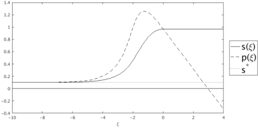
A numerically computed solution as in Lemma 2.1 is depicted in Figure 2.

Figure 2: A numerically computed traveling wave solution. The figure shows the saturation profile as a solid line and the pressure profile as a dashed line. The solution is computed for p

(s) = s, k(s) = s

, τ = 5, s

= 0.1, F

= 0.25. We obtain numerically c = 0.2139 and s

= 0.8013.

Proof. (a) Equations on (−∞, 0). Differentiating (2.1a) yields

c∂

s = ∂

[k(s)(∂

p + 1)]

on (−∞, 0), which is (1.5). We demanded that s is monotonically increasing on (−∞, 0), hence ∂

s > 0 holds and we are always in the first case of (1.8) on that interval. Therefore (2.1b) implies (1.8) on (−∞, 0).

(b) Boundary conditions. Condition (2.2a) is equivalent to (1.7a). In order to verify (1.7b), we differentiate (2.3b). We obtain for any ξ > 0

k(s(ξ))(∂

p(ξ) + 1) = F

,

since s(ξ) ≡ s

by (2.3a). This yields (1.7b).

(c) Equations on (0, ∞). The extensions of s and p in (2.3) are defined in such a way that ∂

s ≡ 0 and ∂

p + 1 ≡ F

/k(s

) holds on (0, ∞). Since k(s) is constant, we see that both sides of equation (1.5) vanish.

We check that (1.8) holds on (0, ∞): There holds ∂

s ≡ 0, hence we are in the second case of (1.8). The pressure satisfies p ≤ p

(s

) by definition in (2.3b) and the assumption F

/k(s

) ≤ 1. By s ≡ s

we have verified (1.8).

(d) Equations in 0. We evaluate equation (2.1a) in ξ = 0 and insert (2.2b) to obtain

c(s

− s

) = k(s

)(∂

p(0) + 1) − k(s

) . Condition (2.2d) provides the value of the flux in 0,

k(s

)(∂

p(0) + 1) = F

. (2.4)

Both, the saturation s and the flux quantity [k(s)(∂

p + 1)] are continuous in ξ = 0.

This implies that (1.5) holds in all of R .

In the following section we obtain our main result. We will show that, given F

, s

> 0, we find c > 0, s

> 0 with k(s

) ≥ F

, and s solving (2.1)–(2.2). We derive this result under the following assumptions on the functions k and p

. Assumption 2.2. Let the coefficient function k : [0, 1] → [0, ∞) be of class C

, non-decreasing and strictly convex, positive on (0, 1]. Let the coefficient function p

: (0, 1) → R be of class C

with p

(s) > 0 for all s ∈ (0, 1). We furthermore assume p

(s) → ∞ for s % 1.

We remark that also other p

-functions can be treated with our methods. We find the same results when the last part of Assumption 2.2 is replaced by: p

(s) → ζ ∈ R for s % 1 and p

is multi-valued with p

(1) = [ζ, ∞).

3 Existence of hysteretic traveling wave solutions

In view of Lemma 2.1, our aim in the following is to construct solutions to system (2.1)–(2.2). The equations (2.1) can be written as

∂

s p

!

= (p − p

(s))/(cτ ) (c(s − s

) + k(s

))/k(s) − 1

!

. (3.1)

With the function

G(s) := G(s; c, s

) := c(s − s

) + k(s

)

k(s) − 1 , (3.2)

we can write the unknowns and the right hand side as y :=

s p

: (−∞, 0] → R

, G(y) :=

(p − p

(s))/(cτ ) G(s)

, (3.3)

and the dynamical system (3.1) in the plane reads

∂

y = G(y) . (3.4)

We recall that the right hand side depends on k, c, s

, and τ . An example for the function G is sketched in Figure 3. The function always vanishes in s

. Our assumptions will make sure that G has a positive slope G

(s

) and is negative in s = 1.

s G(s)

s

= 0.1

s

= 0.3

1

1 3

G(s) =

− 1

Figure 3: The graph of the function G(s) for the choice k(s) = s

, s

= 0.1 and c = 0.4. We find a maximum with value max

G(s) = 1/3 and a second root s

= 0.3.

Our aim is to find an orbit y = (s, p) : (−∞, 0] → R

satisfying (3.4) and the boundary conditions

y(ξ) → (s

, p

(s

)) for ξ → −∞ , (3.5a)

p(0) = p

(s(0)) , (3.5b)

c(s(0) − s

) + k(s

) = F

. (3.5c)

We note that (3.5a) implies (2.2a), (3.5b) implies (2.2b) for s

:= s(0) and, by the first equations of (3.1), also (2.2c). Finally, (3.5c) is identical to (2.2d).

3.1 Construction of normalized orbits for given c

We introduce two bounds for the wave speed. A minimal speed c

> 0 is given by the slope of k in s

. A maximal speed c

> c

is given by the constraint s ≤ 1.

More precisely, we set

c

:= k

(s

) , c

:= k(1) − k(s

) 1 − s

. (3.6)

For every c ∈ (c

, c

) we denote by s

= s

(c) > s

the second root of G: The real number s

is the solution of (see Figure 3)

c(s

− s

) + k(s

) = k(s

) . (3.7) By Assumption 2.2 on k, there exists a unique solution s

∈ (s

, 1) to this equation.

The number s

is the point at which the line with slope c intersects the graph of k, compare Figure 4. We emphasize that the value s

= s

(c) ∈ [0, 1] depends on c ∈ (c

, c

).

s

s

1 s

k(s)

c

(s − s

) + k(s

) c

(s − s

) + k(s

)

c(s − s

) + k(s

)

Figure 4: The coefficient function s 7→ k(s) and the construction of the upper saturation value s

∈ (s

, 1).

In the next result, we prescribe a velocity c > 0 and determine the flux F

in dependence of c.

Proposition 3.1 (Construction of orbits for given c). Let coefficient functions k and p

be as in Assumption 2.2 and let c ∈ (c

, c

) be fixed. Then there exists a critical value τ

= τ

(k, p

, s

, c) ≥ 0 such that the following holds:

1. For every τ > τ

, there exists a solution y = (s, p) to problem (3.1) that connects the stationary point (s

, p

(s

)) with a point (s

, p

(s

)), s

∈ (s

, 1), which is reached for x = 0. In other words: The solution satisfies the boundary conditions (3.5a) and (3.5b).

2. For every 0 < τ < τ

, there exists a heteroclinic orbit y : R → R

that connects the stationary point (s

, p

(s

)) with the stationary point (s

, p

(s

)).

Solutions of Item 1 satisfy p(ξ) > p

(s(ξ)) and ∂

s(ξ) > 0 for all ξ ∈ (−∞, 0), and

∂

p(0) < 0.

With s

= s

(c) of (3.7) and s(0) the value of the solution of Item 1, we define the function

S

: R

× (c

, c

) → [0, 1] , S

(τ, c) :=

( s(0) for τ > τ

,

s

(c) for τ ≤ τ

. (3.8)

The function S

is continuous. There holds

τ

(k, p

, s

, c) ≤ τ

(c) := − (p

(s

(c)))

4c G

(s

(c)) . (3.9) Proof. Step 1: The stationary point (s

, p

(s

)). We observe that the point y

:=

(s

, p

(s

)) is a stationary point for (3.4): The property G(y

) = 0 holds by p

(s

) − p

(s

) = 0 and by G(s

) = 0. In the following, we seek orbits that approach the stationary point y

for ξ → −∞.

The linearisation of the right-hand side of (3.4) in the point y

= (s

, p

(s

)) is given by the matrix

A := DG(y

) =

−p

(s

)/(cτ ) 1/(cτ ) G

(s

) 0

. (3.10)

Because of c > c

, there holds G

(s

) = c/k(s

) − k

(s

)/k(s

) > 0. This yields det A < 0, which implies that there is a stable and an unstable direction. The characteristic polynomial of A is

det(A − λI) = λ

+ p

(s

)

cτ λ − G

(s

) cτ , and the eigenvalues of A are

λ

= − p

(s

) 2cτ ±

s

p

(s

)

4(cτ )

+ G

(s

)

cτ . (3.11)

The eigenvalues of A are real and of opposite sign, λ

> 0 and λ

< 0. The Stable Manifold Theorem [13, §2.7] implies that there is a one-dimensional unstable manifold U ⊂ R

for the point y

= (s

, p

(s

)) (we recall that the set U is the collection of points

y

y

such that solutions y of (3.4) with y(0) = y

y

satisfy y(ξ) → y

as ξ → −∞). The tangential space to U at y

= (s

, p

(s

)) is

T

U = Ker

−p

(s

)/(cτ ) − λ

1/(cτ ) G

(s

) −λ

= R

1 p

(s

) + cτ λ

=: E

. (3.12) The calculation provides that the slope of the tangential space is larger than p

(s

).

In the following we consider the branch U

of the unstable manifold U that approaches the point (s

, p

) from the right; for some ε > 0 holds: (s, p) ∈ U

with k(s, p) − (s

, p

)k < ε implies s > s

. We can parametrize the branch U

with an orbit y : ξ 7→ y(ξ) ∈ U

that satisfies y(ξ) → (s

, p

) for ξ → −∞. One of our aims is to show for large τ > 0: There is a parametrization of the orbit (a shift in ξ) such that the re-parametrized orbit ends on a point (y

, y

)(0) = (s, p)(0) with p(0) = p

(s(0)).

Step 2: General properties of orbits. Given τ and c, we fix an orbit y that

parametrizes U

. We want to collect properties of this orbit.

s p

s

s

p

(s

) p

(s

)

p = p

(s)

U

T

U

s p

s

s

p

(s

)

p

(s

) p = p

(s)

U

T

U

Figure 5: The phase plane (s, p) ∈ R

, the parameter c > 0 is fixed. The left figure shows the situation for small τ , the right figure for large τ. The thick line indicates the orbit U

originating in the point y

= (s

, p

(s

)). It is one branch of the unstable manifold U of the dynamical system (3.4). The dashed line indicates the set {p = p

(s)}. Left: for small τ > 0, the orbit approaches the point (s

, p

(s

)) for ξ → ∞. Right: for large τ , the orbit reaches the point (s

, p

(s

)) at ξ = 0. It approaches the point vertically from above.

In the phase space R

, we consider the unbounded domain

Σ := {(s, p) ∈ R

|s

< s < 1, p > p

(s)} . (3.13) For sufficiently small ξ (negative and large in absolute value), there holds y(ξ) ∈ Σ. This is a consequence of the fact that the slope of the orbit is given by E

, and it is larger than p

(s

).

The orbit y can never leave Σ through the left boundary since ∂

s is positive on

∂Σ ∩ {s = s

}, see the first equation of (3.1).

We claim that the orbit is bounded, as long as it is contained in Σ. To prove the claim, we consider the quantity z(ξ) := p(ξ) − p

(s(ξ)), for which (3.1) provides the relation

∂

z(ξ) = G(s(ξ)) − p

(s(ξ)) z(ξ)

cτ . (3.14)

We note that z(ξ) → 0 holds as ξ → −∞. The ordinary differential equation (3.14) implies

z(ξ) ≤ z

:= cτ max

G(s)

min

p

(s) (3.15) for all ξ ∈ R . Indeed, z satisfies the relation for small ξ (negative and large in absolute value) by positivity of the right hand side. Whenever z exceeds the value z

, there holds ∂

z(ξ) ≤ 0 by (3.14). This implies that the value cannot be exceeded.

We finally observe that the orbit moves to the right at all times: ∂

s(ξ) ≥ 0 for

all ξ with y(ξ) ∈ Σ.

We collect our results on the orbit y: The orbit starts in (s

, p

), or, more precisely: y(ξ) → (s

, p

) for ξ → −∞. The orbit travels in Σ, it does not diverge to infinity and it travels always to the right. We recall the property of p

that p

(s) → ∞ for s % 1. We conclude that there are only two possibilities:

1.) The orbit reaches the p

-curve after finite time; in this case we can re- parametrize such that this time instance is 0. We find that (s(0), p(0)) = (s

, p

(s

)) for some s

∈ (s

, 1).

2.) The orbit approaches a stationary point. Since all stationary points lie on the p

-curve, we find that (s(ξ), p(ξ)) → (s

, p

(s

)) as ξ → ∞ for some s

∈ (s

, 1).

Step 3: Investigation of case 2.) and definition of τ

. Let us further investigate case 2.). Since (s

, p

(s

)) is a stationary point, s

is indeed the second zero of G.

In this point holds G

(s

) < 0. The eigenvalues of the linearization of the dynamical system can be calculated as above; we find

λ

= − p

(s

) 2cτ ±

s

p

(s

)

4(cτ )

+ G

(s

) cτ .

We see that, for τ > τ

(c) = (p

(s

))

/(−4cG

(s

)), the eigenvalues are non-real.

This implies that the point (s

, p

(s

)) is a spiral sink for τ > τ

(c): orbits are going in spirals into the stationary point. Since we defined the orbit y such that it is contained in Σ, we conclude that τ > τ

(c) excludes case 2.)

We define

τ

(c) := inf {τ > 0| the orbit is as in case 1.)} , (3.16) and note that 0 ≤ τ

(c) ≤ τ

(c) holds.

Step 4: Investigation of case 1.). In case 1.), there holds s(0) > s

. Indeed, for all ξ with s(ξ) ≤ s

, there holds ∂

p(ξ) = G(s(ξ)) ≥ 0. On the curve p = p

(s) holds

∂

s = 0 and, for s < s

, ∂

p > 0. This implies that the orbit cannot hit the lower boundary of Σ for s < s

.

Let us assume that τ > 0 is such that the orbit y is as in case 1.). Then, for every value ˆ τ > τ , the corresponding orbit ˆ y is also as in case 1.). This can be concluded as follows: For a larger value of τ, the slope of E

is larger, see (3.12) and (3.11).

Furthermore, the orbit for τ (denoted with (s, p)) and the orbit for ˆ τ (denoted with (ˆ s, p)) can never intersect: For two points ˆ ξ and ˆ ξ with (ˆ s, p)( ˆ ˆ ξ) = (s, p)(ξ) there holds ∂

p(ξ) = G(s(ξ)) = G(ˆ s( ˆ ξ)) = ∂

p( ˆ ˆ ξ) and τ ∂

s(ξ) = ˆ τ ∂

s( ˆ ˆ ξ), hence

∂

s(ξ) > ∂

ˆ s( ˆ ξ). This implies that the orbit marked with hats remains always above the other orbit. In particular, it cannot approach the point (s

, p

(s

)), it is also an orbit as described in case 1.).

We conclude from these considerations: For every τ > τ

(c), orbits are as de- scribed in case 1.), for every τ < τ

(c), orbits are as described in case 2.).

Step 5: Properties of solutions and continuity of S

. The properties of solutions as in case 1.) are clear from the construction: p(ξ) > p

(s(ξ)) and ∂

s(ξ) > 0 for all ξ ∈ (−∞, 0). The inequality s(0) > s

implies ∂

p(0) = G(s(0)) < G(s

) = 0. The upper bound for τ

in (3.9) was already observed after (3.16).

It remains to verify the continuity of S

. In points (τ, c) with τ 6= τ

(c) the

continuity is clear by continuous dependence of solutions to ordinary differential

equations. Let us consider a sequence of parameters (τ

, c

) → (τ

(c), c) as N 3 k →

∞, c ∈ (c

, c

), τ

(c) > 0. Without loss of generality, we can assume τ

> τ

(c

), since otherwise S

(τ

, c

) = s

(c

), and the function s

is continuous.

For every (τ

, c

), the corresponding orbit satisfies (s

(0), p

(0)) = (s

, p

(s

)).

It remains to show s

→ s

. Let us assume the contrary. Then we find a subsequence (not relabeled) with s

→ s

> s

. In this situation, the orbits (s

, p

) converge to a limiting orbit that reaches s

for ξ = 0. We conclude that, for τ = τ

(c), there is an orbit as in Item 1.), reaching s

> s

after finite time. Since the stable manifold (and hence the orbit) depends continuously on the parameter τ (compare [13, §2.7]), small perturbations of τ can be performed and we find orbits as in Item 1.) for τ slightly smaller than τ

(c). This contradicts Item 2.).

3.2 Construction of c to satisfy the flux condition

We now change the unknowns of the system, since the wave-speed c is a priori unknown. The task of physical relevance is the following: Given an initial saturation s

and a flux boundary value F

, we seek for the appropriate traveling wave speed c to satisfy (3.5c).

The setting of the physical experiment makes it is reasonable to assume F

>

k(s

): The inflow rate at the top boundary must exceed the flux at x = −∞ which is induced by gravity. On the other hand, inflow is lower than that for full saturation, hence we will use F

< k(1). We will actually strengthen these assumptions below.

For the subsequent construction it is useful to define further quantities: We define ¯ s ∈ (s

, 1) and ¯ c ∈ (c

, c

) by

k(¯ s) = F

, ¯ c = k(¯ s) − k(s

)

¯ s − s

. (3.17)

The number ¯ c is defined such that s

(¯ c) = ¯ s and hence k(s

(¯ c)) = k(¯ s) = F

. Lemma 3.2 (Construction of the wave speed). Let k and p

be as in Assumption 2.2 and s

∈ (0, 1). We use c

from (3.6) and define F

:= k(s

) + c

(1 − s

).

We use ¯ c from (3.17). Then, for every F

∈ (F

, k(1)), there exists a critical value τ

= τ

(s

, F

) > 0 such that the following holds: For every τ > τ

, there exists a wave speed c ∈ (c

, ¯ c) such that the orbit (s, p) of Proposition 3.1 satisfies all boundary conditions (3.5).

Proof. Step 1: The function Q. We introduce the function Q : R

× (c

, c

) → R , Q(τ, c) := c (S

(τ, c) − s

) + k(s

) − F

. (3.18) Loosely speaking, zeroes of Q are parameters (τ, c) with the following property: the corresponding orbit satisfies the boundary condition (3.5c) with the prescribed value of F

. In order to find roots of Q, we will use the intermediate value theorem for continuous functions.

The argument is slightly more involved since we have to make sure that the orbit is ending in a point (s

, p

(s

)) at ξ = 0. To be precise, we look for τ > 0 and c ∈ (c

, ¯ c) such that

Q(τ, c) = 0 and S

(τ, c) > s

(c) . (3.19)

Let us assume that (τ, c) satisfies (3.19). Because of S

(τ, c) > s

(c), the param- eters are such that we are in the first case of Proposition 3.1. Therefore, there exists an orbit (s, p) with (s, p)(ξ) → (s

, p

) for ξ → −∞ and (s, p)(0) = (s

, p

(s

)) for some s

∈ (s

, 1). In particular, the orbit satisfies (3.5a) and (3.5b). In order to check (3.5c), we calculate, using first the definition of Q and then (3.19),

c(s(0) − s

) + k(s

) = Q(τ, c) + F

= F

. This verifies (3.5c).

Step 2: Solution of problem (3.19).

Step 2a: Sign of Q for c = ¯ c. We calculate the sign of Q for parameters (τ, ¯ c) with τ > τ

(¯ c). The defining relation (3.17) implies s

(¯ c) = ¯ s. Since the orbit ends at a point S

(τ, ¯ c) > s

(¯ c) = ¯ s, we find

Q(τ, ¯ c) = ¯ c (S

(τ, c) ¯ − s

) + k(s

) − F

> ¯ c (¯ s − s

) + k(s

) − F

= k(¯ s) − k(s

) + k(s

) − F

= k(¯ s) − F

= 0 .

We see that, for large τ > 0, the zeroes of Q are not at the boundary {c = ¯ c}.

Step 2b: Sign of Q for c ≈ c

. For a small number ε > 0, we now calculate the sign of Q for parameters (τ, c) with c ≤ c

+ ε. We calculate

Q(τ, c) = c (S

(τ, c) − s

) + k(s

) − F

< c (1 − s

) + k(s

) − F

≤ (c

+ ε)(1 − s

) + k(s

) − F

≤ F

+ ε(1 − s

) − F

< 0 ,

where the last inequality is satisfied for all sufficiently small values of ε > 0 by the choice of F

and the assumption F

> F

. We see that zeroes of Q are not near the boundary {c = c

}.

For 0 < ε < (F

− F

)/(1 − s

) and with τ

(c) of (3.9), we set

τ

:= sup{τ

(c)|c ∈ [c

+ ε, ¯ c]} . (3.20) Note that τ

(c) tends to infinity for c tending to c

. It is therefore important that we define τ

as above with ε > 0. With our definition we achieve, by continuity of τ

, the finiteness τ

< ∞.

Let τ > τ

be arbitrary. Since Q(τ, .) : (c

, ¯ c] → R depends continuously on c, we can use the intermediate value theorem. The function is negative for small values of c and positive at the right boundary. We conclude the existence of c ∈ (c

, ¯ c) with Q(τ, c) = 0. Because of τ > τ

> τ

(c), the second condition of (3.19) is also satisfied.

Lemma 3.2 imposes for the flux F

the lower bound F

> F

:= k(s

)+ c

(1−s

).

With a more involved argument, the lower bound can be improved to F

> F

:=

k(s

).

The existence result of Lemma 3.2 for a wave speed c > 0 allows to show our

main result, formulated in Theorem 1.1.

Proof of Theorem 1.1. The assumptions of the theorem imply that Proposition 3.1 and Lemma 3.2 can be applied. Thus, for any F

as in the theorem, there exist functions s, p satisfying the dynamical system (3.1) with boundary conditions (3.5).

The functions s, p solve also the equivalent problem (2.1)–(2.2).

We want to apply Lemma 2.1. The monotonicity assumption on s is satisfied since ∂

s > 0 holds on (−∞, 0) by Proposition 3.1. Proposition 3.1 also provides

∂

p(0) < 0 and we can calculate, using (3.1) and inserting (3.5c) into (3.2): 0 >

∂

p(0) = G(s(0)) = (F

/k(s(0))) − 1. Hence F

< k(s

) is satisfied and Lemma 2.1 can be applied. The lemma implies that s, p can be extended to a traveling wave solution.

4 Discussion

We have found monotone traveling wave solutions for the Richards equation with play-type hysteresis for a positive non-equilibrium term (τ > 0). This result is surprising since models without hysteresis (and also regularized hysteresis models) usually show saturation overshoots for τ > 0.

Figure 6: A solution of the two-dimensional system corresponding to (1.1)–(1.2) with play-type hysteresis and τ > 0, for the setting see [14]. In this result, the fingers are of moderate length and the drainage process in the fingers has not set in.

This justifies the assumption that only imbibition and scanning curves are relevant.

Previous results of related systems [4, 12, 18, 19, 21] provide traveling wave solutions with saturation overshoot. The overshoot is obtained when either the play-type hysteresis is regularized or when the pressure oscillations are large enough to see both, the imbibition and the drainage part of the hysteresis loop. In the work at hand we studied a situation in which the drainage curve is not reached by the traveling wave profile. Instead, the profile only explores the imbibition curve and a scanning curve.

In our setting, monotone saturation profiles can occur — at least for sufficiently

large τ . Our results show the existence of a critical value τ

≥ 0 such that, for

τ > τ

, monotone traveling waves occur. We may interpret these solutions as the

known “plateau-shaped” solutions that have been observed before; in our setting, these solutions are truncated in the plateau and extended with a constant saturation profile.

We have obtained traveling waves with the help of the simplified system (2.1).

This system can be used to understand the formation of fingers in two space di- mensions, see Figure 2. We interpret x as the vertical direction and consider a slice through one finger. The saturation profile along the slice can be expected to be a one-dimensional traveling wave solution to the system studied here. With this in- terpretation, our system allows to predict the speed c of the finger and the constant saturation s

in the finger, away from the finger tip.

References

[1] A. Y. Beliaev and S. M. Hassanizadeh. A theoretical model of hysteresis and dynamic effects in the capillary relation for two-phase flow in porous media.

Transp. Porous Media, 43(3):487–510, 2001.

[2] X. Cao and I. S. Pop. Two-phase porous media flows with dynamic capillary effects and hysteresis: uniqueness of weak solutions. Comput. Math. Appl., 69(7):688–695, 2015.

[3] X. Cao and I. S. Pop. Degenerate two-phase porous media flow model with dynamic capillarity. J. Differential Equations, 260(3):2418–2456, 2016.

[4] C. Cuesta, C. J. van Duijn, and J. Hulshof. Infiltration in porous media with dy- namic capillary pressure: travelling waves. European J. Appl. Math., 11(4):381–

397, 2000.

[5] D. A. DiCarlo. Experimental measurements of saturation overshoot on infiltra- tion. Water Resources Research, 40(4), 2004.

[6] A. G. Egorov, R. Z. Dautov, J. L. Nieber, and A. Y. Sheshukov. Stability analysis of gravity-driven infiltrating flow. Water Resources Research, 39(9), 2003.

[7] S. M. Hassanizadeh and W. G. Gray. Thermodynamic basis of capillary pressure in porous media. Water Resour. Res., 29(10):3389–3405, 1993.

[8] R. Hilfer and R. Steinle. Saturation overshoot and hysteresis for twophase flow in porous media. The European Physical Journal Special Topics, 223(11):2323–

2338, 2014.

[9] S. Karpinski and I. S. Pop. Analysis of an interior penalty discontinuous Galerkin scheme for two phase flow in porous media with dynamic capillary effects. Numer. Math., 136(1):249–286, 2017.

[10] J. Koch, A. R¨ atz, and B. Schweizer. Two-phase flow equations with a dynamic

capillary pressure. European J. Appl. Math., 24(1):49–75, 2013.

[11] A. Lamacz, A. R¨ atz, and B. Schweizer. A well-posed hysteresis model for flows in porous media and applications to fingering effects. Adv. Math. Sci. Appl., 21(1):33–64, 2011.

[12] K. Mitra and C. J. van Duijn. Wetting fronts in unsaturated porous media: the combined case of hysteresis and dynamic capillary. Hasselt University Preprint, UP-18-03, 2018.

[13] L. Perko. Differential Equations and Dynamical Systems. Springer, 1991.

[14] A. R¨ atz and B. Schweizer. Hysteresis models and gravity fingering in porous media. ZAMM Z. Angew. Math. Mech., 94(7-8):645–654, 2014.

[15] M. Schneider, T. K¨ oppl, R. Helmig, R. Steinle, and R. Hilfer. Stable propa- gation of saturation overshoots for two-phase flow in porous media. Transp.

Porous Media, 121(3):621–641, 2018.

[16] B. Schweizer. Instability of gravity wetting fronts for Richards equations with hysteresis. Interfaces Free Bound., 14(1):37–64, 2012.

[17] B. Schweizer. Hysteresis in porous media: modelling and analysis. Interfaces Free Bound., 19(3):417–447, 2017.

[18] R. Steinle and R. Hilfer. Influence of initial conditions on propagation, growth and decay of saturation overshoot. Transp. Porous Media, 111(2):369–380, 2016.

[19] C. J. van Duijn, Y. Fan, L. A. Peletier, and I. S. Pop. Travelling wave solutions for degenerate pseudo-parabolic equations modelling two-phase flow in porous media. Nonlinear Anal. Real World Appl., 14(3):1361–1383, 2013.

[20] C. J. van Duijn and P. Knabner. Solute transport in porous media with equi- librium and nonequilibrium multiple-site adsorption: travelling waves. J. Reine Angew. Math., 415:1–49, 1991.

[21] C. J. van Duijn, K. Mitra, and I. S. Pop. Travelling wave solutions for the Richards equation incorporating non-equilibrium effects in the capillarity pres- sure. Nonlinear Anal. Real World Appl., 41:232–268, 2018.

[22] C. J. van Duijn, L. A. Peletier, and I. S. Pop. A new class of entropy solutions

of the Buckley-Leverett equation. SIAM J. Math. Anal., 39(2):507–536, 2007.

2018-05 Elena El Behi-Gornostaeva, Koondanibha Mitra and Ben Schweizer Traveling wave solutions for the Richards equation with hysteresis

2018-04 Mario Ohlberger, Ben Schweizer, Maik Urban and Barbara Verfürth

Mathematical analysis of transmission properties of electromagnetic meta-materials 2018-03 Margit Rösler and Michael Voit

Beta distributions and Sonine integrals for Bessel functions on symmetric cones 2018-02 Michael Voit

Continuous Association Schemes and Hypergroups 2018-01 Merdan Artykov and Michael Voit

Some central limit theorems for random walks associated with hypergeometric functions of type BC

2017-05 Ben Schweizer and Florian Theil

Lattice dynamics on large time scales and dispersive effective equations 2017-04 Frank Klinker and Christoph Reineke

A note on the regularity of matrices with uniform polynomial entries 2017-03 Tomáš Dohnal and Ben Schweizer

A Bloch wave numerical scheme for scattering problems in periodic wave-guides 2017-02 Matthias Röger and Ben Schweizer

Strain gradient visco-plasticity with dislocation densities contributing to the energy 2017-01 Ben Schweizer and Maik Urban

Effective Maxwell´s equations in general periodic microstructures 2016-05 Robert Lipton and Ben Schweizer

Effective Maxwell´s equations for perfectly conducting split ring resonators 2016-04 Ben Schweizer

Resonance meets homogenization - Construction of meta-materials with astonishing properties 2016-03 Ben Schweizer

On Friedrichs inequality, Helmholtz decomposition, vector potentials, and the div-curl lemma 2016-02 Michael Voit

Generalized commutative association schemes, hypergroups, and positive product formulas 2016-01 Agnes Lamacz and Ben Schweizer

Effective acoustic properties of a meta-material consisting of small Helmholtz resonators 2015-13 Christian Eggert, Ralf Gäer, Frank Klinker

The general treatment of non-symmetric, non-balanced star circuits: On the geometrization of problems in electrical metrology

2015-12 Daniel Kobe and Jeannette H.C. Woerner

Oscillating Ornstein-Uhlenbeck processes and modelling electricity prices 2015-11 Sven Glaser

A distributional limit theorem for the realized power variation of linear fractional stable motions 2015-10 Herold Dehling, Brice Franke and Jeannette H.C. Woerner

Estimating drift parameters in a fractional Ornstein Uhlenbeck process with periodic mean

2015-09 Harald Garcke, Johannes Kampmann, Andreas Rätz and Matthias Röger

A coupled surface-Cahn-Hilliard bulk-diffusion system modeling lipid raft formation in cell membrans

2015-08 Agnes Lamacz and Ben Schweizer

Outgoing wave conditions in photonic crystals and transmission properties at interfaces 2015-07 Manh Hong Duong, Agnes Lamacz, Mark A. Peletier and Upanshu Sharma

Variational approach to coarse-graining of generalized gradient flows 2015-06 Agnes Lamacz and Ben Schweizer

A negative index meta-material for Maxwell´s equations 2015-05 Michael Voit

Dispersion and limit theorems for random walks associated with hypergeometric functions of type BC

2015-04 Andreas Rätz

Diffuse-interface approximations of osmosis free boundary problems 2015-03 Margit Rösler and Michael Voit

A multivariate version of the disk convolution

2015-02 Christina Dörlemann, Martin Heida, Ben Schweizer

Transmission conditions for the Helmholtz-equation in perforated domains 2015-01 Frank Klinker

Program of the International Conference

Geometric and Algebraic Methods in Mathematical Physics March 16-19, 2015, Dortmund

2014-10 Frank Klinker

An explicit description of SL (2, ℂ ) in terms of SO ⁺ (3, 1) and vice versa 2014-09 Margit Rösler and Michael Voit

Integral representation and sharp asymptotic results for some Heckman-Opdam hypergeometric functions of type BC

2014-08 Martin Heida and Ben Schweizer

Stochastic homogenization of plasticity equations 2014-07 Margit Rösler and Michael Voit

A central limit theorem for random walks on the dual of a compact Grassmannian 2014-06 Frank Klinker

Eleven-dimensional symmetric supergravity backgrounds, their geometric superalgebras, and a common reduction

2014-05 Tomáš Dohnal and Hannes Uecker

Bifurcation of nonlinear Bloch waves from the spectrum in the Gross-Pitaevskii equation 2014-04 Frank Klinker

A family of non-restricted D = 11 geometric supersymmetries 2014-03 Martin Heida and Ben Schweizer

Non-periodic homogenization of infinitesimal strain plasticity equations