A well-posed hysteresis model for flows in porous media and applications to fingering effects

flows in porous media and applications to fingering effects

Agnes Lamacz, Andreas R¨ atz, and Ben Schweizer

Preprint 2010-12 November 2010

Fakult¨ at f¨ ur Mathematik

Technische Universit¨ at Dortmund Vogelpothsweg 87

44227 Dortmund tu-dortmund.de/MathPreprints

media and applications to fingering effects

Agnes Lamacz, Andreas R¨ atz, and Ben Schweizer ¹

November 17, 2010

Abstract: We investigate flow problems in unsaturated porous media with hysteresis effects in the capillary pressure relation. The model expands the Richards equation, gravity is included and the space dimension is arbitrary.

The hysteresis model has been suggested by experimentalists, static hystere- sis is incorporated with a play-type model and additional dynamic effects are included. We propose a Galerkin scheme for these equations, show the conver- gence of the corresponding approximate solutions and the existence of weak solutions to the original problem. We include numerical results that show the effect of gravity driven fingering in porous media.

1 Introduction

The standard model for the description of saturation distributions in porous media is the Richards equation. We consider a bounded domain Ω ⊂ R

ⁿ

, occupied by the porous material, and a time interval [0, T ). Denoting the fluid pressure by p : Ω × [0, T ) → R and the saturation by s : Ω × [0, T ) → R (volume fraction of pore space that is filled with fluid), the combination of mass conservation and Darcy’s law for the velocities yields the Richards equation

∂

t

s = ∇ · (k(s)[∇p + e

n

]) . (1.1) In this equation, a normalization of porosity, density, and gravity are performed, the acceleration of gravity is 1 and points in direction −e

_n

. The permeability k = k(s) is a given function k : Ω × R → [0, ∞).

The interesting modelling problem regards the relation between pressure p and saturation s. The simplest possibility (and the standard choice for the Richards equa- tion) is a functional dependence, p = p

_c

(s), where the capillary pressure function p

_c

is monotonically increasing in s. We continue here the analysis of a more complex model which includes hysteresis. We investigate

p ∈ p

_c

(s) + γ sign(∂

_t

s) + τ ∂

_t

s, (1.2) where sign(ξ) := [−1, 1] for ξ = 0 and sign(ξ) ∈ {±1} for ξ 6= 0. This hysteresis relation between s and p was suggested in [8].

1

Technische Universit¨ at Dortmund, Fakult¨ at f¨ ur Mathematik, Vogelpothsweg 87, D-44227 Dort-

mund, Germany.

For τ = 0, relation (1.2) encodes hysteresis of play-type between ‘s and p. In this case, relation (1.2) demands that the pressure p is always in the s-dependent interval [p

_c

(s) − γ, p

_c

(s) + γ]. Furthermore, for p strictly between p

_c

(s) − γ and p

_c

(s) + γ, the time derivative ∂

t

s necessarily vanishes. Given a time evolution of p and an initial condition for the saturation, (1.2) can be solved for s, we refer to [28] for an analysis in appropriate function spaces.

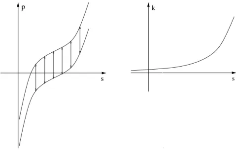
s p

s k

Figure 1: Illustration of the parameter functions. Left: the play-type hysteresis rela- tion. The curved lines correspond to p

_c

(s) + γ and p

_c

(s) − γ. For τ = 0, the pair (s, p) can move along the vertical lines (variable pressure at fixed saturation value).

Right: the positive permeability parameter k(s). In the analytical results, the coefficient functions p

_c

(s) and k(s) are extended to the real line s ∈ R .

Our main result is an existence theorem for system (1.1)–(1.2) of partial differ- ential equations. In the proof of this result we provide a Galerkin scheme, show the well-posedness of the scheme and a priori estimates, compactness results for the solu- tion sequence and the solution property for weak limits. One of the main analytical difficulties is to derive compactness of the sequence of saturations in L

²

(Ω × (0, T )), which is needed in order to take limits in the nonlinear terms. The equation allows to control time derivatives of the saturation and space derivatives of the pressure — but since there is no functional dependence, we cannot apply a Lions-Aubin lemma to conclude the compactness. We derive compactness via a careful analysis of the hysteresis relation with the compactness theorem of Riesz-Frechet-Kolmogorov.

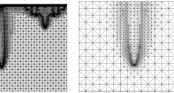
We include numerical results for the above model. In our calculations we use initial and boundary conditions that correspond to experiments regarding gravity fingering.

While the system without hysteresis cannot predict gravity fingers, our numerical results for the hysteresis system (1.1)–(1.2) show the appearance of gravity fingers.

1.1 Hysteresis models for the capillary pressure

Hysteresis is an important effect in porous media and it must be modelled correctly

for quantitative calculations and predictions. Additionally, even qualitative features

of flow in porous media depend on the capillary hysteresis. One example is the devel- opment of gravity fingers.

It is well known that the capillary pressure is different for imbibition and drainage processes, which means that a single function s 7→ p

_c

(s) is inappropriate for the description of processes where ∂

_t

s changes sign. Repeating imbibition and drainage procedures, one can explore a complex family of scanning curves between the two principle lines [11, 7]. Instead of prescribing a great number of scanning curves, it is desirable to develop a simple (thermodynamically consistent) model which includes hysteresis [15]. The most simple model is play-type hysteresis with vertical scanning curves. It is contained in (1.2) as the special case τ = 0. We use here the simplifying assumption that the imbibition curve is given by p

^im_c

(s) = p

_c

(s) + γ and the drainage curve by p

^dr_c

(s) = p

_c

(s) − γ. Note that p

_c

is the pressure of a non-wetting phase, therefore p

_c

is increasing.

The play type hysteresis has the disadvantage that all interior scanning curves are vertical and that, in particular, the pair (s, p) can move back and forth along the same line. These facts do not correspond to experiments. Nevertheless, if play type operators with different values of γ are averaged, then a Prandtl-Ishlinskii oper- ator replaces the play-type operator and scanning curves are no longer vertical. The Prandtl-Ishlinskii model was derived by rigorous homogenization from the play-type model in [22]. In this sense, imposing locally play-type hysteresis does not contradict experiments. The local use of the Prandtl-Ishlinskii operator is discussed also in [8].

The play type hysteresis is rate independent and models static hysteresis effects.

With different co-authors, Hassanizadeh included dynamic hysteresis effects with the parameter τ > 0 (in underlying models with and without static hysteresis). The full model appears as equation (11) in [8], if the above assumption is made on p

^im_c

and p

^dr_c

, and the wetting phase is not modelled, p

^w

≡ 0. The model was also used in [9], see their relations (4) and (5). Both contributions regard explicit one-dimensional solutions and thermodynamic considerations.

We emphasize that the play type hysteresis relation can (to a certain extend) be justified by an analysis of a pore-scale model. The relevant mechanism is the bottle- neck effect: the interface between wetting and non-wetting fluid in a single pore (with given contact angle) can move between narrow and wide regions of the pore. Such a change of the position of all the interfaces induces a macroscopic change of the pressure, but no macroscopic change of the saturation. In simple geometries, the argument can be made precise to provide a justification of the play-type hysteresis, see [20] and [21].

Regarding recently developed further extensions of the hysteresis model we mention [16] and the references therein.

1.2 Existence results for extended Richards equations

Even in the case without hysteresis, i.e. with an algebraic relation p = p

_c

(s) instead of (1.2), the Richards equation is an interesting mathematical object due to the possible degeneracies k(s) = 0 for some s and p

_c

(s

_k

) → ±∞ for s

_k

tending to critical saturation values. Existence results are obtained e.g. in [1] and [2], uniqueness is treated e.g. in [18] and [10], the physical outflow boundary conditions are treated e.g. in [3] and [23].

The relation (1.2), without the coupling to a partial differential equation, poses also

interesting questions regarding a functional analytic description and we refer to [28]

for the corresponding discussion. In both cases, τ = 0 (rate-independent) and τ > 0 (rate-dependent), the hysteresis relation may be considered as a functional relation s(t) = B(t, p|

_[0,t]

), where B maps the history of p to a value s(t), given initial values s

₀

. We emphasize that, even in the equilibrium situation ∂

t

s = 0, we cannot determine p(t) from s|

_[0,t]

. In this sense, the hysteresis relation cannot be inverted.

An existence result for the Richards equation with hysteresis was provided in [22]

in the case that the partial differential equation is linear, i.e. in the case that k(.) is not depending on s and that p

_c

(.) is an affine function. In this situation, it was possible to treat the case τ = 0. We note here that a positive parameter τ has a regularizing effect in the system and helps considerably in the analysis of the equations.

Existence results for the nonlinear system with hysteresis were obtained in [4]

and [5] under very general assumptions: coefficients can be degenerate, the hysteresis relation can be more general than play-type, and outflow boundary conditions are treated. Nevertheless, our problem is not covered by these contributions. In [4], the hysteresis relation s(t) = B(t, p|

_[0,t]

) is inverted (compare relation (3.7) of [4]), which is not possible in our model. In [5], another regularization of the equations was introduced, namely a time-convolution in the determination of the permeability coefficient k, which is not a common modelling approach.

1.3 Gravity fingering

Fingering is an effect that can occur when a more saturated layer is above a less saturated region of a porous medium. Under the influence of gravity, the fluid will move downward. For appropriately designed initial and boundary conditions, this downward flow happens in the form of fingers, i.e. the fluid moves mainly along long and thin subdomains of high saturation. The effect is known at least since the 1960’ies, recent studies are presented e.g. in [25, 6]. The phenomenon is similar to viscous fingering in Hele-Shaw cells, but it is more challenging in the sense that the standard models cannot explain the effect, see [14, 26]. Consequently, other models have been proposed, among them different “non-equilibrium Richards equations”, studied e.g. in [13, 17]. These models are related to a positive parameter τ .

The parameter τ > 0 introduces a form of dynamic hysteresis (we remark that the terminology is somewhat misleading, since the word hysteresis is usually reserved for rate independent processes). We include here both effects, dynamic hysteresis and static hysteresis. The static effects are modelled with the play-type relation and are certainly relevant in unsaturated porous media. One may even argue that the static hysteresis is the more important for the development of fingers: let us consider a point far away from the finger tip. The flow situation there is almost stationary. The fact that the finger does not widen at later stages must be a consequence of static hysteresis. Another argument that shows the importance of stationary hysteresis for fingering effects is the following instability result: planar wetting fronts under purely static hysteresis (i.e. τ = 0) are unstable, see [24].

Let us summarize the advantages of (1.1)–(1.2): the model includes static and

dynamic hysteresis, the static contribution is of play-type, which is the most simple

hysteresis model, it is consistent with thermodynamics and with experiments, and it

has a clear modelling foundation (bottle neck effect). The numerical results for this

model show the development of fingers in qualitative agreement with experiments. In

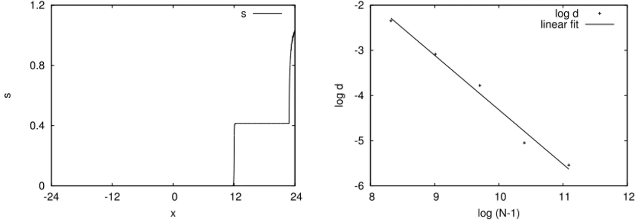
agreement with the one-dimensional analysis, the fingers develop a saturation maxi- mum at the tip (non-monotone saturation profile) only for positive values of τ .

2 Main result and preliminaries

2.1 Coefficient functions and main result

The unknowns in the porous media model (1.1)–(1.2) are pressure and saturation. A typical choice of function spaces is

p ∈ L

²

(0, T ; H

¹

(Ω, R )), s ∈ L

^∞

(0, T ; L

²

(Ω, R )). (2.1) We will actually achieve a solution with improved regularity, see Proposition 4.2. The solution depends on the initial values s

₀

∈ L

²

(Ω) for the saturation s, and on the boundary data g ∈ L

²

(0, T ; H

¹

(Ω)) for the pressure p; we will actually demand more regularity on these data. Furthermore, the solution depends on the coefficient functions p

_c

(x, s), k(x, s), and γ(x). We assume τ > 0 and for constants 0 < ρ < ρ

₁

, κ

₁

> 0, 0 < κ < κ

0

,

p

_c

, ∂

_s

p

_c

∈ C(Ω × R , R ), kp

_c

k

_Lip

≤ ρ

₁

, ∂

_s

p

_c

≥ ρ, (2.2) k, ∂

_s

k ∈ C(Ω × R , R ), κ

₀

≥ k(x, s) ≥ κ, |∂

_s

k(x, s)| ≤ κ

₁

, (2.3)

γ ∈ C

^0,1

(Ω, [0, ∞)). (2.4)

We emphasize that the Lipschitz continuity of p

_c

is assumed in x and s.

Remarks on the coefficient functions. The physically relevant range of satura- tion values is the interval [0, 1]. Since comparison principles are available for the above scalar parabolic problem, upon conditions on the coefficient function p

c

, the pressure boundary values g and the saturation initial values s

₀

, the saturation will only take values in [0, 1]. In this case, it is sufficient to consider p

_c

and k as functions on Ω×[0, 1].

The assumptions on the coeficient functions are used in the following steps. The bounds κ

₀

≥ k(x, s) ≥ κ > 0 in Lemma 3.1 and in the energy estimate of Proposition 3.2, the Lipschitz-continuity of k(x, ·) in Lemma 3.1, the Lipschitz-continuity of γ(·) in Lemma 3.3, the Lipschitz-continuity of p

c

in Lemma 3.1 and Proposition 3.2. The differentiability of k and p

_c

in s is only required for the higher order estimates in Section 4.

We treat here only the system with τ > 0. If one regularizes the multivalued sign-function to a single valued function Φ, then one may insert p from (1.2) into (1.1) to obtain an equation for s. Such an equation (usually with the linear operator ∆∂

_t

s on the right hand side) is called pseudo-parabolic. We do not use here the theory of pseudo-parabolic systems since we are interested in the multi-valued sign function (i.e.

we allow δ = 0 in the function Φ

^τ_δ

below).

The positivity assumption ∂

_s

p

_c

> ρ > 0 can actually be replaced by the much weaker assumption that there exists a primitive

P

_c

, ∂

_s

P

_c

∈ C(Ω × R , R ), P

_c

(x, s) ≥ 0, ∂

_s

P

_c

(x, s) = p

_c

(x, s). (2.5)

This means that we solve the pseudo-parabolic equation (τ > 0) even if the corre-

sponding parabolic equation has (partially) backward character.

Main Theorem. The aim of this contribution is to suggest and to analyze a spatial discretization of the above system and to show the convergence of the corresponding approximate solutions to a solution of the hysteresis problem.

Our analysis is – unfortunately – restricted to the case τ > 0. A positive coefficient τ has a regularizing effect in the equations and provides better a priori estimates on solutions. A positive time delay coefficient τ makes the problem rate dependent. Even though a rate independent system is more desirable in some applications, there are experiments that support the positivity of τ.

Theorem 2.1 (Approximation procedure and existence result). Let Ω ⊂ R

ⁿ

be a bounded polygonal domain, T > 0, and τ > 0. Let the coefficients p

_c

, k, γ satisfy (2.2)–

(2.4) and let initial and boundary data be given by s

₀

∈ L

²

(Ω) and g ∈ L

²

(0, T ; H

¹

(Ω)).

Then there exists a weak solution (s, p) of the hysteresis system (1.1)–(1.2) according to the solution concept of Definition 2.2.

The Galerkin discretization of the equations from Definition 2.4 provides approxi- mate solutions, depending on the grid size parameter h > 0 and, possibly, on a regu- larization parameter δ ≥ 0. In the limit h → 0 and δ → 0, the approximate solutions converge to a weak solution of the limit system.

Section 3 is devoted to the analysis of the discrete scheme. We show the solvability of the discrete system in Lemma 3.1 and provide a priori estimates of energy type in Proposition 3.2. The estimates control time derivatives of s and space derivatives of p. The compactness of the family of saturations relies on the hysteresis relation and is shown in Lemma 3.3. Finally, the weak limits of the approximate solutions are weak solutions to the hysteresis problem by Lemma 3.4.

Section 4 is devoted to uniform and to higher order estimates. Such estimates are not needed in the existence proof presented in Section 3. Nevertheless, we find it an interesting observation that, despite the nonlinearities in the equations, some higher order estimates are available (on arbitrary time intervals (0, T ) and not only locally).

These estimates guarantee, in particular, the strong convergence of the pressure ap- proximations ˜ p

^h

.

Section 5 shows results of an implementation of the scheme. We describe the performed time discretization and linearization and observe numerical convergence rates in an adaptive calculation. Our main interest is the application of the model to gravity fingers in unsaturated porous media. The numerical results show the fingering effect for small perturbations of the initial data. This confirms that the hysteresis model (1.1)–(1.2) can be used for the description of the fingering effect.

2.2 Solution concepts

We introduce a space discretization in order to define a sequence of approximate

solutions (s

^h

, p

^h

). Energy estimates provide integral bounds for ∂

_t

s

^h

and ∇p

^h

. We

select weakly convergent subsequences in the corresponding function spaces and find,

in the limit h → 0, weak solutions to the original problem. It will be one of the key

observations that s

^h

actually has a compactness property. It is worth noting here that

the hysteresis relation (which has p as an input and s as an output) does not allow to

conclude any compactness of the sequence p

^h

.

In the definition of the solution concept, the main point is to avoid nonlinear expressions in either p

^h

or ∂

_t

s

^h

. This prohibits, in particular, to use sign(∂

_t

s) or sign

⁻¹

(p − p

_c

(s)) in any variant. Our approach is to demand the linear relations explicitely in the distributional sense, and to encode non-linear relations with the help of a variational inequality.

Definition 2.2 (Weak solution). Let (s, p) be a pair of functions with

s ∈ L

^∞

(0, T ; L

²

(Ω)), ∂

_t

s ∈ L

²

(0, T ; L

²

(Ω)), (2.6)

p ∈ L

²

(0, T ; H

¹

(Ω)), (2.7)

satisfying, in the sense of traces, the initial condition s = s

₀

on Ω × {0} and the boundary condition p = g on ∂Ω × (0, T ). We call (s, p) a weak solution of the Richards equation with hysteresis when the following three conditions are satisfied.

1. The relation ∂

_t

s = ∇ · (k(s)[∇p + e

_n

]) holds in the sense of distributions.

2. The relation p(x, t) − p

_c

(x, s(x, t)) − τ ∂

_t

s(x, t) ∈ [−γ(x), γ(x)] holds for almost every (x, t).

3. There holds 0 ≥

Z

T 0

Z

Ω

(p

_c

(x, s(x, t)) − g(x, t)) ∂

_t

s(x, t) dx dt +

Z

T 0

Z

Ω

τ |∂

_t

s(x, t)|

²

+ γ(x) |∂

_t

s(x, t)| dx dt +

Z

T 0

Z

Ω

k(x, s(x, t)) (∇p(x, t) + e

_n

) ∇(p(x, t) − g(x, t)) dx dt.

(2.8)

Corollary 2.3. Weak solutions are also strong solutions in the following sense: the functions s, ∂

_t

s, p, and ∇p are in L

²

(Ω × (0, T )), equation (1.1) holds in the sense of distributions, (1.2) holds pointwise almost everywhere, the initial condition for s and the boundary condition for p are satisfied in the sense of traces. Theorem 2.1 therefore provides the existence of strong solutions to the hysteresis system.

Proof. We only have to show that (1.2) holds almost everywhere. For weak solutions, the distribution ∂

_t

s = ∇·(k(s)[∇p+e

_n

]) is actually an L

²

(Ω×(0, T )) function, hence we can perform an integration by parts in the third integral of (2.8). Then the inequality (2.8) simplifies to

0 ≥ Z

T

0

Z

Ω

[p

_c

(x, s(x, t)) − p(x, t)]∂

_t

s(x, t) dx dt +

Z

T 0

Z

Ω

τ |∂

_t

s(x, t)|

²

+ γ(x) |∂

_t

s(x, t)| dx dt.

We write this as

Z

T 0

Z

Ω

γ |∂

_t

s| ≤ Z

T

0

Z

Ω

[p − p

_c

(., s) − τ ∂

_t

s]∂

_t

s.

By the second property of weak solutions, the integrand on the right hand side satisfies [p − p

_c

(., s) − τ ∂

_t

s]∂

_t

s ≤ γ|∂

_t

s| almost everywhere, hence it is (pointwise) less or equal than the integrand on the left hand side. The inequality of the integrals therefore implies that the integrands coincide almost everywhere, i.e. [p − p

c

(., s) − τ ∂

t

s]∂

t

s = γ |∂

_t

s| almost everywhere. In points (x, t) with ∂

_t

s(x, t) 6= 0 we conclude p(x, t) − p

_c

(x, s(x, t)) −τ ∂

_t

s(x, t) ∈ γ(x) sign(∂

_t

s(x, t)). Instead, in points (x, t) with ∂

_t

s(x, t) = 0, the relation p(x, t) − p

c

(x, s(x, t)) − τ ∂

t

s(x, t) ∈ γ(x) sign(0) holds by the second property of weak solutions.

2.3 Regularization and discretization

We recall that three positive (and possibly small) physical parameters appear in the equations: the number κ > 0 is a lower bound for the permeability, ρ > 0 is a lower bound for the slope of p

_c

, and τ > 0 is the time delay parameter. We introduce two further positive parameters, which allow to introduce a well-posed approximate prob- lem: a regularization parameter for the sign-function, δ > 0, and a space-discretization parameter h > 0.

In the case τ = 0, the play-type relation (1.2) can be written with the function Φ

⁰₀

(σ) := γ sign(σ) as p ∈ p

_c

(s) + Φ

⁰₀

(∂

_t

s). For the general case τ ≥ 0 we introduce Φ

^τ₀

:= Φ

⁰₀

+ τ id, i.e.

Φ

^τ₀

(σ) :=



 

 

[−γ(x), γ(x)] for σ = 0 γ(x) + τ σ for σ > 0

−γ(x) + τ σ for σ < 0

(2.9)

This function is multivalued. The inverse function is denoted by Ψ

^τ₀

:= (Φ

^τ₀

)

⁻¹

, it is multivalued for τ = 0. For positive τ, the function Ψ

^τ₀

is single-valued with maximal slope τ

⁻¹

. In this sense, a positive parameter τ introduces a regularization.

Regularization. In numerical schemes, it can be advantageous to introduce another regularization. With a parameter δ > 0, we introduce the regularized functions

Φ

^τ_δ

(σ) :=



 



 



γ(x)

δ

+ τ

σ for σ ∈ [−δ, δ]

γ(x) + τ σ for σ > δ

−γ(x) + τ σ for σ < −δ

(2.10)

such that Φ

^τ_δ

(±δ) = γ(x) ± τ δ = Φ

^τ₀

(±δ) and such that the relation Φ

^τ_δ

= Φ

⁰_δ

+ τ id remains valid. The inverse of Φ

^τ_δ

is denoted as Ψ

^τ_δ

. For τ, δ > 0, both functions Φ

^τ_δ

and Ψ

^τ_δ

are single-valued, globally Lipschitz continuous, and strictly monotonically increasing. In the above notation, we suppressed everywhere the dependence on the parameter γ ≥ 0.

Spatial discretization. We now discretize the spatial domain Ω in order to con-

struct a Galerkin scheme. We assume that we are given a triangulation T

_h

of the

polygonal domain Ω, where the triangles A ∈ T

_h

satisfy uniform bounds on the angles

and where the diameter of the largest triangle is bounded by h > 0. To every triangle

A ∈ T

h

we associate a corner x ∈ Ω

h

, where Ω

h

is a subset of N corners. This map defines a projection X

^h

: Ω → Ω

_h

= {x

₁

, . . . , x

_N

}, X

^h

: A

_k

3 x 7→ x

_k

. The map X

^h

additionally defines an invertible map which identifies R

^N

with piecewise constant functions,

J : R

^N

≡ {f : Ω

_h

→ R } → {f : Ω → R piecewise constant} =: P

₀

(Ω, T

_h

), (2.11) by (J f )(x) = f(X

^h

(x)). We will furthermore use the L

²

-orthogonal projection P :=

P

_h

: L

²

(Ω) → L

²

(Ω) to the space of piecewise constant functions P

₀

(Ω, T

_h

). In ad- dition, we discretize the parameter γ as γ

^h

:= J(γ|

_Ωh

). To this piecewise constant parameter function γ

^h

we denote the corresponding regularization of γ

^h

sign + τ id by Φ

^τ_δ,h

(σ) = Φ

^τ_δ,h

(σ; x) and its inverse by Ψ

^τ_δ,h

(z) = Φ

^τ_δ,h

(z; x). We are now in a position to define our Galerkin scheme.

Definition 2.4 (Galerkin scheme). We consider the following system of ordinary dif- ferential equations for p

^h

: Ω × [0, T ] → R and s

^h

: Ω × [0, T ] → R piecewise constant.

∂

t

s

^h

(x

k

, t) = −Ψ

^τ_δ,h

(p

c

(x

k

, s

^h

) − p

^h

(x

k

, t)) ∀x

k

∈ Ω

h

(2.12)

s

^h

(., 0) = P

_h

s

₀

, (2.13)

where we suppressed the explicit dependence of Ψ

^τ_δ,h

on x

_k

. The pressure p

^h

is recon- structed from s

^h

as follows. We solve for p ˜

^h

(., t) : Ω → R the elliptic problem

∇ · k(x, s

^h

)(∇ p ˜

^h

+ e

_n

)

= −Ψ

^τ_δ,h

p

_c

(x, s

^h

) − P

_h

p ˜

^h

in Ω (2.14)

˜

p

^h

(·, t) = g(·, t) on ∂Ω, (2.15) for all t ∈ [0, T ], and set p

^h

= P

_h

p ˜

^h

.

For later reference we note that the ordinary differential equation (2.12) can be written also with the (for δ = 0 multivalued) functions Φ

⁰_δ,h

and Φ

^τ_δ,h

as

Φ

^τ_δ,h

(∂

_t

s

^h

(x

_k

, t)) = Φ

⁰_δ,h

(∂

_t

s

^h

(x

_k

, t)) + τ ∂

_t

s

^h

(x

_k

, t) 3 p

^h

(x

_k

, t) − p

_c

(x

_k

, s

^h

). (2.16)

3 Well-posedness, uniform estimates, compactness, and limit procedure

3.1 Well-posedness of the Galerkin scheme

We have to show that the elliptic equation (2.14) with boundary condition (2.15) defines a Lipschitz-continuous map s

^h

7→ p

^h

= P

_h

p ˜

^h

. Once this is shown, the Galerkin scheme is reduced to the ordinary differential equation (2.12). The subsequent lemma performs this analysis of (2.14), where we write u + g instead of ˜ p and denote test- functions by v. Our aim is to solve A

_h

u = 0.

Lemma 3.1 (Local existence result for the discrete system). For τ > 0, h > 0 and s ∈ L

^∞

(Ω) piecewise constant we define two nonlinear operators A

0

, A

h

: H

₀¹

(Ω) → H

⁻¹

(Ω) by

hA

_h

u, ϕi :=

k x, s

(∇u + ∇g + e

_n

), ∇ϕ

L²(Ω)

−

Ψ

^τ_δ,h

p

_c

(x, s) − P

_h

(u + g) , ϕ

L²(Ω)

hA

₀

u, ϕi :=

k x, s

(∇u + ∇g + e

_n

), ∇ϕ

L²(Ω)

−

Ψ

^τ_δ,h

p

_c

(x, s) − (u + g) , ϕ

L²(Ω)

for all ϕ ∈ H

₀¹

(Ω), where P

h

ist the projection to piecewise constant functions, the operator A

₀

is the operator A

_h

without the projection. We suppress the s-dependence of the operators A

₀

= A

^s₀

and A

_h

= A

^s_h

if it is not relevant. There exists h

₀

= h

₀

(τ, g) > 0 such that the following holds:

1. The operator A

0

is monotone, coercive and continuous on finite dimensional subspaces. There exists a continuous solution operator A

⁻¹₀

: H

⁻¹

(Ω) → H

₀¹

(Ω).

2. For every f ∈ L

²

(Ω) and every h ∈ [0, h

₀

] there exists a unique u ∈ H

₀¹

(Ω) satisfying A

_h

u = f. The following inequality holds:

kuk

_H¹_(Ω)

≤ C(s, g) 1 + kfk

_L²_(Ω)

, (3.1)

where the constant C depends on ksk

_L²_(Ω)

and kgk

_L²_(Ω)

and not on h.

3. For every h ∈ [0, h

₀

] the map L

^∞

(Ω) 3 s 7→ (A

^s_h

)

⁻¹

(0) ∈ H

₀¹

(Ω) is locally Lipschitz continuous.

Item 3 of Lemma 3.1 shows that the the elliptic equation (2.14)–(2.15) defines a Lipschitz continuous map s

^h

(t) 7→ p

^h

(t) = P

_h

(u + g). In particular, (2.12)–(2.13) of Definition 2.4 describes a system of ordinary differential equtions. We conclude that for δ ≥ 0 and sufficiently small h > 0 there exists a unique local solution (p

^h

, s

^h

) to the Galerkin scheme of Definition 2.4.

Proof. Item 1. For the monotonicity of A

0

we calculate hA

₀

u − A

₀

v, u − vi =

k x, s

(∇u − ∇v), ∇u − ∇v

L²(Ω)

−

Ψ

^τ_δ,h

p

c

(x, s) − (u + g)

− Ψ

^τ_δ,h

p

c

(x, s) − (v + g)

, u − v

L²(Ω)

≥ κh∇(u − v), ∇(u − v)i

_L²_(Ω)

.

We exploited here the lower bound k ≥ κ and the monotonicity of Ψ

^τ_δ,h

(·). The right hand side is non-negative and we conclude the (strict) monotonicity of A

₀

. A similar calculation, using additionally the Poincar´ e inequality, yields the coerciveness of A

₀

.

hA

₀

u, ui ≥C

₁

κkuk

²_H1(Ω)

− C

₂

(τ, s, g)kuk

_H¹_(Ω)

,

where C

₁

> 0 depends on the Poincar´ e constant and C

₂

(τ, s, g) ∈ R is independent of h. We conclude

hA

₀

u, ui

kuk

_H¹_(Ω)

→ ∞ for kuk

_H¹_(Ω)

→ ∞,

and thus the coercivity of A

₀

. The continuity of A

₀

on finite dimensional subspaces fol- lows from the continuity of Ψ

^τ_δ

. The theory of monotone operators yields the existence of a unique solution u to A

0

u = f .

The continuity of the solution operator A

⁻¹₀

is shown with a similar calculation: We

consider A

₀

u = f

₁

and A

₀

v = f

₂

and calculate as for the monotonicity ku − v k

_H¹_(Ω)

≤

Ckf

₁

− f

₂

k

_H⁻¹_(Ω)

.

Item 2. We now prove inequality (3.1) for solutions of A

h

u = f. We write the relation hA

_h

u, ui = hf, ui

_L²_(Ω)

as

Z

Ω

k(x, s) (∇u + ∇g + e

_n

) ∇u dx − Z

Ω

Ψ

^τ_δ,h

p

_c

(x, s) − P

_h

(u + g)

u dx = Z

Ω

f u dx.

The first term on the left hand side is estimated in the standard way as Z

Ω

k(x, s) (∇u + ∇g + e

_n

) ∇u dx ≥ C

₁

κkuk

²_H1(Ω)

− C

₂

(κ

₀

, g)k∇uk

_L²_(Ω)

,

where C

1

> 0 depends on the Poincar´ e constant and C

2

(κ

0

, g) ∈ R depends on the uniform bound k ≤ κ

₀

. For the second term we calculate

− Z

Ω

Ψ

^τ_δ,h

p

c

(x, s) − P

h

(u + g) u dx

= − Z

Ω

Ψ

^τ_δ,h

p

_c

(x, s) − P

_h

(u + g)

(P

_h

u + (u − P

_h

u)) dx

= Z

Ω

Ψ

^τ_δ,h

p

_c

(x, s) − P

_h

g

− Ψ

^τ_δ,h

p

_c

(x, s) − P

_h

(u + g)

P

_h

u dx

− Z

Ω

Ψ

^τ_δ,h

p

_c

(x, s) − P

_h

g

P

_h

u dx − Z

Ω

Ψ

^τ_δ,h

p

_c

(x, s) − P

_h

(u + g)

(u − P

_h

u) dx

≥ − Z

Ω

Ψ

^τ_δ,h

p

_c

(x, s) − P

_h

g

P

_h

u dx − Z

Ω

Ψ

^τ_δ,h

p

_c

(x, s) − P

_h

(u + g)

(u − P

_h

u) dx

≥ −C(τ, g, s)kP

_h

uk

_L²_(Ω)

− 1

τ C(s, g) + kP

_h

uk

_L²_(Ω)

ku − P

_h

uk

_L²_(Ω)

≥ −C(τ, g, s)kuk

_L²_(Ω)

− 1

τ C(s, g) + kuk

_H¹_(Ω)

Chkuk

_H¹_(Ω)

,

where we exploited the monotonicity of Ψ

^τ_δ,h

, the Lipschitz bound for p

_c

(x, .), and for the projection P

_h

the facts kP

_h

uk

_L²_(Ω)

≤ kuk

_L²_(Ω)

and ku − P

_h

uk

_L²_(Ω)

≤ Chkuk

_H¹_(Ω)

. For h sufficiently small (depending on τ > 0), we can then absorb the negative quadratic term −

^Ch_τ

kuk

²_H1(Ω)

into the positive term C

₁

κkuk

²_H1(Ω)

. Similarly, linear terms in kuk

_H¹_(Ω)

can be absorbed. Applying the H¨ older inequality to R

Ω

f u dx pro- vides the claimed estimate (3.1).

In our next step we prove the existence of a solution u to A

_h

u = f for h > 0.

We use that for h = 0 a unique solution exists and apply the Schauder fixed point Theorem to the operator T , which we define as

T (u) : = A

⁻¹₀

(f − A

_h

(u) + A

₀

(u))

= A

⁻¹₀

f + Ψ

^τ_δ,h

p

_c

(x, s) − (u + g)

− Ψ

^τ_δ,h

p

_c

(x, s) − P

_h

(u + g)

We note that a fixed point of T solves A

_h

u = f , which is the desired relation. In order to apply the Schauder fixed point Theorem we show: (i) The operator T is compact.

(ii) There exists R > 0 such that T : H

¹

(Ω) ⊃ B

R

(0) → B

R

(0), where B

R

(0) denotes the ball with radius R with respect to the H

¹

(Ω)-norm.

Concerning (i): The embedding id : H

¹

(Ω) → L

²

(Ω) is compact and the operator

T is continuous as an operator from L

²

(Ω) to H

¹

(Ω). Thus the composition T ◦ id :

H

¹

(Ω) → H

¹

(Ω) is compact.

Concerning (ii): Exploiting estimate (3.1) for A

0

we calculate for u with kuk

_H¹

≤ R kT (u)k

_H¹_(Ω)

≤ C(s) 1 +

f + Ψ

^τ_δ,h

(p

_c

(x, s) − (u + g)) − Ψ

^τ_δ,h

(p

_c

(x, s) − P

_h

(u + g))

L²(Ω)

≤ C(s)

1 + kfk

_L²_(Ω)

+ 1

τ kP

_h

(u + g) − (u + g)k

_L2(Ω)

≤ C(s)

C(f) + 1

τ Ch kuk

_H¹_(Ω)

+ kgk

_H¹_(Ω)

≤ C(s)

C(f, g, τ ) + Ch τ R

≤ R for R > 0 sufficiently large and h > 0 sufficiently small, depending on τ and s.

Item 3. We now show the local Lipschitz continuity of the map s 7→ (A

^s_h

)

⁻¹

(0) and, in particular, that the map s 7→ (A

^s_h

)

⁻¹

(0) is well defined. We consider two discrete saturation variables s

1

, s

2

∈ L

^∞

(Ω). Since we are interested in a local Lipschitz property, we assume the boundedness ks

₁

k

_L^∞

, ks

₂

k

_L^∞

≤ R for some R > 0. We consider the corresponding operators A

^s_h¹

, A

^s_h²

and two solutions u

₁

and u

₂

of A

^s_h¹

u

₁

= 0 and A

^s_h²

u

2

= 0. Then

0 = hA

^s_h¹

u

₁

− A

^s_h²

u

₂

, u

₁

− u

₂

i

=

k x, s

₁

(∇u

₁

+ ∇g + e

_n

) − k x, s

₂

(∇u

₂

+ ∇g + e

_n

), ∇u

₁

− ∇u

₂

L²(Ω)

−

Ψ

^τ_δ,h

p

_c

(x, s

₁

) − P

_h

(u

₁

+ g)

− Ψ

^τ_δ,h

p

_c

(x, s

₂

) − P

_h

(u

₂

+ g)

, u

₁

− u

₂

L²(Ω)

=: Z

1

+ Z

2

We treat the term Z

₁

as follows Z

1

=

k x, s

1

− k x, s

2

(∇g + e

n

), ∇u

1

− ∇u

2

L²(Ω)

+ hk(x, s

₁

) (∇u

₁

− ∇u

₂

) , ∇u

₁

− ∇u

₂

i

_L2(Ω)

+ h(k(x, s

₁

) − k(x, s

₂

)) ∇u

₂

, ∇u

₁

− ∇u

₂

i

_L2(Ω)

≥ −C(g)ks

₁

− s

₂

k

_L^∞_(Ω)

k∇u

₁

− ∇u

₂

k

_L²_(Ω)

+ κk∇u

1

− ∇u

2

k

²_L2(Ω)

− κ

1

ks

1

− s

2

k

_L^∞_(Ω)

k∇u

2

k

_L²_(Ω)

k∇u

1

− ∇u

2

k

_L²_(Ω)

≥ Cκku

₁

− u

₂

k

²_H1(Ω)

− C(R, g)ks

₁

− s

₂

k

_L^∞_(Ω)

k∇u

₁

− ∇u

₂

k

_L²_(Ω)

,

where we have used the Poincar´ e inequality, the Lipschitz constant κ

₁

of k(x, ·) and the a priori estimate (3.1) for u

2

. The lower order term Z

2

can be estimated as follows Z

₂

= −

Ψ

^τ_δ,h

p

_c

(x, s

₁

) − P

_h

(u

₁

+ g)

− Ψ

^τ_δ,h

p

_c

(x, s

₂

) − P

_h

(u

₂

+ g) , (id − P

_h

)(u

₁

− u

₂

)i

_L2(Ω)

−

Ψ

^τ_δ,h

p

_c

(x, s

₁

) − P

_h

(u

₁

+ g)

− Ψ

^τ_δ,h

p

_c

(x, s

₂

) − P

_h

(u

₂

+ g )

, P

_h

(u

₁

− u

₂

)

L²(Ω)

≥ − 1

τ kp

c

(x, s

1

) − P

h

u

1

− p

c

(x, s

2

) + P

h

u

2

k

_L²_(Ω)

k(id − P

h

)(u

1

− u

2

)k

_L²_(Ω)

−

Ψ

^τ_δ,h

p

_c

(x, s

₁

) − P

_h

(u

₁

+ g)

− Ψ

^τ_δ,h

p

_c

(x, s

₁

) − P

_h

(u

₂

+ g )

, P

_h

(u

₁

− u

₂

)

L²(Ω)

−

Ψ

^τ_δ,h

p

_c

(x, s

₁

) − P

_h

(u

₂

+ g)

− Ψ

^τ_δ,h

p

_c

(x, s

₂

) − P

_h

(u

₂

+ g )

, P

_h

(u

₁

− u

₂

)

L²(Ω)

≥ − 1

τ Cρ

₁

ks

₁

− s

₂

k

_L^∞_(Ω)

+ kP

_h

u

₁

− P

_h

u

₂

k

_L²_(Ω)

Chku

₁

− u

₂

k

_H¹_(Ω)

−

Ψ

^τ_δ,h

p

_c

(x, s

₁

) − P

_h

(u

₂

+ g)

− Ψ

^τ_δ,h

p

_c

(x, s

₂

) − P

_h

(u

₂

+ g )

, P

_h

(u

₁

− u

₂

)

L²(Ω)

≥ −Ch 1

τ ks

₁

− s

₂

k

_L^∞_(Ω)

+ ku

₁

− u

₂

k

_H¹_(Ω)

ku

₁

− u

₂

k

_H¹_(Ω)

− 1

τ Cks

₁

− s

₂

k

_L^∞_(Ω)

ku

₁

− u

₂

k

_H¹_(Ω)

,

where we used the monotonicity of Ψ

^τ_δ,h

and the Lipschitz continuity of Ψ

^τ_δ,h

and p

_c

(x, ·).

For sufficiently small h > 0 the quadratic negative term −

^Ch_τ

ku

₁

− u

₂

k

²_H1(Ω)

can be absorbed into the positive term Cκku

1

− u

2

k

²_H1(Ω)

of Z

1

. We thus conclude from Z

₁

+ Z

₂

= 0 the estimate

ku

1

− u

2

k

²_H1(Ω)

≤ C(R, g, τ)ks

1

− s

2

k

L^∞(Ω)

ku

1

− u

2

k

_H¹_(Ω)

,

and hence the local Lipschitz continuity of the map s 7→ (A

^s_h

)

⁻¹

(0).

3.2 Energy estimates

Our next aim is to derive for s

^h

estimates that do not depend on the regularization parameters h and δ. One consequence of the subsequent proposition is that we can extend the local solutions of the Galerkin scheme to the whole interval [0, T ].

Proposition 3.2 (Energy estimates and global solutions). Every solution p ˜

^h

, s

^h

to the scheme of Definition 2.4 satisfies the uniform bounds

k˜ p

^h

k

²_L2(0,T;H¹(Ω))

+ k∂

_t

s

^h

k

²_L2(0,T;L²(Ω))

≤ C, (3.2) where the constant C depends on initial and boundary data, on κ, τ , κ

₀

, and ρ

₁

, but it is independent of h > 0 and δ ≥ 0.

Proof. We start by writing the Galerkin evolution equation in a form that is similar to the original formulation. We apply the operator J (identification with piecewise constant functions) to (2.12) and use (2.14) to write

∂

t

s

^h

− ∇ · k(x, s

^h

)(∇ p ˜

^h

+ e

n

)

= −JΨ

^τ_δ,h

(p

_c

(x, s

^h

) − p

^h

) + Ψ

^τ_δ,h

p

_c

(x, s

^h

) − p

^h

. (3.3)

Multiplication with ˜ p

^h

− g and integration over Ω yields Z

Ω

∂

t

s

^h

p ˜

^h

− g dx +

Z

Ω

k(x, s

^h

)(∇˜ p

^h

+ e

n

) ∇˜ p

^h

− ∇g dx

= − Z

Ω

J Ψ

^τ_δ,h

(p

_c

(x, s

^h

) − p

^h

) − Ψ

^τ_δ,h

p

_c

(x, s

^h

) − p

^h

˜ p

^h

− g

dx.

(3.4)

We will conclude the a priori energy estimate (3.2) from equation (3.4). We will

identify several positive terms on the left hand side, the right hand side will turn out

to be small.

In order to treat the time derivative in the first integral, we use the hysteresis differential equation in the form (2.16) and apply the operator J,

JΦ

⁰_δ,h

(∂

_t

s

^h

(x, t)) + τ ∂

_t

s

^h

(x, t) 3 p

^h

(x, t) − J p

_c

(x, s

^h

). (3.5) Using P

_h

p ˜

^h

= p

^h

and the orthogonality

∂

_t

s

^h

, p ˜

^h

L²

=

∂

_t

s

^h

, p

^h

L²

, we find, exploiting the monotonicity of Φ

⁰_δ,h

,

Z

Ω

∂

_t

s

^h

p ˜

^h

dx ∈ Z

Ω

∂

_t

s

^h

JΦ

⁰_δ,h

(∂

_t

s

^h

) + τ ∂

_t

s

^h

+ J p

_c

(x, s

^h

) dx

≥ τk∂

_t

s

^h

k

²_L2(Ω)

+ Z

Ω

∂

_t

s

^h

J p

_c

(x, s

^h

) dx.

In order to analyze the last integral we use a primitive P

_c

(x, ·) of the function p

_c

(x, ·), i.e. ∂

_s

P

_c

(x, s) = p

_c

(x, s). Due to ρ > 0 (or by using (2.5)), we can assume the non-negativity of P

_c

. With this primitive, we calculate

Z

Ω

∂

t

s

^h

J p

c

(x, s

^h

) dx = Z

Ω

J d

dt P

c

(x, s

^h

)

dx = ∂

t

Z

Ω

J P

c

(x, s

^h

) dx.

For the second term on the left hand side of (3.4) we calculate Z

Ω

k(x, s

^h

)(∇ p ˜

^h

+ e

_n

)∇ p ˜

^h

dx ≥ κk∇ p ˜

^h

k

²_L2(Ω)

− Ck∇ p ˜

^h

k

_L²_(Ω)

≥ κ

2 k∇ p ˜

^h

k

²_L2(Ω)

− 2C

²

κ , where C depends on κ

₀

, the uniform bound for k. The terms on the left hand side of (3.4) containing the boundary data g are treated as follows.

Z

Ω

∂

_t

s

^h

g dx

+ Z

Ω

k(x, s

^h

)(∇ p ˜

^h

+ e

_n

)∇g dx

≤ τ

2 k∂

_t

s

^h

k

²_L2(Ω)

+ 2

τ kgk

²_L2(Ω)

+ κ

4 k∇ p ˜

^h

k

²_L2(Ω)

+ C

κ k∇gk

²_L2(Ω)

+ Ck∇gk

_L²_(Ω)

= τ

2 k∂

_t

s

^h

k

²_L2(Ω)

+ κ

4 k∇˜ p

^h

k

²_L2(Ω)

+ C(g) 1 κ ,

where the constant C depends on the uniform bound κ

₀

of k. Consequently, the s

^h

, p ˜

^h

-dependent terms can be absorbed.

We finally treat the error term on the right hand side of (3.4). We consider an arbitrary point x in a triangle with associated vertex x

_k

= X

^h

(x).

J Ψ

^τ_δ,h

(p

_c

(·, s

^h

) − p

^h

) − Ψ

^τ_δ,h

p

_c

(·, s

^h

) − p

^h

(x)

=

Ψ

^τ_δ,h

(p

_c

(x

_k

, s

^h

) − p

^h

) − Ψ

^τ_δ,h

p

_c

(x, s

^h

) − p

^h

≤ 1 τ

(p

_c

(x

_k

, s

^h

) − p

_c

(x, s

^h

) ≤ 1

τ ρ

₁

h,

where we exploit the Lipschitz continuity of Ψ

^τ_δ,h

and the Lipschitz continuity of p

c

in x. With this pointwise estimate, equation (3.4) yields

κ

4 k∇ p ˜

^h

k

²_L2(Ω)

+ τ

2 k∂

_t

s

^h

k

²_L2(Ω)

+ ∂

t

Z

Ω

J P

c

(x, s

^h

) dx

≤ 2C

²

+ C(g)

κ + ρ

₁

h

τ k p ˜

^h

k

_L²_(Ω)

+ kg k

_L²_(Ω)

.

Using the Poincar´ e inequality, the last product can also be absorbed. An integration

over (0, T ) provides estimate (3.2).

3.3 Bounds and compactness from the hysteresis relation

Lemma 3.3 (Regularity and compactness from the hysteresis relation). Let s

^h

and

˜

p

^h

satisfy the ordinary differential equation of the hysteresis relation (2.12), i.e.

∂

_t

s

^h

(x

_k

, t) = −Ψ

^τ_δ,h

(p

_c

(x

_k

, s

^h

) − p

^h

(x

_k

, t)) ∀x

_k

∈ Ω

_h

s

^h

(x

_k

, 0) = P

_h

s

₀

(x

_k

)

for p

^h

= P

_h

p ˜

^h

. Then, for every q ∈ [1, ∞] and s

₀

∈ L

^q

(Ω), we find the estimate k∂

t

s

^h

k

_L²_(0,T;L^q_(Ω))

+ ks

^h

k

_L²_(0,T;L^q_(Ω))

≤ Ck˜ p

^h

k

_L²_(0,T;L^q_(Ω))

, (3.6) where the constant C does not depend on h and δ.

Let additionally the following estimate hold with C independent of h and δ,

k˜ p

^h

k

_L²_(0,T;H¹_(Ω))

≤ C. (3.7) Then the family s

^h

is pre-compact in the space L

²

(Ω × (0, T )).

Proof. We recall the following characterization of the L

²

-orthogonal projection P = P

_h

onto piecewise constant functions with the help of averages. For an arbitrary L

²

- function ˜ u, the projection u = P u ˜ satisfies

u(x) = 1

|A

_k

| Z

Ak

˜

u(x) dx ∀x ∈ A

_k

, (3.8)

for each simplex A

k

∈ T

h

. This can easily be verified from the fact that u minimizes the L

²

-distance to ˜ u. A consequence of this characterization of P and Jensens’s inequality is the estimate

kP uk ˜

^q_Lq(Ω)

= X

k

Z

Ak

|P u| ˜

^q

= X

k

|A

_k

| − Z

Ak

− Z

Ak

˜ u

q

≤ X

k

|A

_k

| − Z

Ak

|˜ u|

^q

= k˜ uk

^q_Lq(Ω)

. In particular, the pressure functions satisfy kp

^h

(t)k

_L^q_(Ω)

≤ k˜ p

^h

(t)k

_L^q_(Ω)

.

Estimates. We now study solutions s

^h

of the hysteresis relation. We start with an arbitrary point x

k

∈ Ω

h

and note that

∂

_t

|s

^h

(x

_k

, t)| ≤

Ψ

^τ_δ,h

(p

_c

(x

_k

, s

^h

) − p

^h

(x

_k

, t))

≤ C|s

^h

(x

_k

, t)| + C|p

^h

(x

_k

, t)|.

An application of Gronwalls inequality yields pointwise, with C = C(τ, T ) independent of h and δ, the bound |s

^h

(x

_k

, t)| ≤ C|p

^h

(x

_k

, t)|. Using a second time the evolution equation, we also find an estimate for the time derivative,

|∂

t

s

^h

(x

k

, t)| + |s

^h

(x

k

, t)| ≤ C|p

^h

(x

k

, t)|.

Taking the q-th power and adding the inequalities over the triangles yields k∂

_t

s

^h

(t)k

^q_Lq(Ω)

+ ks

^h

(t)k

^q_Lq(Ω)

≤ C X

k

|A

_h,k

|

p

^h

(x

_k

, t))

q

= Ckp

^h

k

^q_Lq(Ω)

≤ Ck˜ p

^h

k

^q_Lq(Ω)

.

Taking an appropriate power and integrating over time, this provides the desired

estimate (3.6).

Compactness. Estimate (3.6) allows to conclude from the bound (3.7) for the pressures the boundedness of a time derivative of the saturation,

k∂

_t

s

^h

k

_L²_(0,T;L²_(Ω))

≤ Ck˜ p

^h

k

_L²_(0,T;L²_(Ω))

≤ C. (3.9) We remark that, for the Galerkin scheme used here, this time regularity of s was already a direct consequence of the energy estimate. It remains to transfer the spa- tial regularity of the pressures from (3.7) to the saturation in order to conclude the compactness rom the compactness theorem of Riesz-Frechet-Kolmogorov.

Step 1. Spatial shifts of the pressure inputs. In the following we will consider functions f ∈ L

²

(Ω) also as functions f ∈ L

²

( R

ⁿ

) by the trivial extension. For such functions in the (spatial) domain R

ⁿ

and an arbitrary vector y ∈ R

ⁿ

we introduce the shift operator L

_y

: L

²

( R

ⁿ

) → L

²

( R

ⁿ

), f 7→ L

_y

f through L

_y

f (x) = f (x − y).

A bounded family f

^h

∈ H

¹

(Ω), indexed with h, satisfies sup

_h

kL

_y

f

^h

−f

^h

k

_L²_(Rⁿ₎

→ 0 for y → 0. This can be concluded either in an abstract way via the characterization of compact subsets of L

²

( R

ⁿ

) through the Riesz-Frechet-Kolmogorov theorem. The more direct proof is to write f (x − y) − f (x) = R

1

0

∇f(x − ty) · y dt, and to integrate over x. Concerning the boundary layer where f(x) 6= 0 is compared with the value 0 of the extended function, we note that kf

^h

k

_L^q_(Rⁿ₎

is bounded for some q > 2, hence the boundary layer gives only a small contribution for small |y|. In this way, we also achieve an estimate kL

_y

f

^h

− f

^h

k

²_L2(Rⁿ)

≤ C|y|

^α

kf

^h

k

²_H1(Ω)

for some fixed α > 0. This estimate remains valid after an integration over (0, T ) and we find

sup

h

kL

_y

p ˜

^h

− p ˜

^h

k

_L²_(0,T;L²_(Rⁿ₎₎

→ 0 for |y| → 0. (3.10) In the following, we write only k.k

_L²_L²

in order to indicate the above norm.

Step 2. Spatial shifts of projected pressures. We next consider the projected pres- sures p

^h

= P p ˜

^h

with the aim to show

sup

h

kL

_y

p

^h

− p

^h

k

_L²_L²

→ 0 for |y| → 0. (3.11) We first study the case that h is large compared to |y|. We claim that

sup

h≥|y|^1/2

kL

_y

p

^h

− p

^h

k

_L²_L²

→ 0 for |y| → 0. (3.12) In this situation we consider a piecewise constant function and compare this function with its (slightly) shifted version. We use the triangles A

_k

and the selected points x

_k

∈ A ¯

k

corresponding to A

k

, with k in a finite index set. Since the function (L

y

p

^h

− p

^h

)|

A_k

is non-vanishing only on a set of measure C|y|h

ⁿ⁻¹

, we can calculate, using that all triangles have comparable size,

kL

_y

p

^h

− p

^h

k

²_L2L²

= Z

T

0

( X

k

Z

Ak

|p

^h

(x − y) − p

^h

(x)|

²

)

dt

≤ C Z

T

0

(

|y|h

ⁿ⁻¹

X

k

|p

^h

(x

k

)|

²

)

dt ≤ C |y|

h Z

T

0

( X

k

h

ⁿ

|p

^h

(x

k

)|

²

)

dt

≤ C |y|

h kp

^h

k

²_L2L²

.