Wave Solutions of Evolution Equations
Wolf-Jürgen Beyn1
Department of Mathematics Bielefeld University
33501 Bielefeld Germany
Denny Otten2
Department of Mathematics Bielefeld University
33501 Bielefeld Germany
Date: December 20, 2016 Contents
1. Introduction 2
2. Examples and basic principles 3
2.1. Travelling wave solutions 3
2.2. Examples from linear PDEs 5
2.3. Travelling waves in nonlinear parabolic PDEs 9 2.4. Phase plane analysis of travelling wave ODEs 13
2.5. Examples of nonlinear wave equations 17
2.6. Travelling waves in parabolic systems 18
2.7. Waves in complex-valued systems in one space dimension 23 2.8. Selected waves in more than one space dimension 26 3. Equivariant evolution equations, relative equilibria, and Lie groups 31 3.1. The concept of equivariance and relative equilibria 31
3.2. Lie groups and manifolds 33
3.3. Lie groups of matrices and their Lie algebras 37 3.4. Tangent maps, tangent bundle, and flows on manifolds 45 3.5. The exponential function for general Lie groups 48
3.6. Characterization of relative equilibria 52
1e-mail: beyn@math.uni-bielefeld.de, phone: +49 (0)521 106 4798,
fax: +49 (0)521 106 6498, homepage: http://www.math.uni-bielefeld.de/~beyn/AG_Numerik/.
2e-mail: dotten@math.uni-bielefeld.de, phone: +49 (0)521 106 4784,
fax: +49 (0)521 106 6498, homepage: http://www.math.uni-bielefeld.de/~dotten/.
1
3.7. Application to parabolic systems 55 4. Existence of travelling waves for reaction diffusion systems 63 4.1. Scalar bistable reaction diffusion equations 63
4.2. Results for gradient systems 69
4.3. Spectral projections and hyperbolic equilibria 71 4.4. Stable and unstable manifolds of equilibria 76 5. Stability of travelling waves in parabolic systems 80
5.1. Stability with asymptotic phase 81
5.2. Spectral theory for second order operators 85
5.3. Fredholm properties and essential spectrum 89
5.4. Linear evolution equations with second order operators 89
5.5. The nonlinear stability theorem 89
6. Numerical analysis of travelling waves 90
7. Travelling waves in Hamiltonian PDEs 90
8. Appendix 90
8.1. Linear functional analysis 90
8.2. Semigroup theory 91
8.3. Sobolev spaces 91
8.4. Calculus in Banach spaces 91
8.5. Analysis on manifolds 93
8.6. The Gronwall Lemma 93
References 93
1. Introduction
Nonlinear waves are a common feature in many applications such as the spread of epidemics, electric signalling in nerve cells and excitable chemical reactions. For example, one of the most common references in Mathematical Biology [22]1devotes more than100 pages to explaining and analyzing waves in biological systems.
We emphasize that our main interest is not in classical applications of wave phe- nomena in evolution equations, such as water waves, shock waves in gas dynamics, and electromagnetic waves, see the reference [31]2. Rather we concentrate on waves in nonlinear parabolic systems which arise when modelling reaction diffusion sys- tems. One important feature of these systems is that waves have a specific velocity, as opposed to the continuum of waves with different wave lengths and different wave speeds that typical occur in classical wave equations.
1James D. Murray, born in Scotland 1931, Professor Emeritus of the University of Oxford, known for his work and his books on Mathematical Biology
2Gerald Witham 1927-2014, a British-born American applied mathematician, worked at the California Institute of Technology, known for his work in fluid dynamics and waves
One of the most important applications where this unique speed is essential, is the famous and Nobel-prize winning Hodgkin-Huxley model for conduction and excitation in nerve [15].
Our main topic will be travelling waves in one space dimension and the following problems will provide the guidelines for this lecture:
• Compute explicit travelling wave solutions for specific PDEs from appli- cations.
• Detect travelling waves of PDEs in one space dimension as connecting orbits of ODEs und use phase plane analysis.
• Prove the existence of a travelling wave (and uniqueness of its speed if possible).
• Study the (asymptotic) stability of travelling waves for the underlying evolution equation and investigate its relation to the spectra of lineariza- tions.
• Discuss numerical methods for computing travelling waves and analyze the error arising from the truncation of an unbounded to a bounded do- main.
• Study families of travelling waves in systems with conserved quantities, in particular in Hamiltonian PDEs.
In the first chapter we will discuss some formulae of explicitly known wave solu- tions (see [24]), but also briefly touch upon waves in several space dimensions and show some examples and numerical simulations. However, a rigorous mathematical theory of such dynamic patterns is far from being complete and is well beyond the scope of this lecture.
2. Examples and basic principles
2.1. Travelling wave solutions. Consider a general evolution equation in one space dimension
(2.1) ut=F(u), u(x, t)∈Rm, x∈R, t≥0,
where we think of F being a linear or nonlinear differential operator in dxd =∂x. Definition 2.1. A solution
u⋆ :R×[0,∞)→Rm, (x, t)7→u(x, t) of equation (2.1) of the form
(2.2) u⋆(x, t) =v⋆(x−c⋆t), x∈R, t≥0
is called atravelling wave withprofile v⋆ :R7→ Rm and speed c⋆ ∈R. If addition- ally the limits
(2.3) lim
ξ→−∞v⋆(ξ) =v−∈Rm, lim
ξ→∞v⋆(ξ) = v+ ∈Rm
exist then u⋆ is called a travelling front if v− 6= v+, and a travelling pulse (or a solitary wave) if v−=v+.
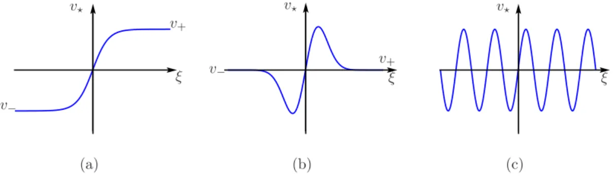
In Definition 2.1 we intentionally left the notion of a solution imprecise and we did also not specify the form of the (nonlinear) differential operator F. This will become clearer with the following examples. Generally, we assume a travelling wave to be continuously differentiable and bounded, i.e. the functionv⋆ is continuously differentiable and bounded. Figure 2.1 shows some wave profiles v⋆ of travelling waves, namely a front in (a), a pulse in (b) and a wavetrain in (c).
v⋆
ξ v+
v−
(a)
v⋆
ξ v+
v−
(b)
v⋆
ξ
(c)
Figure 2.1. Profile v⋆: front (a), pulse (b), and wavetrain (c).
Finding travelling waves in one space dimension can be reduced to searching for special solutions of ODEs. For that purpose assume (2.1) to have the more specific form
(2.4) ut=f(u, ∂xu, . . . , ∂xku), x∈R, t ≥0,
where f : R(k+1)m → Rm is a given nonlinearity. We insert the travelling wave ansatz
(2.5) u(x, t) =v(x−ct), x∈R, t≥0 into (2.4) and find
−cv′(x−ct) =f(v(x−ct), v′(x−ct), . . . , v(k)(x−ct)), x∈R, t≥0.
Since this should hold for all arguments we can substitute the wave variable ξ = x−ctand obtain the equation
0 = cv′(ξ) +f(v(ξ), v′(ξ), . . . , v(k)(ξ)), ξ ∈R,
which is a k-th order ODE on the real line. We usually suppress arguments and write this travelling wave ODEas
(TWODE) 0 =cv′+f(v, v′, . . . , v(k)), ξ∈R.
Note that the final step of reducing to an autonomous ODEs does not work if the functionf in (2.4) depends explicitly on xor t
ut=f(x, t, u, ∂xu, . . . , ∂xku), x∈R, t ≥0.
We will call (TWODE) the travelling wave ODE for the given PDE (2.4).
2.2. Examples from linear PDEs.
Example 2.2(The advection equation). Consider theadvection equation(orlinear transport equation)
(2.6) ut+aux = 0, x∈R, t ≥0
for some06=a∈R. The travelling wave ODE of (2.6) is 0 =cv′−av′, ξ∈R.
For nonconstant v we have v′ 6= 0 which implies c = a. Therefore, any function u⋆(x, t) = v⋆(x−at) with sufficiently smooth profile v⋆ (i.e. v⋆ ∈ C1(R,R)) is a travelling wave solution of (2.6) with speed c⋆ =a. In fact, the associated Cauchy problem of (2.6)
ut+aux= 0, x∈R, t≥0, u(x,0) =u0(x), x∈R, (2.7)
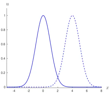
admits the solution u(x, t) = u0(x − at). That is all solutions of this simple equation are travelling waves (which, in a sense, is boring). For constant initial data, the solution is the same, but the speed is arbitrary. We consider this to be a degenerate situation since constants are steady states of the evolution equation (2.6) (i.e. ux = 0) while nonconstant profiles do not have this property. We sometimes call the latter ones true (or nontrivial) travelling waves. A travelling pulse solution of (2.6) is shown in Figure 2.2.
Example 2.3 (The heat equation). Consider the heat equation(or diffusion equa- tion)
(2.8) ut=auxx, x∈R, t ≥0,
for some0< a∈R. The travelling wave ODE of (2.8) is 0 =cv′+av′′, ξ ∈R, which has the two linearly independent solutions
(2.9) v1(ξ) = 1, v2(ξ) = e−caξ, ξ∈R.
Both are either constant or unbounded. We conclude that the heat equation has no true bounded travelling wave solutions. Later on, we will learn that this changes dramatically when we introduce nonlinearities into the heat equation.
Example 2.4 (The Klein Gordon equation). Consider the Klein Gordon equation (2.10) utt =a2uxx−µ2u, x∈R, t≥ 0
for some06=a, µ∈R. It is an easy exercise to show that the scaling
˜
u(y, s) =u(a µy, 1
µs)
-4 -2 0 2 4 6 8 0
0.2 0.4 0.6 0.8 1
x u
Figure 2.2. Travelling pulse solution u⋆(x, t) = v⋆(x−c⋆t) of the advection equation (2.6) with profile v⋆(ξ) = exp(−ξ22) and velocity c⋆ =a= 1 at time t= 0 (solid line) and t = 4 (dashed line).
transforms equation (2.10) into
(2.11) utt =uxx−u,
where the tilde was dropped and (y, s) was renamed as (x, t) for convenience.
Applying the travelling wave ansatz (2.5) to (2.11) leads to the travelling wave ODE of (2.11)
(2.12) 0 = (c2−1)v′′+v, ξ∈R,
which is now a second order ODE. Note that second order time derivative in (2.11) always imply a second order derivative in the associated traveling wave ODE (2.12).
The characteristic polynomial of (2.12)
p(λ) = (c2−1)λ2+ 1.
Solving (2.12) is equivalent to finding zeros of p, i.e. λ with p(λ) = 0, which are
λ=
(±√11−c2, |c| 6= 1 no zeros, |c|= 1 =
±√ 1
|c2−1|, |c|<1 no zeros, |c|= 1
±i√ 1
|c2−1|, |c|>1 .
-10 -5 0 5 10 -4
-3 -2 -1 0 1 2 3 4
x u
Figure 2.3. Travelling wavetrain solution u⋆(x, t) = v⋆(x − c⋆t) of the Klein Gordon equation (2.10) for k = 1, α1 = 2, α2 = 3, c= ω(k)k =√
2 at timet= 0 (solid line) and t= 1 (dashed line).
If|c| = 1 the equation p(λ) = 0, hence also the equation (2.12), has no solutions.
If|c| 6= 1 the fundamental solutions of the linear equation (2.12) are v1(ξ) =
cosh(kξ), |c|<1
cos(kξ), |c|>1 , v2(ξ) =
sinh(kξ), |c|<1 sin(kξ), |c|>1 , where the quantity k denotes the angular wave number defined by
(2.13) k = 1
p|c2−1|.
In case |c| < 1 there is no bounded solution whereas in case |c| > 1 we have the linear family of bounded solutions
(2.14) v(ξ) = α1cos(kξ) +α2sin(kξ), α1, α2 ∈R.
Defining theangular frequencyω(k) :=ck, we obtain the family of travelling waves (2.15) u(x, t) =α1cos(kx−ω(k)t) +α2sin(kx−ω(k)t), x, t∈R, α1, α2 ∈R. The definition of ω(k) and equation (2.13) imply the relation
(2.16) ω(k)2 =k2+ 1,
which is called thedispersion relation. This relation shows how the speed cof the wave is related to its frequency ω(k). In fact, multiplying (2.13) by the velocity c
shows that (2.16) is equivalent to
ω(k) = c p|c2−1|.
For completeness, recall the following relations from the theory of wave equations k = ω
c = 2π
λ = 2πν c ,
where k is the angular wave number (or: magnitude of the wave vector), ν the frequency of the wave, λ the wavelength, ω = 2πν the angular frequency of the wave and cthe phase velocity.
Note that the travelling waves (2.15) are neither fronts nor pulses but have an oscillatory character. For this reason they are called wave trains. Contrary to Example2.2, the wave trains (2.15) do not have a fixed speed but can travel at all speeds c >1 and c <−1.
Example 2.5 (Symmetric hyperbolic systems). A direct generalization of the ad- vection equation (2.6) is the first order system
(2.17) ut+Aux = 0, u:R×[0,∞)7→Rm, A∈Rm,m.
The travelling wave ODE reads (A−cIm)v′ = 0. Every real eigenvalue with real eigenvector
(2.18) Aw=λw, λ ∈R, w ∈Rm
leads to a solution
(2.19) v(ξ) =α(ξ)w,
where α : R 7→ R is any bounded sufficiently smooth function. This corresponds to the travelling wave solution
(2.20) u(x, t) =α(x−λt)w.
If A is real diagonalizable, then it has only real eigenvalues λj with linearly in- dependent eigenvectors wj, j = 1, . . . , m. Correspondingly, equation (2.17) has solutions which are superpositions of waves travelling with speed λj in direction wj
(2.21) u(x, t) =
Xm j=1
αj(x−λjt)wj,
where the αj are smooth bounded scalar functions. Given an initial condition as in (2.7) with a vector valued function u0, the solution of the Cauchy problem (2.17),(2.7) is given by (2.21), where the functions αj are determined from the decomposition of initial data
u0(x) = Xm
j=1
αj(x)wj, x∈R.
We conclude that all solutions of the first order system (2.17) are linear super- positions of travelling waves with different speeds. The system (2.17) is called symmetric because we can transform (2.17) via
u(x, t) =W v(x, t), W = w1 w2 · · · wm
∈Rm,m into the diagonal system
vt+ diag(λj, j = 1, . . . , m)vx = 0,
which consists of m copies of the advection equation (2.6) with different propaga- tion speeds.
2.3. Travelling waves in nonlinear parabolic PDEs. We are looking for trav- elling waves in a nonlinear system of equations
(2.22) ut=Auxx+f(u), x∈R, t≥0,
where f ∈ C1(Rm,Rm) and A ∈ Rm,m is invertible. By (TWODE) the travelling wave ODE is
(2.23) 0 = Av′′+cv′+f(v).
We look for solutions v ∈C2(R,Rm)of this system such that the limits v±= lim
ξ→±∞v(ξ), v±′ = lim
ξ→±∞v′(ξ) exist. As the next Lemma shows, this necessarily implies
(2.24) f(v±) = 0, lim
ξ→±∞v′(ξ) = 0.
Lemma 2.6. With the setting w= v
v′
equation (2.23) is equivalent to the first order system
(2.25) w′ =
w2
−cA−1w2−A−1f(w1)
=:G(w).
Any solution of (2.23) on [0,∞) for which the limits
ξlim→∞v(ξ) =:v+, lim
ξ→∞v′(ξ) =:v+′ exist, satisfy
(2.26) f(v+) = 0, v′+= 0.
The same statement holds if the limitsξ → −∞ exist.
Proof. The transformation to a first order system is standard. Fromw(ξ)→w+ :=
v+
v+′
as ξ→ ∞ we obtain for allx≥0
|G(w+)|=
Z x+1 x
G(w+)−G(w(ξ)) +w′(ξ)dξ
≤ Z x+1
x |G(w+)−G(w(ξ))|dξ+|w(x+ 1)−w(x)|
≤sup
ξ≥x|G(w+)−G(w(ξ))|+|w(x+ 1)−w+|+|w+−w(x)|.
By our assumption and the continuity of G the right hand sides converge to 0 as x→ ∞. Hence, w+ satisfies G(w+) = 0 from which (2.26) follows.
Remark 2.7. If all eigenvalues of A have positive real part (i.e. equation (2.22) is parabolic) then one can omit the assumption that the derivative v′(ξ) converges as ξ→ ±∞. This will be proved in Lemma 2.23 in Section 2.6.
Another simple observation is the following reflection symmetry.
Lemma 2.8. If v⋆, c⋆ is a travelling wave of the system (2.22) then so is (2.27) v⋆(ξ) = v⋆(−ξ), c⋆ =−c⋆.
In the following we restrict to scalar equation withA= 1 (2.28) ut=uxx+f(u), x∈R, t≥0, with travelling wave ODE
(2.29) 0 =v′′+cv′+f(v).
According to Lemma2.6 the potential limits of travelling waves must be zeroes of f. In the following we are particularly interested in the case where f has three zeroes
(2.30) b1 < b2 < b3 and f(v)
>0, v < b1, b2 < v < b3
<0, b1 < v < b2, b3 < v . Our model example is the following Nagumo equation
Example 2.9 (Nagumo equation). Consider the scalar parabolic equation ut=uxx+u(1−u)(u−b), x∈R, t ≥0,
(2.31)
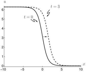
where 0< b < 1, [21], [22]. It is well known that (2.31) has an explicit travelling front solution u⋆(x, t) =v⋆(x−c⋆t)(called the Huxley wave) given by
v⋆(ξ) = 1 1 +exp
−√ξ2, c⋆ =√ 2
b− 1
2 (2.32) ,
with asymptotic statesv−= 0 and v+ = 1. Note that c⋆ <0 if b < 12 and c⋆ >0 if b > 12.
Demo: Phase plane analysis of (2.25),(2.29)
In Mathematical Biology this equation is motivated by population models which have three equilibria as in (2.30) in the spatially independent case. An example of this is the spruce budworm model described in [22, Ch.1.2, Ch.11.5]
ut=ru
1− u q
− u2 1 +u2.
If one adds spatial spread of populations via diffusion to such a law then a parabolic equation of the type (2.28) arises with the nonlinearity satisfying (2.30).
The following exercise shows that systems with cubic nonlinearities which have 3 consecutive zeros and behave like−u3 (rather than u3) can always be transformed into the Nagumo equation (2.31).
Exercise 2.10. Show that the general equation
(2.33) ut=Duxx+B(u−b1)(b2 −u)(u−b3), x∈R, t≥0
where D, B > 0 can be reduced to the Nagumo equation (2.31) via linear trans- formations u = β1u˜ +β2 and scalings of time and space u(x, t) = ˜u(α1x, α2t).
Determine the profile and speed of a travelling wave for (2.33).
Solution: The linear transformationu= b1+ ˜u(b3−b1) shifts the zeroesb1, b2, b3 to 0, b =
b2−b1
b3−b1,1 and gives the equation ut=(b3−b1)˜ut
=D(b3−b1)˜uxx+B(b3−b1)˜u(b2−b1−(b3−b1)˜u)(b3−b1)(˜u−1),
˜
ut=Du˜xx+B(b3−b1)2u(b˜ −u)(˜˜ u−1).
Now perform a scalingu(x, t) = ˜˜ u(α˜ 1x, α2t)and obtain
˜
ut=α2u˜˜t=α21Du˜˜xx+B(b3−b1)2u(b˜˜ −u)(˜˜˜ u˜−1).
This is equivalent to (2.31) if we set
α2=B(b3−b1)2, α1= rα2
D = (b3−b1) rB
D.
Suppose˜˜u(x, t) =v⋆(x−c⋆t)is travelling wave of (2.31) then we have the following solution of (2.33)
u(x, t) =b1+ (b3−b1)v⋆(α1x−c⋆α2t).
This is a travelling wave with speed
(2.34) c˜=c⋆
α2
α1
=c⋆
√DB(b3−b1)
and profile
(2.35) v(ξ) =˜ b1+ (b3−b1)v⋆(α1ξ), α1= (b3−b1) rB
D.
With the values ofbandc⋆ from (2.32) we obtain the final expression for the speed of the wave that belongs to (2.33)
˜ c=√
2
b2−b1
b3−b1−1 2
(b3−b1)√ DB=
rDB
2 (−b1+ 2b2−b3).
(2.36)
Although it is easy to verify the formula (2.32) for the travelling wave of the Nagumo equation (2.31), we discuss a more general approach that allows to arrive at such an explicit expression. The travelling wave ODE for (2.31) is
(2.37) 0 =v′′+cv′ +v(v−b)(1−v).
Note that the standard energy method for ODEs works only in case c = 0 (cf.
Section 2.4). In order to find a solution which connects v− = 0 tov+ = 1 we try a solution of the first order equation
(2.38) v′ =αv(1−v) =: g(v),
where the parameter α > 0 is still to be determined. By separation of variables, the solution of (2.38) withv(0) = 12 is found to be
(2.39) vα(ξ) = 1
1 +exp(−αξ), ξ∈R.
We insert (2.38) into (2.37):
vα′′+cvα+vα(b−vα)(vα−1) =g′(vα)vα′ +cv′α− 1
α(b−vα)vα′
=vα′
−2αvα+α+c− b α+ 1
αvα
. This term vanishes provided we set
α= 1
√2, c⋆ = b
α −α =√
2(b− 1 2), which together with (2.39) leads to formula (2.32).
The following proposition summarizes the general methodology.
Proposition 2.11. Letg ∈C1(Rm,Rm) satisfy for some c∈R (2.40) (Dg(v) +cIm)g(v) +f(v) = 0, ∀v ∈Rm.
Then any solution v ∈C1(J,Rm)of v′ =g(v) on some intervalJ ⊆Rsatisfies the travelling wave ODE (2.29) on J.
Proof. It is sufficient to note thatv′ =g(v)onJ impliesv′′ =Dg(v)v′ =Dg(v)g(v)
onJ by the chain rule.
Remark 2.12. For the Nagumo equation (2.31) we used this proposition with the settings f(v) = v(b−v)(v−1), g(v) =αv(1−v) where α and c were determined such that (2.40)holds. If, in the scalar case, g is taken to be a polynomial of degree ℓ, then f should be a polynomial of degree 2ℓ−1. Moreover, relation (2.40) shows thatg is a smooth factor off, i.e. the zeroes of g are also zeroes of f and if f has even more real zeroes, then they must be incorporated into the first factorg′(v) +c.
Exercise 2.13. Consider the quintic Nagumo equation
(2.41) ut=uxx −
Y5 i=1
(u−bi),
where b1 < b2 < b3 < b4 < b5 . Determine a relation among b1, . . . , b5 that allows to compute a travelling wave connection ofb1 tob3 or of b3 tob5 from a first order ODE.
2.4. Phase plane analysis of travelling wave ODEs. As shown in Lemma 2.6, the profile of a travelling wave appears as an orbit connecting two steady states of an autonomous ODE.
Definition 2.14. Let w∈C1(R,Rm) be a solution of the dynamical system (2.42) w′ =G(w), where G∈C1(Rm,Rm),
such that the limits
(2.43) lim
ξ→±∞w(ξ) =w±
exist. Then Q(w) = {w(ξ) : ξ ∈R} is called an orbit connecting the steady state w− to the steady state w+. The connecting orbit is called heteroclinic if w−6=w+, and homoclinic if w− =w+.
Therefore, a travelling wave of equation (2.22) with speed c⋆ and profile v⋆ con- necting v− to v+, corresponds to an orbit Q(w⋆), w⋆ =
v⋆
v⋆′
of the dynamical system (2.25) with parameter c= c⋆ connecting the steady state w− =
v− 0
to w+ =
v+
0
. We stress the fact that not only the orbit w⋆ but also the speedc⋆ is unknown. Therefore, we have to drive the system (2.25) by varyingcuntil an orbit connecting two steady states occurs. Proving that such a connection occurs can be quite hard, and we refer to Section3 for some situations where this is possible.
Before treating further examples we add another observation that applies to trav- elling waves of (2.22) for which the nonlinearityf is a gradient, i.e.
(2.44) f(v) = ∇F(v), v ∈Rm for some F ∈C2(Rm,R).
Proposition 2.15. Let A ∈ Rm,m be symmetric and let f ∈ C1(Rm,Rm) be the gradient of someF ∈C2(Rm,R). Further, letv∗ ∈C2(R,Rm)be a travelling wave of (2.22) with speed c∗ 6= 0, connecting v− to v+. Then, v⋆′ ∈ L2(R,Rm) and the following formula holds
(2.45) c⋆
Z ∞
−∞|v⋆′(ξ)|2dξ =F(v−)−F(v+).
Proof. Multiply the travelling wave ODE (2.23) byv⋆′T and integrate over [−R, R]
(2.46)
Z R
−R
v⋆′(ξ)TAv⋆′′(ξ)dξ+c⋆
Z R
−R|v⋆′(ξ)|2dξ=− Z R
−R
v⋆′(ξ)T∇F(v⋆(ξ))dξ.
Integration by parts and the symmetry ofA show for the first integral Z R
−R
v′⋆(ξ)TAv′′⋆(ξ)dξ = 1
2 (v⋆′)2(R)−(v′⋆)2(−R) ,
which converges to zero as R → ∞. The right hand side in (2.46) is a complete integral
Z R
−R
v⋆′T(ξ)T∇F(v⋆(ξ))dξ = Z R
−R
d
dξ(F ◦v⋆)(ξ)dξ =F(v⋆(R))−F(v⋆(−R)), which converges to F(v+)−F(v−). Therefore, we can take the limit R → ∞ in (2.46) and obtainv′∗ ∈L2(R,Rm) as well as formula (2.45).
Formula (2.45) shows that the speed c⋆ of the wave is positive if F(v−) > F(v+) and negative if F(v−)< F(v+), i.e. the wave runs from the larger critical value of the potentialF to the smaller critical value. This imposes restrictions on the type of transitions that a wave can take. Note that c⋆ = 0 still follows from our proof in caseF(v−) =F(v+), but we cannot conclude v⋆′ ∈L2(R,Rm)anymore.
Proposition2.15 always applies to the scalar case which has the potential
(2.47) F(ξ) =
Z ξ 0
f(x)dx.
In the scalar case (2.28), the system (2.25) becomes two-dimensional
(2.48) w′ =
w1′ w2′
=
w2
−f(w1)−cw2
=:G(w), and much insight can be gained by so-called phase plane analysis.
Lemma 2.16. Let v0 ∈ R be a zero of f. Then the steady state w0 = v0
0
of (2.48) is a
saddle if f′(v0)<0,
sink if f′(v0)>0andc >0, source if f′(v0)>0andc <0.
More precisely, the eigenvalues of the linearization
(2.49) DG(w0) =
0 1
−f′(v0) −c
are
(2.50) λ±= 1
2
−c±p
c2−4f′(v0) .
In case of a saddle the eigenvalues satisfy λ− <0 < λ+ and suitable eigenvectors are
(2.51) y−=
1 λ−
, y+ = 1
λ+
.
Proof. The proof follows by straightforward computation of the eigenvalues and eigenvectors of the Jacobian (2.49). Note that in the borderline casesf′(v0) = 0and f′(v0)>0, c = 0the linearization is not enough to determine the type of the steady state since some eigenvalues lie on the imaginary axis (in casef′(v0) = 0, c <0one can at least conclude that w0 is unstable). Also note that the eigenvalues become complex if
(2.52) c2 <4f′(v0),
i.e. the solutions are spiraling in if c >0and spiraling out if c <0.
Remark 2.17. The qualitative phase diagram near steady states is preserved from the linear to the nonlinear case provided there are no eigenvalues on the imaginary axis. This is made precise by the famous Hartman-Grobman theorem, see for exam- ple [4, Theorem 19.9]. Given a dynamical system v′ =f(v) with f ∈C1(Rm,Rm) and t-flow denoted by ϕt. Let v0 ∈ Rm be a steady state such that Df(v0) has no eigenvalues on the imaginary axis and let Φt(v) = exp(tDf(v0))v be the lin- earized flow. Then there exist neighborhoods U ⊆ Rm of 0, V ⊆ Rm of v0 and a homeomorphism h:U →V such that
(2.53) ϕt◦h(v) = h◦Φt(v)
holds for all (t, v) with Φs(v) ∈ U for all min(t,0)≤ s ≤max(t,0). The relation (2.53) is also called local flow equivalence.
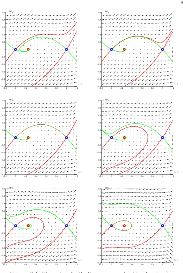
Demo: The following Figure shows the (numerical)
c1 =−0.4<c2 =−0.36< c3 =−0.35355339≈c⋆
<c4 =−0.3< c5 =−0.2< c6 = 0.
Since f′(0) <0 and f′(1) < 0 both steady states w− = (0,0) and w+ = (1,0) are saddles. The eigenvectors from (2.51) are locally tangent to the so called stable and unstable manifolds
(2.54) Ws(w±) ={w:ϕξ(w)→w± asξ → ∞}
Wu(w±) ={w:ϕξ(w)→w± asξ → −∞},
where ϕξ denotes the ξ-flow of the system (2.48). We used the variable ξ instead of t since ξ is the wave variable by derivation. Sometimes this approach is called spatial dynamics. As we will see in Section 3, the stability of travelling waves for the time-dependent PDE (2.22) has nothing to do with the stability properties of the asymptotic steady states when considered as equilibria of the travelling wave ODE.
In the current example the one-dimensional unstable manifold ofw− and the one- dimensional stable manifold of w+ intersect at a specific value of c. Then they must coincide because of uniqueness of solutions to initial value problems to form a heteroclinic orbit.
We also observe that there are orbits connecting the sourcewb = (b,0)to the saddle w− = (0,0). These are also travelling waves for the original PDE, but as we will see, the corresponding solutions of the PDE (2.22) do not enjoy the same favorable stability properties as the saddle-to-saddle connection. Moreover, they occur over a whole interval ofc-values since wb has a two dimensional unstable manifold and w− has a one-dimensional stable manifold.
The classical example for such waves is the Fisher equation ([22, Ch.11.4],[10, Ch.4.4] for which, unfortunately, there is no general explicit formula for the trav- elling wave solution (except for the nontypical speedc= √56, see [24]).
Example 2.18(The Fisher equation). On assumes logistic growth of a population and diffusion
(2.55) ut=uxx+u(1−u), x∈R, t≥0, with the travelling wave ODE given by
(2.56) 0 =v′′+cv′+v(1−v).
The steady states are v0 = 0 and v1 = 1 with f′(v0) = 1, f′(v1) = 1. From Lemma 2.16 we immediately infer for the system (2.48) that
(2.57)
v+ :=
1 0
is a saddle,
v− :=
0 0
is
an unstable node, c <−2, a spiral source, −2< c <0,
a spiral sink, 0< c <2, a stable node, 2< c.
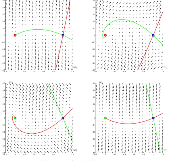
We are looking for a connection from v− to the saddle v+ and we restrict toc <0 since the case c > 0 follows by reflection (cf. Lemma 2.8). Moreover, since the equation models populations, we are only interested in solutions that haveu(ξ)≥0 for all ξ ∈ R. The phase diagram reveals that the stable manifold of the saddle (approachingv+ through negative values ofv′) originates from the unstable node/
spiral source at v− . The positivity condition on v excludes the case of a spiral source for −2 < c < 0. Therefore, we have a whole family of connecting orbits v(·, c)for parameter valuesc≤ −2(by a limit argument one can show that the orbit fromv− tov+ is also nonegative for c =−2). In view of the phase portraits near an unstable node it is also reasonable to expect that the connecting orbit leavesv− in the direction of the eigenvector that belongs to the ’slowest eigenvalue’. In view of (2.50) and (2.51) this direction is y− =
λ− 1
where λ− = 12 −c−√
c2 −4 . In the critical casec⋆ =−2we have λ− =λ+ = 1.
Since we find a whole family of positive travelling waves (c≤ −2), it is a natural question to ask, which one of these appears in the longtime dynamics of the PDE (2.54) when initial datau(·,0) =u0(·)far from the true waves are given. This is a delicate matter which depends sensitively on the behavior of the data u0 at ±∞. In a sense the critical wave at c = −2 is the ’most stable’ one concerning these conditions (see the discussion in [22, Ch.11.2]).
2.5. Examples of nonlinear wave equations. As in Section 2.3 for the para- bolic case, we now consider some nonlinear versions of the linear wave equations from Section2.2.
Example 2.19. Consider the nonlinear wave equation (2.58) utt =uxx−sinu, x, t∈R Exercise 2.20. Show that the general equation
Autt =Kuxx−T sin(u), A, K, T >0 can be cast into the form (2.58) by suitable transformations.
The travelling wave ODE for (2.58) reads
(2.59) (c2−1)v′′=−sin(v).
In the following we assume |c| 6= 1. The only steady states of the corresponding first order system are wn = (vn,0) = (nπ,0), n ∈ Z. As in Lemma 2.16 saddles occur for even values ofn, while wn are centers for odd values of n (this, however, does not follow from Lemma2.16). We look for an explicit solution that connects w2 to w0.
An explicit solution may be found by the energy method: multiply by v′ and integrate,
(c2−1)v′′v′ =(c2−1)[1
2(v′)2]′ = [cos(v)]′ =−sin(v)v′, const =c2−1
2 v′(ξ)2−cos(v(ξ)) ∀ξ∈R.
Since we want a solution with v(ξ) → 0, v′(ξ) → 0 as ξ → ∞ (resp.v(ξ) → 2π, v′(ξ)→0 asξ → −∞) we find the constant const =−1. Thus we have to solve
(2.60) (v′)2 = 2
1−c2(1−cos(v)), ξ∈R.
Since the left-hand side is nonnegative and 1−cos(v) ≥ 0 the only case left is
|c|<1. Then a solution to (2.60) is found by separation of variables as (2.61) v⋆(ξ) = 4arctan (exp(− ξ
√1−c2)), ξ∈R.
The corresponding travelling waves u(x, t) =v⋆(x−ct) exist for all |c|<1.
Demo: c= 12
As shown above the system (2.59) has a conserved quantity E(v, v′) = c2−21(v′)2− cos(v). Hence the phase plane consists of the level curves ofE, apart from homo- clinic orbits there are also continua of periodic orbits which lead to wave trains.
The next example contains third order spatial derivatives. It is derived by simpli- fying equations for water waves and to approximately describe the propagation of solitary waves, compare [31, Ch.13.11].
Example 2.21 (The Korteweg-de Vries (KdV) equation). The equation is the following
(2.62) ut=−uux−uxxx, x∈R with travelling wave ODE
(2.63) 0 = cv′− 1
2(v2)′−v′′′. Integrating once leads to
(2.64) v′′=cv−1
2v2 =v(c− 1
2v) =:f(v).
We took the integration constant to be zero since we look for solutions satisfying v(ξ)→0and v′′(ξ)→0 as ξ→ ±∞.
Equation (2.64) can be handled completely by the energy method since it has the conserved quantity
(2.65) E(v) = 1
2(v′)2+P(v), P(v) =− Z v
0
f(s)ds=−c
2v2+ 1 6v3.
Here P is the potential satisfying P′ = −f, and (2.64) may be considered as the Newtonian dynamics of a particle of mass 1 moving in the potential P. The first order system has a homoclinic orbit connecting(0,0)to itself which belongs to the energy level E(v) = 0 and, for c >0, is explicitly given by
(2.66) v(ξ) = 3csech2(
√c
2 ξ), ξ∈R.
Thus the KdV equation has a whole family of solitary waves given by u(x, t) = 3csech2(
√c
2 (x−ct)), c >0.
Demo: travelling wave and phase plane diagram for KdV 2.6. Travelling waves in parabolic systems.
Example 2.22(FitzHugh-Nagumo system). Consider the2-dimensional FitzHugh- Nagumo system
ut=
1 0 0 ρ
uxx+
u1− 13u31−u2
ε(u1+a−bu2)
, x∈R, t≥0, (2.67)
with u=u(x, t)∈R2 and positive ρ, a, b, ε∈ R, [11]. For the parameters ρ= 0.1, a = 0.7, ε = 0.08 it is well-known that (2.67) has travelling pulse solutions for b= 0.8 and travelling front solutions forb = 3. Unfortunately, in both cases there are no explicit representations neither for the wave profilew⋆ nor for their velocities c⋆. However, we know some approximations of the velocities in both cases. The pulse travels at velocity c⋆ =−0.7892 and the front at velocity c⋆ =−0.8557.
In fact, the value ofbdetermines the number of steady states of (2.67) (for bsmall we have only one steady state but forb large we have three).
The next Lemma improves Lemma 2.6 by showing that the convergence of a trav- elling wave to its limits implies the convergence of derivatives. In fact, ifv satisfies the travelling wave ODE (2.23) and v± = limξ→±∞v(ξ) exist, then the following Lemma applies toh(ξ) =−f(v(ξ)), ξ∈R and shows
f(v±) = 0, lim
ξ→±∞v′(ξ) = 0.
Lemma 2.23. Let A ∈ Rm,m have only eigenvalues with positive real part and suppose v ∈C2(R,Rm) and c∈R solve the second order ODE
(2.68) Av′′+cv′ =h ∈C(R,Rm),
such that both limits limξ→±∞h(ξ) and limξ→±∞v(ξ) exist. Then the following equalities hold
(2.69) lim
ξ→±∞h(ξ) = 0 = lim
ξ→±∞v′(ξ).
Proof. It is sufficient to prove the result for the positive axisR+ = [0,∞), then the result for the negative axis follows by reflection since we have made no assumption on the sign ofc. First multiply (2.68) by A−1 to obtain
(2.70) v′′+cA−1v′ =A−1h=:r,
ξlim→∞r(ξ) =A−1 lim
ξ→∞h(ξ) =:r+. All solutions of (2.70) can be written as follows
(2.71) v(ξ) =V1(ξ)α1+V2(ξ)α2+v3(ξ), ξ ∈R, α1, α2 ∈Rm, where
V1 V2
V1′ V2′
∈R2m,2m forms a fundamental system of the first order equation obtained from (2.70) and v3 is a special solution of the inhomogenous equation.
We will construct v3 in the following form
(2.72) v3(ξ) =
Z ∞
0
G(ξ, η)r(η)dη, ξ∈R
with a suitable Green’s matrix G. We will use the boundedness of v to show that v3(ξ)is the dominant part in (2.71) and that |v3(ξ)| → ∞ asξ→ ∞ if r+ 6= 0.
c >0: Take V1(ξ) =Im,V2(ξ) = Aexp(−cA−1ξ)and (2.73) G(ξ, η) =
1
cA(Im−exp(−cA−1(ξ−η))), 0≤η≤ξ,
0, ξ < η.
One easily verifies thatV1, V2 generate fundamental solutions and that v3
satisfies the inhomogeneous equation (2.70) as well asv3(0) =v3′(0) = 0.
Let us note that all eigenvalues of A−1 have positive real part, hence there exists ρ1 >0such that Re(µ)<−ρ1 for all eigenvalues µof −A−1. By a well-known result (see Numerical Analysis of Dynamical Systems, for example) we then have a constant C >0 such that
(2.74) |exp(−τ A−1)| ≤Cexp(−ρ1τ), τ ≥0.
Since V1, V2 and v itself are bounded, equation (2.71) implies that v3 is bounded. We now assume r+6= 0 and show that |v3(ξ)| ≥Cξ for ξ large which is a contradiction. Given ε >0, take ξε so large that
|r(ξ)−r+| ≤ε for all ξ ≥ξε. Then we estimate with (2.74)
|v3(ξ)| ≥
Z ξ ξε
G(ξ, η)dηr+
−
Z ξε
0
G(ξ, η)r(η)dη
−
Z ξ ξε
G(ξ, η)(r(η)−r+)dη
≥
A c
ηIm−A
cexp(−cA−1(ξ−η)) ξ
ξε
r+
−ε Z ξ
ξε
|G(ξ, η)|dη− Z ξε
0 |G(ξ, η)|dηkrk∞
≥ξ−ξε
c |Ar+| − 2C|A|2|r+|
c2 −ε(ξ−ξε)2C|A|
c − 2|A|Ckrk∞ξε
c .
Since |Ar+|>0, the third term can be absorbed into the first one by tak- ing ε sufficiently small, which then dominates the second and the fourth one by taking ξ−ξε sufficiently large. This shows that v3 is unbounded, a contradiction.
Finally, we obtain from (2.71)
v′(ξ) =V2′(ξ)α2+v3′(ξ), ξ∈R.
The first term decays exponentially due to (2.74). The second term is v3′(ξ) =
Z ξ 0
exp(−cA−1(ξ−η))r(η)dη.
With (2.74) we estimate v3′ as follows
|v3′(ξ)| ≤ Z ξ/2
0 |G(ξ, η)|dηkrk∞+ Z ξ
ξ/2|G(ξ, η)||r(η)|dη
≤C
(Z ξ/2 0
exp(−cρ1(ξ−η))dηkrk∞+ Z ξ
ξ/2
exp(−cρ1(ξ−η))dη sup
η≥ξ/2|r(η)| )
≤ C cρ1
exp(−cρ1ξ
2 )−exp(−cρ1ξ)
krk∞
+
1−exp(−cρ1ξ 2 )
sup
η≥ξ/2|r(η)| )
.
Since r+ = 0 and c, ρ1 > 0 all terms on the right-hand side converge to zero as ξ→ ∞.
c= 0: The fundamental matrices are V1(ξ) = Im, V2(ξ) = ξIm and Green’s matrix is given by
(2.75) G(ξ, η) =
(ξ−η)Im, η ≤ξ, 0, η > ξ.
Assume r+ 6= 0and for a given ε >0 takeξε such that|r(η)−r+| ≤εfor all η≥ξǫ. Then we estimate
|v3(ξ)| ≥|
Z ξ ξε
(ξ−η)dη r+|
−|
Z ξ ξε
(ξ−η)(r+−r(η))dη| − | Z ξε
0
(ξ−η)r(η)dη|
≥1
2(|r+| −ε)(ξ−ξε)2− krk∞ξε(ξ−1 2ξε).
By taking ε sufficiently small and letting ξ → ∞, we find that v3 grows quadratically if r+ 6= 0. This is stronger than α1+V2(ξ)α2 which grows at most linearly, and contradicts the boundedness of v3.
Equation (2.68) has the simple form v′′ =r and we have to show that limξ→∞r(ξ) = 0and the existence oflimξ→∞v(ξ)implylimξ→∞v′(ξ) = 0.
Without loss of generality we can assume m = 1. Then the mean value theorem implies that
v(n+ 1)−v(n) = v′(θn) for some θn ∈(n, n+ 1).
Since v(n) and v(n + 1) have the same limit, we infer v′(θn) → 0 as n → ∞. Therefore, forn ≤ξ ≤n+ 1
|v′(ξ)| ≤|v′(ξ)−v′(θn)|+|v′(θn)|
≤ sup
η∈[n,n+1]|v′′(η)||ξ−θn|+|v′(θn)|
≤ sup
η∈[n,n+1]|v′′(η)|+|v′(θn)| →0 as n→ ∞.
c <0: As in case c > 0 we use the fundamental matrices V1(ξ) = Im and V2(ξ) = Aexp(−cA−1ξ), however the Green’s matrix is no longer a trian- gular kernel
(2.76) G(ξ, η) = A c
Im−exp(cA−1η), η ≤ξ,
exp(cA−1(η−ξ))(Im−exp(cA−1ξ)), η > ξ.
Note that (2.74) and c <0imply for some constant C1 >0the estimate (2.77) |G(ξ, η)| ≤C1
1, η ≤ξ, exp(−|c|ρ1(η−ξ)), η > ξ.
Therefore, the integral in (2.72) exists and yields the estimate
| Z ∞
0
G(ξ, η)r(η)dη| ≤ Z ∞
0 |G(ξ, η)|dηkrk∞≤C1(ξ+ 1
ρ1|c|)krk∞.
It is then straightforward to verify that (2.72) yields a solution of (2.68) which grows at most linearly with ξ. Therefore, the dominant term in (2.71) is
|V2(ξ)α2|=|exp(−cA−1ξ)Aα2| ≥exp(|c|ρ1ξ)|Aα2|.
Since v is bounded we conclude that α2 = 0. Let us assume r+ 6= 0 and estimate v3 from below with ξε chosen as in the previous cases:
|v3(ξ)| ≥|
Z ∞
ξε
G(ξ, η)dη r+| − | Z ξε
0
G(ξ, η)r(η)dη|
−|
Z ∞
ξε
G(ξ, η)(r+−r(η))dη|. For the first integral we find
Z ∞
ξε
G(ξ, η)dη=A c
ηIm− A
cexp(cA−1η) ξ
ξε
−A
c(Im−exp(cA−1ξ)) A
cexp(cA−1(η−ξ)) ∞
ξ
=A c
(ξ−ξε)Im+A
c(Im−exp(cA−1ξε))
, so that for some constants C1, C2 >0
(2.78) |
Z ∞
ξε
G(ξ, η)r+dη| ≥C1|ξ−ξε||Ar+| −C2.
For the third term we obtain from (2.77)
| Z ∞
ξε
G(ξ, η)(r+−r(η))dη≤ε Z
ξε
|G(ξ, η)|dη
≤ε(C1(ξ−ξε) +c2).
This term can be absorbed into (2.78) by taking ε sufficiently small. Fi- nally, equation (2.77) also leads to an estimate of the second term
| Z ξε
0
G(ξ, η)r(η)dη| ≤C1ξεkrk∞.
Summing up, if r+ 6= 0 we get a linearly growing lower bound for v3(ξ) which contradicts the boundedness of v.
Finally we have to show v′(ξ)→0 as ξ → ∞. For this note that from (2.76) we have
v3′(ξ) =− Z ∞
ξ
exp(cA−1(η−ξ))r(η)dη.
This yields the estimate
|v3′(ξ)| ≤sup
η≥ξ|r(η)|
Z ∞
ξ
exp(cA−1(η−ξ))dη
≤sup
η≥ξ|r(η)| Z ∞
ξ
exp(−ρ1|c|)dη= 1 ρ1|c|sup
η≥ξ|r(η)|, which shows v′(ξ) =v′3(ξ)→0as ξ → ∞and finishes the proof.
Remark 2.24. We notice that the convergence of v(ξ) as ξ → ±∞ was only used to derive v′(ξ)→0 in case c= 0. All other conclusions work under the hypothesis thatv is bounded.
2.7. Waves in complex-valued systems in one space dimension. Quite a few models in Physics lead to PDEs for complex-valued functions
(2.79) u:R×[0,∞)→C, (x, t)→u(x, t).
We just mention the well-known Schrödinger equation from quantum mechanics.
Thereu is a wave function with complex amplitude, the absolute value |u(x, t)|of which may be interpreted as the probability of finding the ’particle’ at position x at timet.
In this subsection we consider equations of the type
(2.80) ut=auxx+g(x,|u|)u, x∈R, t ∈R,
where a ∈ C and g : R2 → C is a smooth function. In case Re(a) > 0 the equation is of parabolic type while in casea =iit is of wave type (the Schrödinger
equation). This can be seen from the real-valued version of (2.80), which reads (witha =a1 +ia2,u=u1+iu2,g =g1+ig2):
(2.81)
u1
u2
′
=
a1 −a2
a2 a1
u1
u2
xx
+
g1 −g2
g2 g1
(x,|u|) u1
u2
. We consider some characteristic examples:
Example 2.25 (Linear Schrödinger equation (LSE)).
(2.82) a=i, g(x,|u|) =−iV(x), x∈R, V :R→Rpotential.
Note that in Physics one usually writes i~Ψt =−~2
2µ∆Ψ +V(x)Ψ
where ~ is Planck’s reduced constant and Ψ is the wave function. Dividing by i~
and scaling the space variable allows to reduce this to (2.80),(2.82). We prefer to keep the pure time derivative ut on the left-hand side in order not to change our general evolution equation (2.1).
Example 2.26 (Nonlinear Schrödinger equation (NLS)).
(2.83) a=i, g(x,|u|) =β|u|p, β =ib, b∈R, p≥2.
Forp= 2 we have the cubic nonlinear Schrödinger equation (CNLS).
Example 2.27 (The Gross-Pitaevskii equation (GPE)). This is a mixture of LSE and the cubic NLS and supposed to describe so-called Bose-Einstein condensates:
(2.84) a= 1
2i, g(x,|u|) =−iV(x) +β|u|2, β=ib, b∈R.
Example 2.28 (Complex Ginzburg-Landau equation). This equation occurs in applications to superconductivity, in nonlinear optics, and in laser physics:
(2.85) rm Im(a)6= 0,Re(a)>0, g(x,|u|) =µ+β|u|2+γ|u|4,
where typically µ ∈ R but β, γ ∈ C. In the case given here, the nonlinearity has quintic terms, therefore it is called the quintic complex Ginzburg-Landau equation (QCGL).
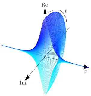
Rather than travelling waves we look for a standing oscillating pulse (sometimes called an oscillon)
(2.86) u(x, t) =exp(−iθt)v(x), x∈R, t≥0,0≤θ < π.
Insert this into (2.80) and obtain
−iθe−iθtv(x) = ae−iθtv′′(x) +g(x,|v|)e−iθtv(x), which leads to theoscillating pulse ODE
(OPODE) 0 =av′′+iθv+g(x,|v|)v.