PHYSICAL REVIEW B 97, 205439 (2018) Measuring anisotropic spin relaxation in graphene

Measuring anisotropic spin relaxation in graphene

Sebastian Ringer, Stefan Hartl, Matthias Rosenauer, Tobias Völkl, Maximilian Kadur, Franz Hopperdietzel, Dieter Weiss, and Jonathan Eroms

Institute of Experimental and Applied Physics, University of Regensburg, 93053 Regensburg, Germany

(Received 16 November 2017; revised manuscript received 23 April 2018; published 24 May 2018) We compare different methods to measure the anisotropy of the spin lifetime in graphene. In addition to out-of-plane rotation of the ferromagnetic electrodes and oblique spin precession, we present a Hanle experiment where the electron spins precess around either a magnetic field perpendicular to the graphene plane or around an in-plane field. In the latter case, electrons are subject to both in-plane and out-of-plane spin relaxation. To fit the data, we use a numerical simulation that can calculate precession with anisotropies in the spin lifetimes under magnetic fields in any direction. Our data show a small, but distinct anisotropy that can be explained by the combined action of isotropic mechanisms, such as relaxation by the contacts and resonant scattering by magnetic impurities, and an anisotropic Rashba spin-orbit based mechanism. We also assess potential sources of error in all three types of experiment and conclude that the in-plane/out-of-plane Hanle method is most reliable.

DOI: 10.1103/PhysRevB.97.205439 I. INTRODUCTION

Graphene has been proposed as a promising material for spintronic applications because of its supposedly long spin relaxation times [1,2]. This is due to the low atomic number of carbon and the planar structure, which result in weak spin-orbit coupling compared to other conductors [3,4]. Calculations predicted graphene to have spin lifetimes exceeding hundreds of nanoseconds [1,5–9]. However, experiments up to now could only produce spin lifetimes of a few nanoseconds [10–13]. Because of this discrepancy between theory and experiment, there has been an ongoing discussion of what is limiting spin lifetimes in graphene. To increase the spin lifetime in graphene, it is necessary to understand the limiting mechanisms to be able to design effective countermeasures.

Several sources for additional spin relaxation in graphene have been proposed [2]: impurities (adatoms) [14], the substrate [5], polymer residues [15–17], ripples [18], resonant magnetic scattering at magnetic impurities [19,20], and contact induced spin relaxation [21–23]. To determine which is the dominant effect, experiments focused on finding a correlation between the momentum scattering time τ

of electrons and their spin relaxation time τ

[24–26]. This would allow us to differ- entiate between Elliott-Yafet type scattering, where τ

∼ τ

, and Dyakonov-Perel type scattering, where τ

∼ 1/τ

. This approach has so far produced no conclusive results [2].

Another signature of spin relaxation mechanisms is the anisotropy or isotropy of the spin relaxation time. The out- of-plane spin relaxation time, which we will call τ

, can be different from the in-plane spin relaxation time, which we will call τ

. For convenience, we introduce ζ :=

. For graphene on SiO

and prevailing Rashba type spin-orbit fields ζ = 0.5 is expected [2]. In contrast, for resonant scattering at magnetic impurities, ζ = 1 [19]. If contact induced spin relaxation is

*

jonathan.eroms@ur.de

dominant, the spin relaxation measured in a Hanle experiment will also be isotropic.

So far, experiments using two different methods to measure the anisotropy of the spin lifetime in pristine graphene have been published. We will discuss these methods and present experimental data of a third method. In the first experiment [28], Hanle measurements were performed in a nonlocal geometry, with the magnetic field in z direction (perpendicular to the graphene plane). A magnetic field in z of up to 2 T was applied to rotate the electrode magnetization from in-plane to out-of-plane. The difference of the nonlocal signal at B = 0 (magnetization in-plane) and B = 2 T (magnetization out-of- plane) was ascribed to the anisotropy of the spin lifetime.

Another experiment utilized oblique spin precession [27,29]. Again, a Hanle measurement is performed in nonlocal geometry, with the magnetic field in z direction. The magnetic field is then tilted towards the electrode axis (y axis, see Fig. 1), which generates an out-of-plane spin population. At a sufficiently large B field, dephasing due to spin precession leaves only spins aligned along the magnetic field direction detectable. The nonlocal signal measured as a function of the tilt angle can then be fitted to extract the anisotropy of τ

.

A third method, presented here, we call xHanle. We perform a Hanle measurement with the magnetic field applied along the x axis (see Fig. 1), so that the spins precess not just in-plane but also out-of-plane. This xHanle trace is then compared to the standard Hanle measurement that we call zHanle. For isotropic τ

, zHanle and xHanle give identical results. The xHanle method was recently used to measure the strong anisotropy in graphene in contact with transition metal dichalcogenides [30,31] and was also suggested as a possible alternative to the oblique spin precession method [29].

II. SAMPLE PREPARATION, EXPERIMENTAL SETUP, AND BASIC CHARACTERIZATION

We use exfoliated single layer graphene on highly doped

Si wafers (serving as a back gate) with 285 nm SiO

. The

FIG. 1. Sample schematic illustrating the different orientations of the magnetic fields. The nonlocal detection scheme, where the charge current path is outside the detector circuit removes spurious effects.

The conventional zHanle experiment (black) rotates the spins only in the x-y plane. The oblique spin precession experiment (green) was introduced in Ref. [27]. In the xHanle experiment (red) the spins also experience the relaxation time τ

.

carrier mobility in graphene was about μ ≈ 4000 cm

/V s.

The electrodes are defined by electron beam lithography and electron beam evaporation of MgO/Co and Pd, respec- tively. The ferromagnetic Co electrodes are contacted by Pd leads on both ends to enable anisotropic magnetoresistance (AMR) measurements. The outermost contacts to the graphene sheet are also made of Pd, to have nonmagnetic contacts which enable nonlocal spin valve measurements with only two switching contacts. To avoid the conductivity mismatch problem [32], we use a 1.4-nm-thick MgO film underneath the magnetic Co contacts, having area resistances between 13 and 46 k μm

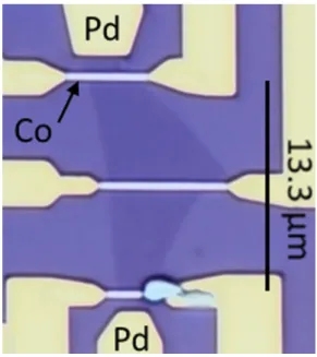
. Figure 2 shows a microscope image of the finished sample with five contacts (two Pd end contacts, three Co electrodes).

The measurements were performed in a cryostat with a three-dimensional (3D) vector magnet that consists of three superconducting magnetic coils, one large coil for the z axis and two identical smaller ones inside the z coil for the x and y fields. The xHanle experiment requires all three coils. The z and x magnets are used for zHanle and xHanle, while the y magnet is needed to switch the magnetic orientation of the electrodes from parallel (P) to antiparallel (AP). zHanle and xHanle were measured using different coils, so we checked if calibration errors, sample misalignment, and stray fields influence our data. We tested the calibration of the magnets with a Hall probe and also tested for magnetic hysteresis in a separate run. We found a hysteresis loop in the x and y magnets extending up to an applied field of 250 mT that can cause remanent fields of up to 2 mT. Therefore, unwanted stray fields of up to 2 mT can be present in the xy plane during the measurement and need to be taken into account when analyzing the data. We also checked for a misalignment of the sample and the magnets and found the possible misalignment angle to be below 3

. For a more detailed analysis of the magnetic setup, see the Supplemental Material [33].

FIG. 2. Optical micrograph of the graphene flake with contacts.

Cobalt electrodes (light gray) serve as ferromagnetic injectors and de- tectors. Pd electrodes (yellow) provide the spin-independent reference probes and also contact the Co electrodes for AMR measurements.

Figure 3 shows a back gate sweep of the graphene sheet resistance, with the Dirac point at V

= −2 V, indicating low extrinsic doping. For this measurement, the outermost electrodes were used to bias the sample and the voltage drop was detected between the Co electrodes that are later used as injector and detector for the spin experiments. The inset in Fig. 3 shows the differential resistance dR = dV /dI of the injector contact. The non-Ohmic behavior is an indication for high quality tunnel barriers.

Spin transport measurements were carried out in a nonlocal dc setup schematically shown in Fig. 1 at T = 100 K. Below this temperature, switching the electrodes into an antiparallel state produced inconsistent results, which can be attributed

-30 -20 -10 0 10 20 30

0 1k 2k 3k 4k

0.0 0.5 1.0 1.5 2.0

-0.2 -0.1 0.0 0.1 0.2 30.0k

35.0k 40.0k

dR [Ohm]

U [V]

Gate 30V

Sheet Resistance

R

[Ohm]

R[ O h m ]

Gate [V]

Spin valve Signal

FIG. 3. Gate dependence of the sheet resistance R

and the

nonlocal spin valve signal R

. The Dirac point is at −2 V. Inset

shows the differential resistance of the injector tunnel contact as a

function of current bias.

-0.10 -0.05 0.00 0.05 0.10 -0.6

-0.4 -0.2 0.0 0.2 0.4 0.6 0.8 1.0

R [Ohm]

AP

B

[T]

P

FIG. 4. Spin valve signal at V

= 12 V with illustrations to show the parallel (P) and antiparallel (AP) magnetic orientation of the electrodes. Distance of the injector and detector contacts was 13.3 μm with an injector current of 4 μA. The gray trace shows the preparation of the electrodes that was done at a higher sweep rate, which induces an offset because of the dc measurement setup.

to incomplete switching of the electrodes. Figure 4 shows a spin valve measurement at 100 K with properly switching electrodes and a spin valve signal of about R

= 1.2 .

The red graph in Fig. 3 displays the gate dependence of the spin valve signal at an injector current of 4 μA, used for all spin experiments here. The graph shows that the spin signal depends only weakly on V

. At negative injector bias there exists a regime where the back gate can be used to change the spin polarization of the injector current. This will be addressed elsewhere [34]. The experiments discussed in this paper were done at an injector bias where no change in the polarization of the injected spins occurs.

For the xHanle measurement, it is essential to prevent the Co electrodes from rotating their magnetization. This places a limit on the maximum magnetic field that can be applied in x direction. Narrow electrodes increase the magnetic shape anisotropy that keeps the magnetization aligned to the long axis. Additionally, a large distance between the contacts narrows the Hanle curve, reducing the required magnetic field.

It is common practice to use electrodes of different width to achieve different coercive fields needed to enable antiparallel switching of the electrodes. This is not practical for the xHanle experiment, as the electrodes should be as narrow as possible.

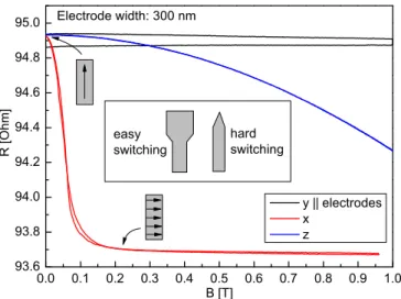
Instead, we achieve different coercive fields by shaping the tips of the electrodes, as shown in Fig. 5. A spatula-shaped tip reduces the coercive field, while preserving the magnetic stability with respect to perpendicular fields. Pointed tips, in contrast, increase the coercive field.

AMR measurements were carried out to see at what field values the Co electrodes rotate. According to the AMR data displayed in Fig. 5, at B

= 200 mT the electrodes are almost fully rotated into the x direction. This rotation is independent of the tip shape, so the AMR data are the same for all electrodes.

The peak width of the Hanle feature scales inversely with the

0.0 0.1 0.2 0.3 0.4 0.5 0.6 0.7 0.8 0.9 1.0 93.6

93.8 94.0 94.2 94.4 94.6 94.8 95.0

R [Ohm]

B [T]

y || electrodes x

z Electrode width: 300 nm

easy switching

hard switching

FIG. 5. AMR data of Co electrodes with the external field applied in x, y, and z directions. Illustrations show the orientation of the magnetization in the electrodes. Inset: Shape of the electrode tips for achieving different coercive fields while using the same width elsewhere.

travel time of the electrons. A long distance between injector and detector contacts is therefore needed in order to narrow the Hanle feature to a field range well below 200 mT. The xHanle measurements were done at magnetic fields only up to 25 mT to avoid rotation of the electrodes. Corresponding measurements are presented in the Supplemental Material [33].

For an injector-detector distance of 13.3 μm most of the Hanle feature was in that field range.

To analyze the influence of an external field in arbitrary di- rection, including stray field, misalignment, and the anisotropy of spin relaxation, we employ the diffusion equation for the spin density s [35]:

∂ s

∂t = s × ω + D ∂

s

∂x

− τ

s, (1) with

τ

=

⎛

⎝ τ

0 0 0 τ

0 0 0 τ

⎞

⎠ (2)

the anisotropic spin relaxation rate, D the spin diffusion constant, and ω the Larmor precession frequency vector, which is parallel to the magnetic field vector. While for Hanle experiments in isotropic media an analytical solution exists that is commonly used to fit the data [35], we resort to a numerical finite element solution using the commercial software package COMSOL to account for anisotropic spin lifetimes. A detailed description of the COMSOL model is provided in the Supplemental Material [33]. The simulated traces are then compared with experimental data of zHanle and xHanle. The parameters of the simulation are varied until the best possible match is obtained.

All Hanle measurements from which the spin lifetimes were extracted were performed using the outer Co electrodes, which have a distance of 13.3 μm, and an injector current of 4 μA.

At that distance, nonlocal spinvalve signals R

of 1.0–1.4

(depending on back gate voltage, see Fig. 3) could be achieved.

-20 -10 0 10 20 -0.6

-0.4 -0.2 0.0 0.2 0.4 0.6 0.8

R

[Ohm]

B

[mT]

zHanle xHanle Gate = 12 V

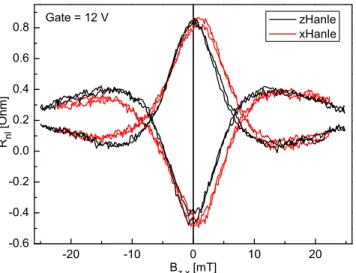
FIG. 6. Raw data of zHanle (black) and xHanle (red). Traces for both parallel and antiparallel magnetization were taken in both sweep directions.

Figure 6 shows the raw data of zHanle (black) and xHanle (red) at V

= 12 V. As can be seen, there is a distinctive difference between the traces, which will be discussed in more detail in Sec. III B. The remanent magnetization in the magnet setup leads to a slight shift of the xHanle curve and has to be included for fitting of both zHanle and xHanle. For example, the small stray field in x direction of about B

= 0.8 mT that causes the xHanle center peaks to be shifted slightly off zero field also causes a small reduction to the height of the center peak of the zHanle trace.

We will first analyze the zHanle data, which is the stan- dard characterization method in spin transport experiments.

Figure 7 shows the smoothed zHanle data (obtained by averag- ing the up and down sweep, subtracting the AP signal from the P signal and dividing by two). Due to the presence of unknown

-20 -10 0 10 20

-0.2 -0.1 0.0 0.1 0.2 0.3 0.4 0.5 0.6 0.7

Fit parameters:

D = 0.032 m²/s

xy= 850 ps stray field in y -1.0 mT stray field in x 0.8 mT

R

[Ohm]

B

[mT]

zHanle Data Fit

Gate = 12 V

FIG. 7. Smoothed data of zHanle (red trace) with fit for a stray field in B

= −1 mT and B

= 0.8 mT (blue dashed line). Smoothed data were obtained by averaging up and down sweep and subtracting P from AP sweep.

-10 -5 0 5 10

700 800 900 1000 1100 1200

180 200 220 240 260 280 300 320 340

D [cm ²/ s ]

xy[ps]

Gate [V]

spin-lifetime Parameters obtained from zHanle fitting

y stray field of -1 mT assumed for fitting

xy

diffusivity D

FIG. 8. In-plane spin-lifetime τ

and diffusivity D vs gate volt- age, extracted from fitting zHanle data with −1 mT stray field in y.

stray fields up to about 2 mT, we also included a B

field during the fitting procedure. The best match to the data was obtained with a stray field of B

= 0.8 mT and B

= −1 mT.

We fitted the zHanle data for several gate voltages and extracted the parameters for spin diffusivity and spin lifetime.

Figure 8 shows the fitted in-plane spin-lifetime τ

and diffusiv- ity D plotted against the back gate voltage. The spin lifetimes range from 730 to 1100 ps and show no correlation with the gate voltage. The spin diffusivity was a free parameter for the zHanle fit, giving 185 cm

/s as the lowest value at the Dirac point and 320 cm

/s as the highest value at V

= 12 V. We also extracted D

, the electron diffusivity, from the charge transport measurements shown in Fig. 3. Theses values are lower than the spin diffusivity (D

= 235 cm

/s at V

= 12 V). Using the electron diffusivity as a fixed parameter for zHanle fitting produced significantly worse fits, so this was disregarded. Note that due to the interdependence of the fitting parameters D and τ

the error bars and spread are rather large.

III. EXPERIMENTS ON ANISOTROPIC SPIN RELAXATION

A. Rotating the electrode magnetization

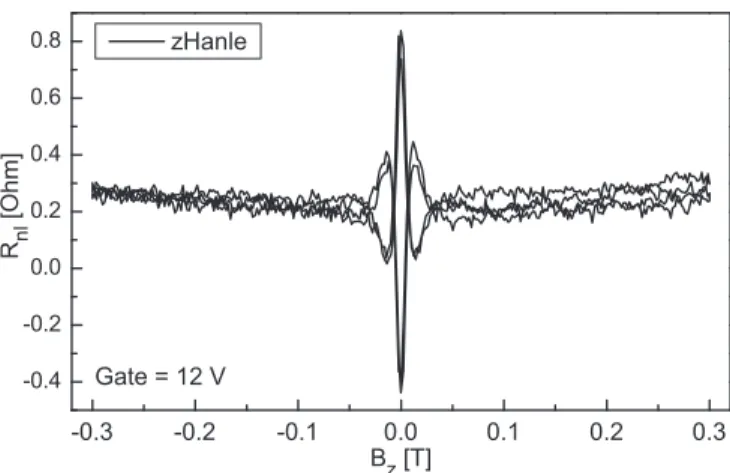
To check our setup, we performed zHanle and xHanle up to 300 mT. The slight symmetric increase of the background in the zHanle data shown in Fig. 9 can be attributed to the Co electrodes slowly rotating into the external field towards the z direction. We cannot fully rotate the electrodes towards z as our magnet is limited to 1 T. According to the AMR data in Fig. 5 however, 300 mT is enough to rotate the electrodes completely towards the x direction. In this case, the injected spins should remain in-plane and propagate without preces- sion. Since B

remains zero, no orbital magnetoresistance effects that could possibly influence the detected signal should be expected. Therefore, we expect that for complete rotation of the electrodes towards x , the xHanle signal fully recovers the zero field parallel state value.

The 300 mT xHanle is shown in Fig. 10 where the nonlocal signal at 300 mT is noticeably smaller than the zero field value.

Since at high B

the spin orientation remains in the graphene

-0.3 -0.2 -0.1 0.0 0.1 0.2 0.3 -0.4

-0.2 0.0 0.2 0.4 0.6 0.8

Gate = 12 V zHanle

R

[Ohm]

B

[T]

FIG. 9. zHanle measured up to 300 mT (raw data) to see the background at higher fields in parallel and antiparallel configuration.

plane all the time, no anisotropy of the spin lifetime is expected, so the signal loss must have a different origin. The most likely explanation for the signal loss is an imperfect magnetic alignment at the MgO-Co interfaces. Contrary to what the AMR data in Fig. 5 suggest, the interface magnetization is probably not yet fully aligned to the external field at 300 mT.

Spin injection and detection are sensitive to the interfaces of the electrodes, while AMR probes the bulk magnetization. It is known that a MgO-Co interface induces a strong magnetic coupling on the neighboring Co layers [36]. This coupling seems to make the interface magnetization more resistant to rotation than the bulk. More measurements that support this finding are discussed in the Supplemental Material [33].

We conclude that AMR data alone are not sufficient to characterize the electrodes for spin experiments. A magnetic coupling at the electrode interface also exists in other common material combinations like AlOx-Co [37,38]. This needs to be considered when using the electrode rotation technique to determine the spin-lifetime anisotropy. Hence, in addition to a

-0.3 -0.2 -0.1 0.0 0.1 0.2 0.3

-0.4 -0.2 0.0 0.2 0.4 0.6 0.8

Gate = 12 V xHanle

R

[Ohm]

B

[T]

Missing signal

FIG. 10. xHanle measured up to 300 mT (raw data) to see the rotation of the electrode magnetization. The upper double arrow indicates the difference between actual and expected signal at fields above 200 mT. The lower arrow indicates the missing data of the AP downsweep, because the high B

field flipped the electrodes back to P.

B

dependent background due to, e.g., the magnetoresistance of graphene [12,27], the interface magnetization is another possible source of error and has to be taken into account.

B. xHanle

The xHanle experiment requires no rotation of the elec- trodes and no high magnetic fields. To extract the spin-lifetime anisotropy, we first determine τ

from the zHanle data as detailed at the end of Sec. II. For xHanle, the magnetic field is aligned along the x axis (see Fig. 1), and the spins precess in the y-z plane. Therefore, the xHanle trace is sensitive not only to τ

, but also to τ

. For isotropic spin lifetimes, xHanle and zHanle should give identical results.

We now discuss in more detail the raw data of zHanle (black) and xHanle (red) at V

= 12 V shown in Fig. 6. Both traces are not identical, which could be caused by anisotropic spin lifetimes. Also, we notice a clear asymmetry with respect to B = 0 in the xHanle trace, not present in the zHanle data.

This could be due to sample misalignment in combination with stray fields. We simulated Hanle curves for this situation (see Supplemental Material for details [33]), and found that a sample rotation error of more than 12

would be required to produce an asymmetry of the observed magnitude. As this is far more than our estimated error of 3

, and the resulting trace does not match the shape of our data, we disregard this scenario.

The most likely cause for the asymmetry of the xHanle signal is then a magnetization misalignment of the electrodes.

Since the zHanle curve is not asymmetric, we conclude that the magnetization of the detector electrode contains a small z component in addition to the y component expected from shape anisotropy. Considering that the Co electrodes have a film thickness of 20 nm and are deposited on a near perfectly flat Si wafer, this tilted magnetization must be a local effect at the MgO-Co interface. It is know that a Co-MgO(100) interface induces a large perpendicular magnetic anisotropy in the neighboring Co layers [36]. This anisotropy is heavily dependent on crystallinity and oxidization state. Both param- eters are unknown.

To extract the data caused by the y and z components of the magnetization, we symmetrize and antisymmetrize the smoothed curves with respect to B = 0. The result is shown in Fig. 11. We get a large symmetric part that is the projection on the y component of the electrode magnetization and a smaller asymmetric part for the projection on the z component of the magnetization. For isotropic spin relaxation, the symmetric part would be identical to the zHanle as the zHanle is also projected on the y component of the magnetization. The remaining difference between zHanle and the symmetrized xHanle is now due to the anisotropy in spin relaxation. The symmetrized xHanle can be fitted very well with an anisotropy of ζ = 0.78. The antisymmetrized xHanle is fitted with the same parameters using only the scaling factor as a free variable.

The scaling factor can then be used to estimate the tilt angle

between injection and detection magnetization, which is ∼9

.

Summarizing this subsection, we note that the xHanle

experiment not only yielded the anisotropy ζ = 0.78, but

allowed us to detect a small degree of z magnetization in the

electrodes.

-20 -10 0 10 20 -0.2

-0.1 0.0 0.1 0.2 0.3 0.4 0.5 0.6 0.7

Gate = 12 V Fit parameters:

D = 0.032 m²/s

xy

= 850 ps stray field in y -1.0 mT

z

= 0.78*

z component scale factor: 0.15 R

[Ohm]

B

[mT]

zHanle xHanle, sym xHanle, antisym Fit

FIG. 11. Smoothed zHanle data (black) and symmetrized and antisymmetrized smoothed xHanle data (red and green), with fit traces for the xHanle (blue dashed lines).

C. Oblique spin precession

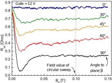
Finally, we performed the oblique spin precession exper- iment of Raes et al. [27] on our sample. As outlined in the Introduction, in this experiment an external field is applied at an angle β to the y axis (see also Fig. 1). When the field strength is varied at fixed β , we obtain a set of Hanle curves, shown in Fig. 12. At large enough field strength, the spin component perpendicular to the external field is fully dephased, leaving only the component parallel to the external field. The projection of the original spin direction onto the external field direction results in a cos β term in the signal. During diffusion to the detector electrode, the spins are subject also to the out-of-plane spin relaxation time, if β = 0. When entering the detector electrode, the spins are now projected onto the magnetization of the detector electrode, resulting in a further cos β term. For

0.00 0.05 0.10 0.15

0.0 0.1 0.2 0.3 0.4 0.5 0.6 0.7 0.8

0.9 Gate = 12 V

90°

60°

45°

R

[Ohm]

B [T]

Angle to plane

0°

30°

Field value of circular sweep

FIG. 12. Oblique spin precession traces at various inclination angles β of the magnetic field. The data at β = 90

correspond to the zHanle experiment.

0.0 0.2 0.4 0.6 0.8 1.0

0.0 0.2 0.4 0.6 0.8 1.0

Gate = 12 V

= 1

= 1.2

= 1.4

= 0.6 R

[norma lize d]

cos

(

)

= 0.8

FIG. 13. Sweep of the field angle β in the z-y plane at a constant field of 100 mT, plotted vs cos

β

to see the deviation from isotropic spin lifetimes that is linear in this plot. Colored lines show the simulated traces for various degrees of anisotropy.

isotropic spin relaxation, the nonlocal signal at the detector is therefore expected to follow a cos

β dependence, while ζ = 1 will lead to a deviation from that behavior. In Fig. 13 we plot the spin signal of a continuous sweep of the angle β at a fixed total external field of 100 mT. To account for differences between the actual electrode magnetization direction and the y-axis direction, the data in Fig. 13 are plotted vs cos

β

, where β

is the angle between external field and the electrode magnetization direction. The cos

scaling allows identifying any deviation from isotropic spin lifetimes easily. The colored lines show simulated traces for various degrees of anisotropy, applying Eq. (7) in Ref. [27] (see Supplemental Material for the full expression [33]). The magnetization direction in the injector and detector electrodes deviates from the y direction, which would be expected from shape anisotropy, due to rotation of the electrode magnetization in the external field and the partial z magnetization ascribed to the MgO/Co interface, which we detected in the xHanle experiment. This leads to correction terms that enter into the cos

β

term.

More details on fitting procedure and formula are discussed in the Supplemental Material [33]. As can be seen, the data fall roughly between the linear (isotropic) trace and the ζ = 0.8 trace. A fit of the data gives an anisotropy of ζ = 0.91.

Importantly, the z-magnetization component at the MgO/Co interface could only be detected in the xHanle experiment, but is crucial for the correct determination of ζ . Not accounting for the z component would have given an incorrect anisotropy of ζ = 1.08 [33]. The precision at which the tilt angle can be determined enters into the error bars of the oblique spin precession method.

IV. DISCUSSION

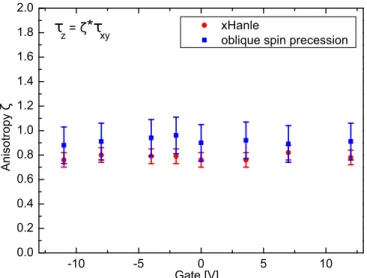
Figure 14 shows a comparison of the anisotropy extracted

from the oblique spin precession experiment and the xHanle

experiment. On average, the xHanle experiment gives an

anisotropy ζ slightly below 0.8, while the oblique spin

-10 -5 0 5 10 0.0

0.2 0.4 0.6 0.8 1.0 1.2 1.4 1.6 1.8 2.0

Anisotropy

Gate [V]

xHanle

oblique spin precession

z

= *

FIG. 14. Extracted anisotropy ratio ζ from xHanle data (red) and oblique spin precession data (blue) as a function of gate voltage.

precession gives ζ a bit larger than 0.9. There is no correlation to the gate voltage.

Our values for ζ extracted from the oblique spin precession data are still in the range observed in previous experiments [27], with ζ between ∼ 0.9 and ∼ 1.03. The values extracted from our xHanle data are slightly below that range.

The xHanle experiment measures the P and AP configura- tion, while the oblique spin precession experiment measures the P configuration only. First, this gives the xHanle experiment twice the amplitude over noise of the spin signal. Second, subtracting the AP from the P trace is a very reliable method to remove any background signal. The oblique spin precession experiment relies on normalization to remove any background.

The weakness of the oblique spin precession experiment is its sensitivity to the exact orientation of the electrode magnetization. On top of the permanent z component caused by the MgO-Co interface, the dynamic tilting because of the external field needs to be accounted for in the fit formula [33]. At our comparatively weak external field of 100 mT, the dynamic tilting correction is responsible for a shift in ζ by roughly − 0.07 and must be considered as a potential source of inaccuracy. Combined with the uncertainties related to determining the tilt angle of the permanent z component, this leads to significant error bars for ζ extracted from fitting the oblique spin precession data.

It follows from those arguments that the xHanle experiment is generally more precise than the oblique spin precession experiment and also more robust to nonideal conditions. As has been stated in Sec. III C, the permanent z tilt in the detector electrode was only identified because of the xHanle experiment, but the knowledge of its existence was crucial for correct interpretation of the oblique spin precession data. We therefore conclude that the anisotropy in our sample is slightly below ζ = 0.8 as per the xHanle data, which is within the error bars of our oblique spin precession experiment, but in contrast to previous claims of an isotropic spin relaxation time [27]. The disagreement between both results could be due to an overall higher spin relaxation rate in the experiment in Ref. [27].

For our sample, we assume that the spin relaxation stems from a mix of Rashba type spin-orbit fields that have a ζ of 0.5 and isotropic contributions like contact induced spin relaxation and resonant scattering by magnetic impurities. The individual relaxation rates are added to a total spin relaxation rate:

1 τ

= 1

τ

+ 1

τ

+ · · · . (3) Assuming the anisotropic contributions are only of the Rashba type, we can use this formula to separate anisotropic and isotropic contributions. That gives us τ

= 1.18 ns for the isotropic part and τ

= 3 ns and τ

= 1.5 ns for the anisotropic Rashba part.

The spin lifetime of the isotropic part is consistent with the model of resonant scattering by magnetic impurities, such as adsorbed hydrogen [19,20], assuming a low concentration of scatterers. The sample was measured at a pressure of ∼10 mbar, making a small concentration of hydrogen atoms or other species on the graphene surface plausible. This mechanism would exhibit a strong gate dependence when the energy approaches the resonance and no gate dependence at other energies. We do not see any significant gate dependence either in the spin lifetime or in the anisotropy within the gate range of our experiment. As the resonance can be outside of the energy range that we probed in our experiment (E

= 116 meV at V

= 12 V), this question could not be settled here.

Spin relaxation induced by the ferromagnetic electrodes, while still present, should be comparatively weak in our sample because of the high resistance area product of the contacts (cf.

Fig. 5 in Ref. [11]). The nonmagnetic Pd electrodes have a lower contact resistance of about 600 . They are outside the spin transport path, but less than one spin-flip length away, so we assume a small contribution to isotropic spin relaxation.

The local Rashba spin-orbit fields caused by the few adatoms are not significant enough to matter. For the global Rashba spin-orbit fields of the SiO

substrate, initially, Ertler et al. calculated the spin relaxation time to be at least a few μs with a maximum at the CNP [5]. Later, Van Tuan et al. obtained a few hundred ps with a minimum at the CNP [39]. More recent DFT calculations suggest a Rashba spin-orbit coupling of λ

in the range of tens of μeV for graphene on crystalline SiO

[40]. Using the D’yakonov-Perel’ mechanism, this works out to Rashba spin lifetime on the order of 1–10 ns, in agreement to our experimental data and in line with calculations by Cummings and Roche for clean graphene [41].

V. CONCLUSION

In conclusion, with the xHanle experiment we demonstrated

an additional way to measure the anisotropy of the spin lifetime

in graphene that we believe to be so far the most accurate

method. This tool can also be used to probe the spin relaxation

in similar 2D materials that have recently started to attract

interest like black phosphorus [42]. The data collected from

the xHanle experiment pointed to a nontrivial magnetization

of the contacts which is in line with the other experiments

we performed. We attribute this nontrivial magnetization to

a perpendicular magnetic anisotropy caused by the MgO-Co

interface. Not accounting for this magnetization would have

led to a false interpretation of the data from the oblique spin

precession experiment. Compared to the oblique spin pre- cession experiment, the xHanle is potentially more accurate, especially under nonideal conditions. The weakness of this ex- periment is that it needs to operate at low magnetic field values to prevent a rotation of the electrodes. At these low field values, possible stray fields from the remanent magnetization of the magnets are relevant enough to influence the measurement.

The graphene sample in this study showed an anisotropy in the spin lifetime of ζ slightly below 0.8 that was clearly visible in xHanle but could not be identified with this precision in the oblique spin precession experiment. We conclude that the spin relaxation mechanism in our sample is a combination of isotropic and anisotropic parts. We attribute the isotropic part to resonant scattering at adatoms and also contact induced

spin relaxation. The anisotropic part is due to Rashba spin orbit fields originating from the SiO

substrate.

ACKNOWLEDGMENTS

Financial support by the Deutsche Forschungsgemeinschaft (DFG) within the programs SFB 689 (project A7) and GRK 1570 is gratefully acknowledged, as well as financial support by the Elitenetzwerk Bayern. The authors would like to thank C. Back, G. Bayreuther, J. Fabian, D. Kochan, and K. Zollner for fruitful discussions. The authors would also like to thank F.

Volmer for his crucial advice on improving the quality of our MgO tunnel barriers and C. Strunk for the permission to use the UHV evaporator in his group.

[1] D. Huertas-Hernando, F. Guinea, and A. Brataas, Phys. Rev. B 74, 155426 (2006).

[2] W. Han, R. K. Kawakami, M. Gmitra, and J. Fabian, Nat.

Nanotech. 9, 794 (2014).

[3] M. Gmitra, S. Konschuh, C. Ertler, C. Ambrosch-Draxl, and J. Fabian, Phys. Rev. B 80, 235431 (2009).

[4] D. Kochan, S. Irmer, and J. Fabian, Phys. Rev. B 95, 165415 (2017).

[5] C. Ertler, S. Konschuh, M. Gmitra, and J. Fabian, Phys. Rev. B 80, 041405 (2009).

[6] B. Dóra, F. Murányi, and F. Simon, Europhys. Lett. 92, 17002 (2010).

[7] J.-S. Jeong, J. Shin, and H.-W. Lee, Phys. Rev. B 84, 195457 (2011).

[8] V. K. Dugaev, E. Y. Sherman, and J. Barnaś, Phys. Rev. B 83, 085306 (2011).

[9] D. Pesin and A. H. MacDonald, Nat. Mater. 11, 409 (2012).

[10] M. Drögeler, F. Volmer, M. Wolter, B. Terrés, K. Watanabe, T.

Taniguchi, G. Güntherodt, C. Stampfer, and B. Beschoten, Nano Lett. 14, 6050 (2014).

[11] M. Drögeler, C. Franzen, F. Volmer, T. Pohlmann, L. Banszerus, M. Wolter, K. Watanabe, T. Taniguchi, C. Stampfer, and B.

Beschoten, Nano Lett. 16(6), 3533 (2016).

[12] M. H. D. Guimarães, P. J. Zomer, J. Ingla-Aynés, J. C. Brant, N. Tombros, and B. J. van Wees, Phys. Rev. Lett. 113, 086602 (2014).

[13] S. Singh, J. Katoch, J. Xu, C. Tan, T. Zhu, W. Amamou, J. Hone, and R. Kawakami, Appl. Phys. Lett. 109, 122411 (2016).

[14] A. H. Castro Neto and F. Guinea, Phys. Rev. Lett. 103, 026804 (2009).

[15] F. Volmer, M. Drögeler, G. Güntherodt, C. Stampfer, and B.

Beschoten, Synth. Met. 210, 42 (2015).

[16] A. Avsar, I. J. Vera-Marun, J. Y. Tan, G. K. W. Koon, K.

Watanabe, T. Taniguchi, S. Adam, and B. Özyilmaz, NPG Asia Mater. 8, e274 (2016).

[17] M. Gurram, S. Omar, S. Zihlmann, P. Makk, C. Schönenberger, and B. J. van Wees, Phys. Rev. B 93, 115441 (2016).

[18] D. Huertas-Hernando, F. Guinea, and A. Brataas, Phys. Rev.

Lett. 103, 146801 (2009).

[19] D. Kochan, M. Gmitra, and J. Fabian, Phys. Rev. Lett. 112, 116602 (2014).

[20] D. Kochan, S. Irmer, M. Gmitra, and J. Fabian, Phys. Rev. Lett.

115, 196601 (2015).

[21] T. Maassen, I. J. Vera-Marun, M. H. D. Guimarães, and B. J. van Wees, Phys. Rev. B 86, 235408 (2012).

[22] F. Volmer, M. Drögeler, E. Maynicke, N. von den Driesch, M.

L. Boschen, G. Güntherodt, and B. Beschoten, Phys. Rev. B 88, 161405 (2013).

[23] F. Volmer, M. Drögeler, E. Maynicke, N. von den Driesch, M. L.

Boschen, G. Güntherodt, C. Stampfer, and B. Beschoten, Phys.

Rev. B 90, 165403 (2014).

[24] C. Józsa, T. Maassen, M. Popinciuc, P. J. Zomer, A. Veligura, H. T. Jonkman, and B. J. van Wees, Phys. Rev. B 80, 241403 (2009).

[25] P. J. Zomer, M. H. D. Guimarães, N. Tombros, and B. J. van Wees, Phys. Rev. B 86, 161416 (2012).

[26] A. G. Swartz, J.-R. Chen, K. M. McCreary, P. M. Odenthal, W.

Han, and R. K. Kawakami, Phys. Rev. B 87, 075455 (2013).

[27] B. Raes, J. E. Scheerder, M. V. Costache, F. Bonell, J. F. Sierra, J.

Cuppens, J. Van de Vondel, and S. O. Valenzuela, Nat. Commun.

7, 11444 (2016).

[28] N. Tombros, S. Tanabe, A. Veligura, C. Jozsa, M. Popinciuc, H. T. Jonkman, and B. J. van Wees, Phys. Rev. Lett. 101, 046601 (2008).

[29] B. Raes, A. W. Cummings, F. Bonell, M. V. Costache, J. F.

Sierra, S. Roche, and S. O. Valenzuela, Phys. Rev. B 95, 085403 (2017).

[30] L. A. Benítez, J. F. Sierra, W. Savero Torres, A. Arrighi, F. Bonell, M. V. Costache, and S. O. Valenzuela, Nat. Phys. 14, 303 (2018).

[31] T. S. Ghiasi, J. Ingla-Aynés, A. A. Kaverzin, and B. J. van Wees, Nano Lett. 17, 7528 (2017).

[32] G. Schmidt, D. Ferrand, L. W. Molenkamp, A. T. Filip, and B. J. van Wees, Phys. Rev. B 62, R4790 (2000).

[33] See Supplemental Material at http://link.aps.org/supplemental/

10.1103/PhysRevB.97.205439 for fabrication details, magnet setup, electrode magnetization, fitting procedure, and estimation of uncertainty.

[34] S. Ringer, M. Rosenauer, T. Völkl, M. Kadur, F. Hopperdietzel, D. Weiss, and J. Eroms, arXiv:1803.07911.

[35] J. Fabian, A. Matos-Abiague, C. Ertler, P. Stano, and I. Žutić, Acta Phys. Slovaca 57, 565 (2007).

[36] H. X. Yang, M. Chshiev, B. Dieny, J. H. Lee, A. Manchon, and

K. H. Shin, Phys. Rev. B 84, 054401 (2011).

[37] S. Monso, B. Rodmacq, S. Auffret, G. Casali, F. Fettar, B. Gilles, B. Dieny, and P. Boyer, Appl. Phys. Lett. 80, 4157 (2002).

[38] B. Rodmacq, S. Auffret, B. Dieny, S. Monso, and P. Boyer, J. Appl. Phys. 93, 7513 (2003).

[39] D. Van Tuan, F. Ortmann, A. W. Cummings, D. Soriano, and S. Roche, Sci. Rep. 6, 21046 (2016).

[40] K. Zollner and J. Fabian (private communication).

[41] A. W. Cummings and S. Roche, Phys. Rev. Lett. 116, 086602 (2016).

[42] A. Avsar, J. Y. Tan, M. Kurpas, M. Gmitra, K. Watanabe, T.

Taniguchi, J. Fabian, and B. Özyilmaz, Nat. Phys. 13, 888

(2017).