EVALUATION OF OBSERVATION NETWORK BENEFITS ON SHORT-TERM WEATHER FORECASTS FOR ENERGY-METEOROLOGY APPLICATIONS

EVALUATION OF OBSERVATION NETWORK BENEFITS ON SHORT-TERM WEATHER FORECASTS

FOR ENERGY-METEOROLOGY APPLICATIONS

I N A U G U R A L - D I S S E R T A T I O N ZUR

ERLANGUNG DES DOKTORGRADES

DER MATHEMATISCH-NATURWISSENSCHAFTLICHEN FAKULTÄT DER UNIVERSITÄT ZU KÖLN

vorgelegt von Paraskevi Vourlioti

aus Samos

Cologne, 2020

Berichterstatter: PD Dr. H. Elbern Prof. Dr. S. Crewell

Tag der mündlichen Prüfung: 03. Mai 2019

Abstract

The wind and solar energy sector relies on skillful Numerical Weather Prediction (NWPs) models to operate the power transmission grid resiliently. Moreover, accurate weather predictions are important for scheduling industrial power plants, but also for price fixing the energy stock market. One of the decisive factors for forecast skills is the quality of the initial state of the model, which may help to avoid or mitigate gross prediction failures repeatedly occurring during specific weather situations.

Through data assimilation, the best estimate of the atmospheric state is given by a combination of the forecasting model with observations, where the selection of measurements by type, location, and time in terms of their information value is essential. A monitoring tool, capable to quantitatively measure the capabilities of the observation network on the short-term forecast error is implemented and evaluated in this study for energy-meteorology applications.

The focus is placed on cases with exceptionally large prediction errors of solar and wind power, that challenge the weather centers and the Transmission System Operators (TSOs). To fulfill this request, a fortnight 01.-15.08.2014 that includes an exceptionally large error event on 09.08.2014 was selected. A satellite versus ground-based observation network configuration was chosen and a ranking list of the most beneficial observations was calculated. The Infrared Atmospheric Sounding Interferometer (IASI) onboard the Meteorological Operational Satellite (MetOp), as a precursor of a future sensor in a geostationary orbit, was evaluated against the classical Surface Synoptic Observations (SYNOP).

In terms of number of radiance channels per pixel, the bulk IASI data were found to contribute twice as much to the value of the forecasts in the case study compared to the SYNOP observations. Despite this, the normalized by number of observations results showed the SYNOP observations to be qualitatively superior. Especially the assimilation of the wind components were dominating the intraday forecast error reduction. The introduction in the assimilation of nine IASI water vapor channels added value to the model’s forecasts, in contrast to synoptic humidity observations.

The evaluation of the impact results per synoptic station location and IASI channel revealed both the most and least beneficial stations and channels.

With this method potentially all the observations for which data assimilation

is prepared to assimilate, can be evaluated and models can be configured with the

most favorable observations.

Kurzzusammenfassung

Die Wind und Solarenergieindustrie ist auf verlässliche Wettervorhersagemodelle angewiesen, um Übertragungsnetze sicher zu betreiben. Ferner sind genaue Wetter- vorhersagen wichtig, um Kraftwerkseinsätze effizient zu planen und am Energiemarkt realistische Preisbildung zu gewährleisten. Eine der entscheidenden Vorbedingun- gen guter Wettervorhersagen ist die Güte der Anfangswerte des Modells, die dazu beiträgt, Fälle schwerer Fehlvorhersagen zu vermeiden, die bei schwierigen Wetter- lagen auftreten können. Durch Datenassimilation ist eine optimale Schätzung des atmosphärischen Zustandes möglich, indem eine geeignete Kombination des Modells mit Beobachtungen vorgenommen wird. Das Verfahren, der Ort und die Zeit der Beobachtungen sind dabei wesentlich für die Güte.

In dieser Studie wird ein Auswerteverfahren eingerichtet und angewandt, welches in der Lage ist, die Güte von Beobachtungsnetzwerken und ihrer Messungen für energiemeteorologische Anwendungen quantitativ zu bewerten. Der Schwerpunkt liegt hierbei auf einer Analyse von größeren Fehlvorhersagen von Solar- und Winden- ergie, die Übertragungsnetzbetreiber aus einer Kombination von Wettervorhersagen ermittelt hatten. Dabei wurde eine zweiwöchige Episode vom 01. bis 15.8.2014 ausgewertet, die eine außergewöhnlich grobe Fehlvorhersage am 9.8.2014 enthält.

Hierzu wurde eine Kombination von Satellitendaten mit Bodenstationen ausgewertet und eine Bewertung der Beobachtungstypen nach ihrem Wert für eine Vorhersage- verbesserung durchgeführt. Das Infrared Atmospheric Sounding Interferometer (IASI) auf die Meteorologischer Operationssatellit (MetOp) wurde gegen klassische Boden- beobachtungen evaluiert.

Es wurde festgestellt, dass die IASI-Massendaten in Bezug auf die Anzahl der Strahlungskanäle pro Pixel doppelt so viel zum Wert der Prognosen in der Fallstudie beitragen wie die SYNOP-Beobachtungen. Trotzdem zeigten die nach Anzahl der Beobachtungen normalisierten Ergebnisse, dass die SYNOP-Beobachtungen qualitativ überlegen waren. Insbesondere erwies sich die Assimilation von Windkomponenten- daten als besonders wertvoll, die Vorhersagefehler innerhalb einer Tagesvorhersage zu reduzieren. Die zusätzliche Nutzung von neun IASI-Wasserdampfkanälen für die Assimilation erwies sich den synoptischen Feuchtebeobachtungen überlegen.

Die Auswertung der Beobachtungswirkung individueller Messungen oder Kanäle

kann mit dem hier entwickelten Verfahren besonders günstige oder ungünstige Beo-

bachtungskonfigurationen ermitteln, und zu möglichst effizienten Beobachtungsnetzen

insbesondere auch für energiemeteorologische Awendungen führen.

Contents

List of Figures iii

List of Tables vii

Acronyms ix

1 Introduction 1

2 Formulation of Forecast Sensitivity to Observations 5 3 Weather and Research Forecasting Model 11

3.1 Variational data assimilation in WRF model . . . 13

4 Experiment set-up 19 4.1 Observation configuration . . . 22

4.1.1 Infrared Atmospheric Sounding Interferometer . . . 23

4.1.2 Surface Synoptic Observations . . . 31

4.2 Assimilation of observations . . . 32

4.2.1 IASI assimilation . . . 37

4.2.2 SYNOP assimilation . . . 40

5 Observation impact results 43 5.1 Non-linear and linear forecast errors . . . 43

5.2 IASI and SYNOP observation impact . . . 46

5.2.1 Observation System Experiments . . . 52

5.3 Poor predictability cases . . . 54

5.3.1 Weather conditions . . . 59

5.4 Evaluation of the results . . . 64

5.4.1 Assimilation results . . . 64

5.4.2 Impact results . . . 69

5.4.3 Examination of observation impact . . . 83

6 Conclusions 89

A Appendix 93

A.1 FSO configuration at 18 UTC . . . 93

ii CONTENTS

A.2 Spatial distribution of observation impact for SYNOP wind measure- ments . . . 97 A.3 Model namelist configuration . . . 102

Bibliography 111

Acknowledgments 117

List of Figures

2.1 Schematic of FSO . . . . 5

3.1 Horizontal and vertical model grid configuration . . . 12

3.2 Vertical model levels . . . 12

3.3 WPS work-flow . . . 13

3.4 Flow-chart of WRFDA configuration . . . 14

3.5 Observation ingestion in WRFDA . . . 15

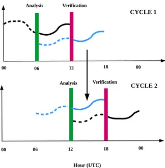
4.1 The cycling mode of the experiment set-up. . . . 19

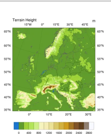
4.2 WRF domain used in the study. The terrain height is depicted in meters (m). . . 20

4.3 IASI on-board METOP and the first IASI/METOP-B spectrum on 24.10.2012 . . . 24

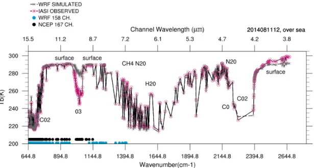
4.4 The IASI spectral channels . . . 27

4.5 IASI observation errors . . . 28

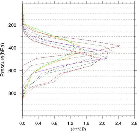
4.6 Emission weighting functions of nine water vapor channels of IASI . . 28

4.7 Emission weighting functions of IASI spectral channels . . . 30

4.8 SYNOP observations . . . 31

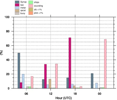
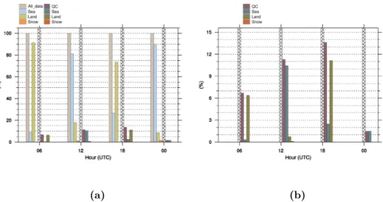
4.9 Assimilated observations types for the period 01.-15.08.2014 as a percentage of the total number of observations, at each assimilation hour . . . 33

4.10 Spatial domain coverage by IASI data . . . 35

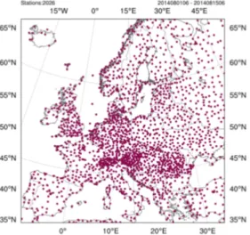
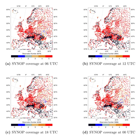
4.11 Spatial coverage by SYNOP data . . . 36

4.12 Bias correction scatter plots . . . 38

4.13 Percentage of IASI data that successfully passed quality control . . . 39

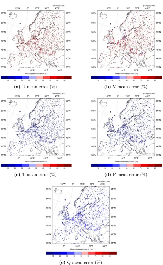
4.14 Percentage of SYNOP data that successfully passed quality control . 40 4.15 Mean SYNOP observation error for 01.-15.08.2018 . . . 41

5.1 Time series of the non-linear and the approximated linear error for 01.-15.08.2014. . . 44

5.2 Time series of linear versus non-linear forecast errors . . . 45

5.3 Time averaged error reduction by IASI and SYNOP . . . 46

5.4 Number of IASI and SYNOP data assimilated in the fortnight . . . . 47

5.5 Average error reduction, normalized by observation number . . . 48

5.7 Relative forecast error reduction . . . 48

iv LIST OF FIGURES

5.8 Time series of forecast error reduction by IASI and SYNOP, normalized by observation number . . . 49 5.9 Spatial distribution of SYNOP stations measuring pressure that had

the worst performance in the fortnight . . . 50 5.10 Spatial distribution and channel ranking list of the least beneficial

IASI assimilation in the fortnight . . . 51 5.11 Average forecast error calculated by OSEs . . . 53 5.12 Time series (01.-15.08.2014) of day-ahead forecasts and actual total

power values . . . 54 5.13 Time series (01.-15.08.2014) of day-ahead forecasts and actual total

power values at the four assimilation hours . . . 55 5.14 Time series of RMSE and MAE . . . 56 5.15 RMSE per hour (00, 06, 12, 18 UTC) for 01.-15.082014. . . 56 5.16 Time series of days-ahead forecasts and actual total power values for

wind power, on days of large error events . . . 57 5.17 Time series of days-ahead forecasts and actual total power values for

wind power, on days of large error events. . . . 57 5.18 Geopotential height in decametres at 500 hPa and sea level pressure

plots, for the poor predictability cases . . . 59 5.19 Surface analyses by DWD and SEVIRI imagery on days of poor

predictability cases(a) . . . 61 5.20 Surface analyses by DWD and SEVIRI imagery on days of poor

predictability cases(b) . . . 62 5.21 Time series of innovation and analysis residuals, for assimilation of

SYNOP data . . . 66 5.22 Time series of innovation and analysis residuals, for assimilation of

IASI data(a) . . . 67 5.23 Time series of innovation and analysis residuals, for assimilation of

IASI data(b) . . . 68 5.24 Observation impact per assimilation hour for the European domain . 70 5.25 Relative forecast error reduction by assimilation of IASI and SYNOP 71 5.26 Relative forecast error reduction by assimilation of SYNOP measure-

ments and IASI spectral channels . . . 72 5.27 Spatial distribution and channel ranking list of the most beneficial

SYNOP and IASI observations on 09.08, 06 UTC . . . 74 5.28 Spatial distribution and channel ranking list of the most beneficial

SYNOP and IASI observations 11.08., 06 UTC . . . 75 5.29 Spatial distribution and channel ranking list of the most beneficial

SYNOP and IASI observations on 03.08., 12 UTC . . . 77 5.30 Spatial distribution and channel ranking list of the most beneficial

SYNOP and IASI observations on 04.08.,12 UTC . . . 78 5.31 Spatial distribution and channel ranking list of the most beneficial

SYNOP and IASI observations on 09.08., 12 UTC . . . 79 5.32 Spatial distribution and channel ranking list of the most beneficial

SYNOP and IASI observations on 10.08., 12 UTC . . . 80

LIST OF FIGURES v

5.33 Spatial distribution and channel ranking list of the most beneficial SYNOP and IASI observations on 11.08., 12 UTC . . . 81 5.34 Spatial distribution and channel ranking list of the most beneficial

SYNOP and IASI observations on 13.08., 12 UTC . . . 82 5.35 Scatter plots of observation impact of SYNOP variables and their

corresponding innovation vector. . . 84 5.36 Scatter plots of observation impact of IASI spectral channels and their

corresponding innovation vector. . . 86 A.1 FSO configuration at 18 UTC . . . 94 A.2 FSO configuration at 12 UTC . . . 95 A.3 Impact of SYNOP stations measuring wind (assimilation of meridional

V) on the 6-hour forecast, for assimilation hour 06 UTC and for all poor predictability cases. . . 98 A.4 Impact of SYNOP stations measuring wind (assimilation of meridional

V) on the 6-hour forecast, for assimilation hour 12 UTC and for all poor predictability cases. . . 99 A.5 Impact of SYNOP stations measuring wind (assimilation of zonal U)

on the 6-hour forecast, for assimilation hour 06 UTC and for all poor predictability cases. . . 100 A.6 Impact of SYNOP stations measuring wind (assimilation of zonal U)

on the 6-hour forecast, for assimilation hour 12 UTC and for all poor

predictability cases. . . 101

List of Tables

2.1 Forecast error approximations . . . . 9

4.1 WRF model configuration . . . 20

4.2 Computational resources on JURECA. One FSO cycle demands the execution of WRF forward model, assimilation and adjoint model. The calculation of the impact is done with the help of the WRF assimilation model. . . 21

4.3 Spectral range given in units of cm

and µm along with the corre- sponding IASI application (Chalon et al. [2001]). . . 25

4.4 Observation types assimilated to produce the reference analysis in the FSO scheme . . . 32

5.1 Dates with highest RMSE and MAE scores for wind and solar power. 56 5.2 Relative forecast error in percentage for days with the largest RMSE and MAE scores. . . 58

A.1 WRF namelist for the forward runs. . . 103

A.2 WRFVAR namelist for the assimilation runs. . . 104

A.3 WRFPLUS namelist for the adjoint runs. . . 106

A.4 WRFVAR namelist for impact calculation runs. . . 107

Acronyms

AFWA Air Force Weather Agency

AIRS Atmospheric Infrared Sounder

ALADIN Aire Limitée Adaptation dynamique Développement InterNa- tional

AMSU-A Advanced Microwave Sounding Unit-A

ARPEGE Action de Recherche Petite Echelle Grande Echelle

ARW Advanced Research WRF

ASCAT Advanced Scatterometer

ATOVS Advanced TIROS Operational Vertical Sounder AVHRR Advanced Very High Resolution Radiometer

CG Conjugate Gradient

CRTM Community Radiative Transfer Model

DWD Deutscher WetterDienst

EUMETSAT European Organization for the Exploitation of Meteorological Satellites

ECMWF European Centre for Medium-Range Weather Forecasts EFOV Effective Field Of View

EPS EUMETSAT Polar System

FAA Federal Aviation Administration

FASTEX Fronts and Atlantic Storm-Track EXperiment

FEC Forecast Error Contribution

FOV Field Of View

FSL Forecast Systems Laboratory

FSO Forecast Sensitivity to Observations GDAS Global Data Assimilation System

GFS Global Forecasting System

GMAO Global Modeling and Assimilation Office GNSS Global Navigation Satellite System

GOES Geostationary Operational Environmental Satellite GRAS Global Receiver for Atmospheric Sounding

GTS Global Telecommunications System

x Acronyms

IASI Infrared Atmospheric Sounding Interferomenter

IR Infrared

IRS Infrared Sounder

JCSDA Joint Center for Satellite Data Assimilation

JSC Jülich Supercomputing Center

JURECA Jülich Research on Exascale Cluster Architectures

MAE Mean Absolute Error

METAR Meteorological Aerodrome Report MetOp Meteorological Operational Satellite

MPI Message Passing Interface

MSG MeteoSat Second Generation

MTG MeteoSat Third Generation

NAE North Atlantic and European model

NASA National Aeronautics and Space Administration NAVDAS NRL Atmospheric Variational Data Assimilation NCAR National Center for Atmospheric Research NCEP National Centers for Environmental Prediction

NESDIS National Environmental Satellite Data and Information Ser- vice

NMC National Meteorological Center

NOGAPS Nany Operational Global Atmospheric Prediction System

NRL Naval Research Laboratory

NWP Numerical Weather Prediction

OMA Observation Minus Analysis

OMB Observation Minus Background

OSE Observation System Experiment

OSSE Observation System Simulation Experiments

PREPBUFR Prepared Binary Universal Form for the Representation of meteorological data

RMSE Root Mean Square Error

RTE Radiative Transfer Equation

SEVIRI Spinning Enhanced Visible and Infrared Imager

SFR Spectral Response Function

SV Singular Vectors

SSM/I Special Sensor Microwave Image SYNOP Surface Synoptic Observations

TSO Transmission System Operators

TCW Total Cloud Water

VarBC Variational Bias Correction

Acronyms xi

WMO World Meteorological Organization

WPS WRF Preprocessing System

WRF Weather amd Research Forecast

WRFDA WRF Data Assimilation System

3DVAR 3 Dimentional Variational Assimilation

4DVAR 4 Dimentional Variational Assimilation

Chapter 1 Introduction

With a target of supplying 27% share of energy consumption from renewable sources by 2030 (European Parliament [2014]), the research field of energy meteorology, comprising wind and solar energy, is flourishing. Accurate short-term wind and solar power forecasts are vital for maintaining power grid stability, scheduling the power plants but also for the energy stock market (Kleissl [2013]). The day-ahead solar and wind power forecasts are typically provided by NWPs, which simulate the physical processes of the atmosphere based on the primitive equations.

The key to the accurate day-ahead solar and wind power forecasts lies in the performance of the NWPs. Some of the main drivers of the performance are the measurements availability for the initial state, the physical parameterizations and the computational resources to compute with high spatial resolutions (Kleissl [2013]).

Finding the optimal way to initialize a model brings into focus the research field of data assimilation. Data assimilation is the technique that combines observations and NWPs along with their corresponding errors to provide the best estimate of the atmospheric state, called the analysis (Kalnay [2003]). The analysis can be used in various ways, including initialization, studying the climate through reanalyses, examining individual components of the existing observation network by conducting Observation System Experiments (OSEs), and predicting the potential impact of new components of the observation network via Observation System Simulation Experiments (OSSEs) (Barker et al. [2003]).

Energy meteorology and data assimilation can be combined in an fruitful way for optimal observation network configuration, in terms of wind and solar power generated energy prediction. In particular, the information gain by the different types of assimilated observations can be assessed and monitored with the help of well defined properties of the assimilation system. The relative impact of the ob- servation network on the short-term forecast can then be investigated in terms of spatio-temporal configuration.

In the frame of data assimilation, the impact of observation data sets on the

quality of the forecast is traditionally estimated by the OSEs. These experiments

demand the removal of subsets of observations from a data assimilation system and

the resulting forecast is compared against a control set that includes all observations

(Daley [1993]). But, because of their computational expense, they usually involve

2 Introduction

only a small number of independent experiments (Gelaro and Zhu [2009]). In recent years a new algorithm relying on the adjoint (i.e. mathematical transpose) properties of the data assimilation system has been developed and measures the response of the forecast error to all perturbations, including all available observations in the experiment. This algorithm does not only include all the observations in the system, leaving the gain matrix untouched (Cardinali [2009]) but is also computationally cheap, allowing a monitoring aspect of the performance of the observation network relative to weather conditions. This advanced and sophisticated tool for estimating the data impact on the forecasting system is called Forecast Sensitivity to Obser- vations (FSO)(Langland and Baker [2004]). FSO answers the question where and which observations should be placed (by the sensitivity gradients) and how much each observation (by variable or by instrument) has contributed to improve the forecast. The latter can be viewed as complementing the OSEs and the answer to the former falls in the targeted observations research.

The concept of targeted observations addresses the question of identifying in advance, regions where additional observations would improve the forecast. For instance, Langland et al. [1999] assessed the impact of observations placed in real time in regions identified apriori, as target regions, by the most rapidly growing singular vectors (SVs) of the linearized model in the context of the Fronts and Atlantic Storm-Track EXperiment (FASTEX) during January and February of 1997.

They employed dropsonde and satellite wind data on the sensitive locations and demonstrated improved 24 hour forecast skill with this technique. More specific, the SV method defines a matrix problem, consisting of the tangent and the adjoint model (transpose of the linearized forecast model) along with a scaling matrix, which is usually an energy norm (Baker and Daley [2000]). The SVs of the adjoint model maximize the growth of the perturbation energy. Studies of Gelaro et al. [1998] and Palmer et al. [1998] supported the applicability of the total energy norm for studying the atmospheric predictability within the time scales of NWPs. They demonstrated this by showing that the spectra of singular values are dominant in the wavenumber band for which the analysis error variance is relative small (Palmer et al. [1998]).

The SVs approach for the targeted observations is based on the fact that corrections to initial conditions of the forecasts, result in improved forecast skills (Rabier et al.

[1996]). The success of the SVs is attributed to the fraction of the analysis error that projects into the leading SVs. The growth of this component of the analysis error can dominate the forecast error (Gelaro et al. [1999]). Both the SV and the adjoint sensitivity method are related in a mathematical sense. Analyzing the FASTEX campaign they pinpointed to similar sensitive areas.

Following the introduction of the FSO tool, many weather centers have extended

their data assimilation systems by FSO to estimate the distinct value of various data

sets on the short term forecast. For example, the Naval Research Laboratory and

National Aeronautics and Space Administration/Global Modeling and assimilation

Office (NASA/GMAO) have adopted the scheme on an operational basis to monitor

the observation network assimilated in their models (Kalnay et al. [2012]).

3

Langland and Baker [2004], calculated the 24 hour global forecast error of the Navy Operational Global Atmospheric Prediction System (NOGAPS) during June and December 2002. They used the Naval Research Laboratory (NRL) Atmospheric Variational Data Assimilation (NAVDAS) system to perform the 3 Dimensional Variational Assimilation (3DVAR) of space borne observations (e.g. from the Geo- stationary Operational Environmental Satellite (GOES) and the Advanced TIROS Operational Vertical Sounder (ATOVS)) as well as surface data from ships, buoys and other in-situ devices. It was found that 60% of the global error reduction was due to observations below 500 hPa and they revealed a strong correlation between observation impact and cloud cover at observation location. For instance, in locations with 80 % cloud cover the impact of rawinsonde temperature observation was found to be 1,5 times larger than in locations with 20 % cloud cover. Two explanations were given for this finding, the first one referring to the study of McNally [2002]

claiming cloudy regions to be more sensitive to analysis errors and the second one arguing that in cloudy regions fewer observation are available for assimilation (e.q due to quality control) and thus are given more weight in the assimilation procedure.

These findings support the concept of adding information (i.e observations) into cloudy regions could be a means to improve the forecast skill.

Joo et al. [2013], studied the value of space borne observations on the 24 hour forecast using the FSO scheme, adapted for the Met Office global NWP model and the 4 Dimensional Variational Assimilation (4DVAR) assimilation system. The experiment was conducted from 22.08. to 29.09 2010. Compared to ground based observations, satellite data were found to account for 64 % of the forecast error reduction. Moreover microwave and hyperspectral infrared soundings had the largest total impacts. For satellite platforms, MetOp-A had the largest impact. This was attributed to four sensors: IASI (Infrared Atmospheric Sounding Interferometer), GNSS (Global Navigation Satellite System), Global Receiver for Atmospheric Sound- ing (GRAS) and the Advanced Scatterometer (ASCAT). A major source of forecast improvement from a ground based observations type were the assimilated Meteoro- logical Aerodrome Reports (METAR) (Joo et al. [2013]). The study did not account for varying atmospheric conditions but concluded that FSO can be exploited in this manner.

Jung et al. [2013], applied the FSO scheme in East Asia and the western Pacific

for the 2008 typhoon season (16.08. - 01.10.2008). They were the first to examine the

capability of the scheme in the limited area Weather Research and Forecasting (WRF)

model and the sensitivity to the error covariance parameters. They used the 3DVAR

assimilation system with a 45 kilometer resolution, and calculated the 6-hour forecast

impact from different types of observations including ground based synoptic reports

and satellite observations like the Advanced Microwave Sounding Unit-A (AMSU-A),

but no infrared observations. They discovered that for this application the fraction

of beneficial observations was higher (60 % -70 % of observation were beneficial) than

reported in previous studies and that in the ranking list, the synoptic reports were

the most beneficial after the satellite AMSU-A observations. The impact of satellite

measured temperature brightness was found to be one order of magnitude greater

than the one from conventional observations, as the magnitude is also proportional

4 Introduction

to the observation number. As for the conventional observations, in agreement with the World Meteorological Organization (WMO) Andersson [2008], the impact of momentum variables was found to be greater than those of moisture and mass. Their results were also evaluated successfully with OSEs.

This study aims to apply and evaluate the FSO algorithm for the specific needs of energy meteorology, where skillful short-term forecasts are vital. Emphasis should be placed for episodes of exceptionally poor predictability. That is for cases where even weather centers collectively produced erroneous forecasts, which resulted in grid management difficulties and ruined power trading revenues. A ranking list of the most valuable assimilated observations for the short-term forecast should be identified, indicating the values of observation types and individual measurements. For the satellite data, particular attention should be given to sensors that are expected to play a leading role in the future. This request leads to the evaluation of IASI, onboard MetOp, serving as a precursor to the Infrared Sounder (IRS) on MeteoSat Third Generation (MTG) (EUMETSAT [2019]). The classical in-situ synoptic reports, should be evaluated against the prominent satellite data.

The formulation of the algorithm is described in Chapter 2. In Chapter 3, the NWP model and the radiative transfer model utilized for this study are presented.

The configuration of the experiment, including experiment set-up and information on

the examined observations are given in Chapter 4. Next, the aggregated results for

the examined time span, the OSE experiments and the focus on low solar and wind

power predictability days are given in Chapter 5. The conclusions and discussion of

the results are presented in Chapter 6.

Chapter 2

Formulation of Forecast Sensitivity to Observations

Forecast Sensitivity to Observations (FSO) is an adjoint based technique that allows the calculation of the observations impact on the assimilation result, commonly termed analysis, at each distinct assimilation cycle. Subsequently, an analysis as defined in section (Section 3.1) is calculated first. The goal of FSO is then to quantitatively measure the forecast error reduction caused by each distinct observation or observation type. The configuration of FSO is depicted on Fig. 2.1, where a 3DVAR analysis is calculated at time t

. In the next paragraphs, FSO will be formulated (Langland and Baker [2004]) by unraveling this configuration, to end up with the core of the FSO equation.

t

t

t

F o re c a st e rr o r (J /k g )

Observations

x

x

e

x

e

Figure 2.1: Schematic of FSO. Two forecasts, (x

, x

), are initiated with a difference of six hours and evaluated at verification time after six hours (t

).

The error measure is defined upon verification time as the difference of the two forecasts

from the reference analysis x

.

6 Formulation of Forecast Sensitivity to Observations

After the assimilation is performed at t

, two forecasts are initiated: one starting from the analysis time and an other one from a model run initiated at t

. Both end at t

. The forecast starting at t

, serves as background information for the assimilation at t

. This means that at t

, the only difference between the two forecasts is the information gained from the observations, which are included in the forecast initiated from the analysis.

At this time step (t

), an overall scalar forecast error e has to be defined for which the impact of observations will be calculated. The dry total energy norm, in units of J/Kg,

e = 1 2

ZZ Z

Σ

[u

+ v

+ ( g

N Θ )

Θ

+ ( 1

ρc

)

p

] dΣ (2.1) is a suitable and commonly used choice as it consists of the most relevant model variables (namely wind speed, temperature and pressure) (Rabier et al. [1996]). The energy norm is used to calculate the forecast error cost function or forecast response.

It allows the comparison of different types of measurements and physical parameters as wind and temperature by one scale. The first part of (Eq. (2.1)) specifies the kinetic energy and the second the available potential energy. More specific, u

, v

, Θ

, p

are perturbations of zonal wind, meridional wind, potential temperature and pressure, respectively. The coefficients are, Θ which is the potential temperature, ρ is the density, c

is the speed of sound and N denotes the Brunt-Vaisala frequency.

The dΣ denotes the integration over the domain’s three dimensions x, y and z.

Then, two cost functions J

and J

that measure the contribution to the forecast errors e

and e

from the two forecasts x

, x

are defined as,

J

= 1

2 e

(2.2)

J

= 1

2 e

(2.3)

where,

e

= (x

− x

)

C(x

− x

), (2.4) and

e

= (x

− x

)

C(x

− x

). (2.5) The forecast errors e

and e

are quadratic error measures of the forecasts initiated from the analysis x

and the earlier forecast x

with respect to the reference state x

. The reference state is usually an analysis provided at the verification time t

by the same model that provides the forward runs.

The superscripts in the equations refer to the corresponding times as illustrated in Fig. 2.1 and C is a diagonal matrix containing the weights according to the total dry energy norm.

The non-linear forecast error reduction can then be defined as the difference of

the two quadratic error measures ∆e

= e

− e

and can be exactly calculated using

(Eq. (2.4)) and (2.5). This formulation provides a simple plus/minus configuration,

7

where negative values would imply forecast improvement due to assimilation as the forecast from the analysis would be closer to the reference than the simple forecast.

Similarly positive values of the non- linear forecast error would imply degradation of the forecast due to assimilation. In order to establish a relation between forecast error at forecast and assimilation time, the adjoint model (transposed of the linearized version of the forecast model) is utilized. An approximation of ∆e

is sought with the use of adjoint sensitivity gradients. To achieve this, ∆e

can be expressed with the use of equations (Eq. (2.2)) and (2.3). The gradients of the cost function

∂J

/∂x

and∂J

/∂x

are given by:

∂ J

/∂x

= C(x

− x

) (2.6)

∂J

/∂x

= C(x

− x

) (2.7) These gradients serve as input information to the adjoint model, starting from time t

back to the assimilation time at t

. Two adjoint model runs are performed, from the forecast time t

to assimilation time t

.

The adjoint model maps the sensitivity of the forecast response with respect to the forecast control vector, ∂ J

/∂x

and ∂ J

/∂x

, into the sensitivity of the forecast response with respect to the initial conditions, ∂J

/∂x

and ∂J

/∂x

, linearized along the forecast trajectories. The resulting gradients, show locations, where changes to the initial conditions have the largest impact on the forecast error.

The sensitivity of the forecast error to initial humidity conditions are obtained by the adjoint of the linearized moist physical processes as a secondary effect (Janisková and Cardinali [2017]).

The sensitivity of the forecast response to the observations, ∂J/∂y

, can be derived from the sensitivity of the forecast response to the initial conditions by using the rule of chain,

∂J

∂y

= ∂J

∂x

∂ x

∂ y

(2.8)

where the gradient ∂x

/∂y

= K

, provides the sensitivity of the analysis system to the observations. The calculation of the adjoint of the data assimilation system is a computationally demanding task, as the inverse of the analysis error covariance matrix, A

, has to be approximated (Daley [1993]).

K

= R

HA

, (2.9)

where H is the observation or forward operator that maps from model to observation space and R is the observation error covariance matrix. The Lanczos algorithm that calculates the converged eigenvalues lying in the Krylov subspace (Van der Vorst [2003]) is used to approximate the inverse of A. To accomplish this, the minimization algorithm is switched from Conjugate Gradient (CG) to Lanczos and it can be proven that the error associated with the variation solution is given by the inverse of the Hessian matrix (second derivative of the 3DVAR cost function):

A

= ( ∂

J

∂

x ) = B

+ H

R

H. (2.10)

8 Formulation of Forecast Sensitivity to Observations

Eq. (2.10) states that the precision of the analysis error covariance is equal to the sum of the precision of the background information and the observations passed through the observation operator (Zou et al. [1997]). Now, Eq. (2.8) becomes:

∂J

∂y

= K

∂ J

∂x

(2.11)

for the sensitivity stemming from the analysis x

and

∂J

∂y

= K

∂ J

∂x

(2.12)

for the sensitivity stemming from the forecast x

. Similarly to the sensitivity of the response function to the initial conditions, the sensitivity of the response function to the observations indicates locations where small changes to the observations have the greatest impact on the forecast error. Baker and Daley [2000] derived the sensitivity of the forecast response to initial conditions at time t

as:

∂J

∂ x

= ∂J

∂x

+ ∂J

∂x

(2.13)

The non-linear error can then be expressed in terms of gradients at forecast time.

∆e

= h(x

− x

)

, ( ∂J

∂ x

+ ∂ J

∂x

)i (2.14) The connection between the forecast error at forecast time with the error at as- similation time can now be made. The approximation of ∆e

can be written as:

δe

= hδx

, ( ∂ J

∂ x

+ ∂J

∂x

)i (2.15)

where δx

is the analysis increment and δe

becomes:

δe

= hK(y − Hx

), ( ∂J

∂x

+ ∂ J

∂ x

)i (2.16) δe

is not an exact calculation as ∆e

, because the sensitivity gradients are calculated with the use of the adjoint model. Using the adjoint property,

δe

= h(y − Hx

), K

( ∂J

∂x

+ ∂J

∂x

)i (2.17)

the approximation can be written as

δe

= h(y − Hx

), ∂J

∂y

i (2.18)

The final step to quantitatively estimate the observation impact in the forecast

error is to calculate the inner product of the sensitivity of the response function to

9

observation and the innovation vector d (see Eq. (3.2)). This means the greater the innovation vector, the greater the impact. The Forecast Error Contribution (FEC) by the assimilation of observations or observation impact is defined as:

δe

= hd, ∂J

∂ y

i. (2.19)

According to Gelaro et al. [2007], various orders of approximation of observation impact can be derived with the use of Taylor expansion. More specific, the acquired variations are presented in Table 2.1.

Table 2.1: The first (δe1), second (δe2) and third (δe3) order Taylor approximations.

δe4 and δe5 are augmented versions of the third order approximation.

Measure Formula

∆e (x

− x

)

C(x

− x

) − (x

− x

)

C(x

− x

) δe1 2(x

− x

)

K

M

C(x

− x

)

δe2 (x

− x

)

[M

C(x

− x

) + M

C(x

− x

)]

δe3 (x

+ x

)

[M

C(x

− x

) + M

C(x

− x

)]

δe4 (x

− x

)

[M

C(x

− x

) + M

C(x

− x

)]

δe5 (x

− x

)

[M

C(x

− x

) + M

C(x

− x

)]

Here, M

=

t0+∆t a

∂x^ta⁰

& M

=

t0+∆t f

∂x^t_f⁰

are the resolvent matrices of the tangent linear version of the WRF model and M

, M

are the adjoint WRF matrices, that transfer the sensitivity gradients from forecast time to assimilation time. For example, δe5 differs from δe4 only by the choice of the adjoint matrix M

which replaces the adjoint matrix M

. This means that for δe5 the linearization is done along the trajectory of the simple forecast x

instead of the forecast initiated from the analysis x

.

The augmented version of the error approximation was adopted for this study, δe4 = (x

− x

)

[M

C(x

− x

) + M

C(x

− x

)]. (2.20) This version was found by Gelaro et al. [2007] to be a better approximation to the non-linear error ∆e compared to the other approximations (δe1, δe2, δe3, δe5).

This was achieved by exactly calculating the values of the non-linear error ∆e and its approximations according to the formulas in Table 2.1. This result was also confirmed in this study, where for some selected days the relative error between ∆e and its approximations was exactly calculated for the European domain.

In order to verify the results qualitatively, the traditional but rather computational

expensive OSEs experiments were performed for the targeted domain, time span,

and observations. The details of how the experiments were conducted and the results

can be found in Section 5.2.1.

Chapter 3

Weather and Research Forecasting Model

The WRF model is a state of the art numerical weather prediction system for atmospheric research (Skamarock et al. [2008]). The development of WRF was a collective effort from a number of institutions, namely the National Center for Atmospheric Research (NCAR), the National Centers for Environmental Prediction (NCEP), Forecast Systems Laboratory (FSL), Air Force Weather Agency (AFWA),

Federal Aviation Administration (FAA) at the late 90

s. In this work the WRF-ARW model (Advanced Research WRF) is utilized, developed from NCAR’s Mesoscale and Microscale Meteorology Laboratory.

The system consists of the dynamical solver, dynamic/numeric options, physics

schemes and the data assimilation component. Specifically the ARW solves fully

compressible, non-hydrostatic Euler equations (advection, Coriolis, buoyancy etc)

and the prognostic variables include velocity components in Cartesian coordinates,

perturbation temperature, perturbation geopotential and perturbation surface of

dry air. Optionally, TKE (Turbulent Kinetic Energy) and scalars such as cloud

water/ice mixing ratio, water vapor mixing ratio and chemical species and traces

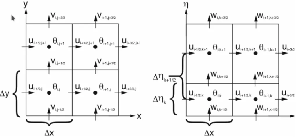
can be also prognosed. The used grid is the Arakawa-C grid staggering stensil as

shown in Fig. 3.1.

12 Weather and Research Forecasting Model

Figure 3.1: On the left, the horizontal and on the right the vertical Arakawa C-grid configuration is depicted. At the center of the left face are the zonal velocities in X direction and at the center of the front face are the meridional velocities in Y direction. At the center of the bottom face are the vertical W points in Z direction and at the center are the Θ points (Skamarock et al. [2008]).

Scalar state variables (thermodynamical variables such as potential temperature and pressure) are calculated at Θ points and the horizontal wind components are stored in X stagger (u) and Y stagger (v) dynamics. The vertical wind component w is stored in the Z stagger dynamics at half levels. As can be seen in Fig. 3.2, the vertical coordinate is not evenly spaced because it is a terrain following, dry hydrostatic pressure with a constant pressure p

at the top of the model.

Figure 3.2: The equations in ARW are formulated using the terrain following hydrostatic- pressure defined as η = (p

−p

)/(p

− p

) (Skamarock et al. [2008]). p

is the hydrostatic pressure at the level of interest and p

, p

are the surface and top of model hydrostatic pressure, respectively.

The temporal discretization is achieved by the Runge-Kutta time integration

scheme, where a set of ordinary differential equations are integrated in three time

3.1 Variational data assimilation in WRF model 13

steps using a predictor-corrector formulation (Skamarock et al. [2008]).

For the real-data simulations, the WRF Preprocessing System (WPS) is utilized.

Its main tasks include defining the simulation domain, interpolating terrestrial data to the simulation domain and interpolating the meteorological data from another model to the specified simulation grid. Here, the analyses from the Global Forecasting System (GFS) are used to initialize WRF. GFS is operated by NCEP and is run with a 0.5

resolution with an analysis available every, 00, 06, 12 and 18 UTC. The work flow of the preprocessing system is shown in the following Fig. 3.3.

External Data Sources

WRF Preprocessing System geogrid

ungrib

metgrid

namelist.wps real.exe

Static

Geographical Data

Gridded Data:

GFS

Figure 3.3: WPS work-flow. The interpolated data from another model (e.g. GFS) into the simulation domain are passed to the real.exe program responsible for vertically interpolating the meteorological data to the simulation model levels (Skamarock et al.

[2008]).

3.1 Variational data assimilation in WRF model

The WRF Data Assimilation System (WRFDA) with 3DVAR, are utilized in this work. 3DVAR provides the maximum likelihood (minimum variance) estimate of the true atmospheric state, the analysis, given a previous forecast x

, often termed

“background”, and observations y. This is accomplished by the iterative minimization of the following predefined cost function:

J(x) = J

+ J

= 1

2 (x − x

)

B

(x − x

) + 1

2 (y − Hx)

R

(y − Hx). (3.1) The 3DVAR procedure is applied in order to provide the analysis for the FSO scheme, which then calculates the contribution of the assimilated observations on the short-term forecasts (see Chapter 2, Fig. 2.1). In Eq. (3.1), H is the observation operator that interpolates from model space to observation space. The distance of the observations from the first guess model equivalent is called the innovation vector:

d = y − Hx

, (3.2)

14 Weather and Research Forecasting Model

where y is a vector containing the observations one wishes to assimilate and x

contains the model quantities. R and B are the observation and background error covariance matrices, respectively. The quadratic cost function assumes that both the observation error covariance matrix R and the background error covariance B are described using Gaussian probability density functions with zero mean error and correlations between observation and background errors are neglected (Barker et al.

[2003]).

Moreover to calculate the background J

component of the cost function, a preconditioning through a control variable ν transform is taking place. Taking into consideration that the degrees of freedom involved in the calculations for a NWP model is of n ' 10

magnitude, the J

term of the cost function demands ' O(n

) calculations (Barker et al. [2003]). To reduce the number of calculations, a variable transform is chosen as x

= U ν, where x

= x − x

. U is chosen so that B = U U

holds true. With this transformation the background error covariance matrix is diagonalized and the number of calculations can be reduced to O(n) (Barker et al.

[2003]).

The configuration of the 3DVAR assimilation system in WRF is depicted in Fig. 3.4.

Cold-Start Background

Warm-Start Background

x

Background Preprocessing

X

WRFDA

X

Update Low BC

X

Observations

y,R RR

Background

B

Error (gen_be)

Figure 3.4: Flow-chart of WRFDA configuration where : x

is the first model guess, initiated either from WRF forecast or from WPS output. x

are the lateral boundary conditions calculated from WPS. x

is the analysis and x

is the forecast. y are the observations, B is background error covariance matrix and R is the observation error covariance matrix (Skamarock et al. [2008]).

The domain specific background error covariance matrix, B, is generated for the

simulations in this work with the National Meteorological Center (NMC) method,

with the help of the program gen_be (Fig. 3.4). More specific, in the NMC method

(Parrish and Derber [1992]) the background error ε

is approximated by averaged

differences between forecasts with the same verification time but different initiation

3.1 Variational data assimilation in WRF model 15

time (Skamarock et al. [2008]). This means two forecasts are initiated, x

and x

, with a time difference of 12 hours. Then the background error can be written as,

B = (x

− x

)(x

− x

)

= ε

ε

≈ (x

− x

)(x

− x

)

. (3.3) The over-bars in Eq. (3.3) denote an average over time. Input data were WRF forecasts and a month long dataset was used to determine the background error covariance tailored to the desired domain (Skamarock et al. [2008]).

The ingestion of observations into WRFDA is shown in Fig. 3.5. A user-defined time slot (1 hour in this study) is used. This means, that observations of ±1 are all assimilated together, after having passed the quality control procedures successfully.

Figure 3.5: Observations are ingested into WRFDA within time slots. If analysis time is at 3h, then a slot of 1 hour is defined and all available observations within that period are assimilated.

To assimilate the satellite radiances (see Section 4.1.1 for information on the examined satellite observations and Section 4.2.1 for radiance assimilation), the Community Radiative Transfer Model (CRTM), which is embedded in WRFDA is utilized. CRTM is developed at the Joint Center for Satellite Data Assimilation (JCSDA) and it is a sensor-based radiative transfer model. It supports more than 100 sensors and has 4 basic modules (JCSDA [2017]):

• Radiative transfer solver

• Surface emission and reflection

• Cloud and aerosol absorption and scattering

• Gaseous transmittance

In the core of the model lies the radiative transfer equation (RTE), which describes the

attenuation of the electromagnetic radiation as it propagates through the atmosphere

due to absorption, emission and scattering. The radiance observations used in this

work are in the thermal IR (Infrared) spectrum from 3.63 to 15.5 µm. The available

data for this study are cloud-cleared (see Section 4.1), thus the solution for the

16 Weather and Research Forecasting Model

monochromatic intensity I(µ) for the non-scattering RTE is (Han [2006]):

I (µ) = [r

Z

0

B(T )dT

(τ

, µ

) + r

F

π T

(0, µ

) + εB(T

)]T

(τ

, µ)

−

Z

0

B(T )dT

(τ

, µ) (3.4) In Eq. (3.4), τ

stands for the optical depth of the atmosphere and µ = cos(θ), where θ is the zenith angle. T

(τ

, µ

) and T

(τ, µ) are the downwelling and upwelling transmittances, respectively. F

is the solar irradiance, r and r

is the surface reflectivity and ε is the surface emissivity. B i the Planck function. For simplicity, the wavelength subscript is omitted. On the right hand of Eq. (3.4) the four terms correspond to:

1. Downwelling atmospheric radiation, reflected by Earth’s surface.

2. Surface reflected solar radiation.

3. Surface emission at skin temperature T

.

4. Contribution by the atmospheric upwelling radiation.

The solution for each radiance channel can be found by integrating both sides of Eq. (3.4) with the channel’s Spectral Response Function (SFR). This is done under the assumption that ε, r, r

and B do not fluctuate significantly within the spectral band of the sensor channel. A discrete form of Eq. (3.4) is then obtained. More details can be found in Han [2006]. Moreover, instead of the intensity I(µ), it is common to work with brightness temperatures (T

) in units of Kelvin (K). T

, refers to the equivalent blackbody temperature of the monochromatic intensity I(µ) and can be derived as :

T

= B

(I(µ)) (3.5)

where B

is the inverse of the Planck function and is applied to the observed by

the sensor radiance I(µ).