QUALITY INFORMATION DOCUMENT For Global Sea Physical Analysis and Forecasting Product GLOBAL_ANALYSIS_FORECAST_PHY_001_024

(1)

QUALITY INFORMATION DOCUMENT

For Global Sea Physical Analysis and Forecasting Product

GLOBAL_ANALYSIS_FORECAST_PHY_001_024

Issue: 2.0

Contributors :J-M. LELLOUCHE, O. LEGALLOUDEC, C.REGNIER, B. LEVIER, E. GREINER,M.DREVILLON Approval Date by Quality Assurance Review Group : October 2016

(2)

CHANGE RECORD

Issue Date § Description of Change Author Validated By

1.0 23/09/2016 All Creation of the document for CMEMS V2.3

M. Drevillon Y. Drillet

2.0 19/10/2016 Correction after review J. M. Lellouche Y. Drillet

(3)

TABLE OF CONTENTS

I Executive summary ... 6

I.1 Products covered by this document ... 6

I.2 Executive summary ... 6

I.2.1 Temperature and salinity ... 6

I.2.2 SST ... 7

I.2.3 SLA ... 7

I.2.4 Ocean currents ... 7

I.2.5 Sea Ice ... 7

I.3 Estimated Accuracy Numbers ... 8

I.3.1 Temperature ... 8

I.3.2 Salinity ... 8

I.3.3 SST ... 9

I.3.4 SLA ... 9

I.3.5 Sea Ice ... 9

II Production Subsystem description ... 10

II.1 The physical high resolution (GLO_HR) global system ... 10

III Validation framework ... 16

Validation results ... 18

III.1 Global Ocean: GLO ... 19

III.1.1 Temperature ... 19

III.1.2 Salinity ... 21

III.1.3 SST ... 23

III.1.4 SLA ... 25

III.1.5 Sea Ice ... 28

III.1.6 Surface currents ... 31

III.1.7 Mixed Layer Depth ... 34

III.1.8 Validation of high frequencies at tide-gauges ... 35

III.1.8.1 Sea surface Height ... 35

III.2 North Atlantic: NAT ... 36

III.2.3 SLA ... 38

(4)

III.3.3 SLA ... 40

III.4 Mediterranean Sea: MED ... 42

III.4.3 SLA ... 43

III.5 South Atlantic: SAT ... 44

III.5.3 SLA ... 45

III.6 Indian Ocean: IND ... 47

III.6.3 SLA ... 48

III.7 Arctic Ocean: ARC ... 49

III.7.3 SLA ... 51

III.7.4 Sea ice variables... 52

III.8 Southern Ocean: ACC ... 52

III.8.3 SLA ... 53

III.8.4 Sea ice variables... 54

III.9 South Pacific Ocean: SPA ... 54

III.9.3 SLA ... 55

III.10 Tropical Pacific Ocean: TPA ... 56

III.10.3 SLA ... 58

III.11 North Pacific Ocean NPA ... 58

III.11.3 SLA ... 60

(5)

IV Quality changes since previous version ... 62

V References ... 63

VI appendix ... 66

VI.1 GODAE Regions ... 66

VI.2 Data assimilation glossary ... 66

(6)

I EXECUTIVE SUMMARY

I.1 Products covered by this document

The products assessed in this document are referenced as:

GLOBAL_ANALYSIS_FORECAST_PHY_001_024 for the physical 14-day hindcast (analyses, updated weekly), and for the physical 10-day forecast (updated daily). These products, hereafter referred to as GLO_HR products, contain global nominal fields on global standard grid in 1/12° (0.0833 ° lat x 0.0833° lon) with 50 geopotential levels from 0 to 5000m, for the following variables:

* sea_ice_area_fraction * sea_ice_thickness

* eastward_sea_ice_velocity * northward_sea_ice_velocity * sea_surface_height_above_geoid

* sea_water_potential_temperature_at_sea_floor

* ocean_mixed_layer_thickness_defined_by_sigma_theta * sea_water_potential_temperature

* sea_water_salinity

* eastward_sea_water_velocity * northward_sea_water_velocity

Note that two different datasets are available:

 global-analysis-forecast-phys-001-024 containing 3D daily means

 global-analysis-forecast-phys-001-024-hourly-t-u-v-ssh containing surface hourly outputs

I.2 Executive summary

The quality of the Global high resolution system and GLO_HR products has been assessed using one year of the hindcast. The headline results for each of the variables assessed are as follows.

I.2.1 Temperature and salinity

The systems description of the ocean water masses is very accurate on average and departures from

(7)

psu. In high variability regions like the Gulf Stream or the Agulhas Current, or the Eastern Tropical Pacific, RMS errors reach more than 2 K and 0.5 psu locally.

A warm bias persists in subsurface, with peaks in high variability regions such as the Eastern Tropical Pacific Gulf Stream or Zapiola. Near the surface, these biases compensate on average with cold biases in the mean latitude, which reach a peak during boreal summer. A fresh bias still occurs near the surface mostly in tropical regions. Deep biases may develop in the systems and have to be investigated further and better monitored.

I.2.2 SST

A warm SST bias of 0.1 K on average is observed in the V2.3 global products. In summer, the global average warm bias partly compensates with a cold surface bias in the mid-latitudes, which seems to be due to a lack of stratification in summer. Vertical physics have to be improved in future versions of the system.

I.2.3 SLA

The GLO_HR products are generally very close to altimetric observations (global average is below 6cm RMS error).

The GLO system assimilates along track observations from all altimetric missions available from the CMEMS Sea Level TAC. The correlation of GLO_HR hourly SSH products with tide gauges is significant at all frequencies, however many high frequency fluctuations of the SSH might not be captured by the GLO_HR products (note that tides or pressure effects are not modelled).

I.2.4 Ocean currents

Surface currents of the mid latitudes are underestimated on average with respect to in situ measurements of drifting buoys. The underestimation ranges from 20% in strong currents to 60% in weak currents. Some equatorial currents are overestimated, and the western tropical Pacific still suffer from biases in surface currents related to MDT biases. On the contrary the orientation of the current vectors is better represented.

Due to the lack of high frequency current measurements at the global scale, the added value of the hourly surface currents has not been quantified yet. However, as the surface forcing is updated every 3 hours, the high frequency surface currents are expected to be relevant.

I.2.5 Sea Ice

The sea ice concentrations are overestimated in the Arctic mainly during winter (due to atmospheric forcings errors and too much sea ice accumulation). Sea ice concentration is overestimated in the Antarctic during austral winter (also due to atmospheric forcing errors) and underestimated during austral summer (too much sea ice melt and errors caused by the rheology parameterization of the sea ice model). The system does not capture well rapid fluctuations in sea ice cover, especially at the beginning of the melting season.

(8)

I.3 Estimated Accuracy Numbers

The following 3D T and S, SLA and SST accuracy numbers are an estimate based on statistics performed at the time locations of the available observations.

In all cases these numbers are an estimate of the likely error in most sub-regions of one given zone (NAT, TAT, MED, etc…) and not a maximum error on the zone.

Here are presented only the accuracy numbers for the global area (error statistics for each region are detailed in chapter III). Accuracy values are given by RMS and Mean errors for 3D Temperature;

3D salinity; for the following vertical layers: 0-5m, 5-100m, 100-300m, 300-800m, 800-2000m, 2000- 5000m; and for SLA and SST. There is no quantitative accuracy estimate for 3D ocean currents in this document: further studies are necessary on the potential bias of near surface drifter observations and a general evaluation of surface currents is given in the summary.

In order to calculate these accuracy numbers we defined a one year qualification (or calibration) period in 2015. Results are presented following each variable.

I.3.1 Temperature

3D T (K) vs in situ Observations

Hindcast Forecast day 3

Mean RMS Mean RMS

0-5m -0.03 0.65 tbc tbc

5-100m -0.05 0.89 tbc tbc

100-300m -0.06 0.78 tbc tbc

300-800m -0.03 0.43 tbc tbc

800-2000m 0.00 0.17 tbc tbc

2000-5000m 0.02 0.22 tbc tbc

0-5000m -0.01 0.41 tbc tbc

Table 1: Global (GLO region) RMS and mean temperature misfits in K (observation-model) with respect to in situ observations (INS TAC), in contiguous layers from 0 to 5000m.

I.3.2 Salinity

3D S (PSU) vs in situ Observations

0-5m 0.005 0.199 tbc tbc

5-100m tbc tbc

(9)

100-300m -0.002 0.107 tbc tbc

300-800m 0.000 0.057 tbc tbc

800-2000m 0.001 0.026 tbc tbc

2000-5000m -0.003 0.017 tbc tbc

0-5000m 0.000 0.061 tbc tbc

Table 2: Global (GLO region) RMS and mean salinity misfits in psu (observation-model) with respect to the in situ observations (INS TAC), in contiguous layers from 0 to 5000m.

I.3.3 SST

SST (K) vs Satellite data

GLO -0.1 0.45 tbc tbc

Table 3: Global (GLO region) RMS and mean SST misfits in K (observation-model) with respect to observations (OSI TAC).

I.3.4 SLA

Seal Level Anomaly (cm) vs

Satellite Along track data

GLO 0.63 5.50 tbc tbc

Table 4: Global (GLO region) RMS and mean SLA misfits in cm (observation-model) with respect to altimetric along tracks observations (Sea Level TAC).

I.3.5 Sea Ice

Sea Ice Cover (%)

ARC 10% 20% tbc tbc

ACC 5% 25% tbc tbc

Table 5: ARC and ACC regions Mean and RMS misfist for Sea Ice Concentration (%) with respect to observations (OSI TAC).

(10)

II PRODUCTION SUBSYSTEM DESCRIPTION

These products are provided by Mercator Océan which is in charge of the GLO MFC production centre.

II.1 The physical high resolution (GLO_HR) global system This system, called PSY4V3R1, produces:

– Global GLO_HR weekly 7-day hindcast, and nowcast.

– Global GLO_HR daily 10-day forecast.

The high resolution global analysis and forecasting system PSY4V3R1 uses version 3.1 of the NEMO ocean model (Madec et al., 2008). The physical configuration is based on the tripolar ORCA12 grid type (Madec and Imbard, 1996) with a horizontal resolution of 9 km at the equator, 7 km at Cape Hatteras (mid-latitudes) and 2 km toward the Ross and Weddell seas. The 50-level vertical discretization retained for this system has a decreasing resolution from 1m at the surface to 450 m at the bottom, and 22 levels within the upper 100 m. A “partial cells” parameterization (Adcroft et al., 1997) is chosen for a better representation of the topographic floor (Barnier et al., 2006) and the momentum advection term is computed with the energy and enstrophy conserving scheme proposed by Arakawa and Lamb (1981). The advection of the tracers (temperature and salinity) is computed with a total variance diminishing (TVD) advection scheme (Lévy et al., 2001; Cravatte et al., 2007). We use a free surface formulation. External gravity waves are filtered out using the Roullet and Madec (2000) approach. A laplacian lateral isopycnal diffusion on tracers and a horizontal biharmonic viscosity for momentum are used. In addition, the vertical mixing is parameterized according to a turbulent closure model (order 1.5 and mixing length of 30m) adapted by Blanke and Delecluse (1993), the lateral friction condition is a partial-slip condition with a regionalisation of a no-slip condition (over the Mediterranean Sea) and the Elastic-Viscous-Plastic rheology formulation for the LIM2 ice model (hereafter called LIM2_EVP, Fichefet and Maqueda, 1997) has been activated (Hunke and Dukowicz, 1997). Instead of being constant, the depth of light extinction is separated in Red-Green-Blue bands depending on the chlorophyll data distribution from mean monthly SeaWIFS climatology. The bathymetry used in the system is a combination of interpolated ETOPO1 (Amante and Eakins, 2009) and GEBCO8 (Becker et al., 2009) databases.

ETOPO1 datasets are used in regions deeper than 300 m and GEBCO8 is used in regions shallower than 200 m with a linear interpolation in the 200 m – 300 m layer.). Internal-tide driven mixing is parameterized following Koch-Larrouy et al. (2008) for tidal mixing in the Indonesian Seas. The atmospheric fields forcing the ocean model are taken from the ECMWF (European Centre for Medium-Range Weather Forecasts) Integrated Forecast System. A 3 h sampling is used to reproduce the diurnal cycle. Momentum and heat turbulent surface fluxes are computed from the Large and Yeager (2009) bulk formulae using the following set of atmospheric variables: surface air temperature and surface humidity at a height of 2 m, mean sea level pressure and wind at a height of 10 m. Downward longwave and shortwave radiative fluxes and rainfall (solid + liquid) fluxes are also used in the surface heat and freshwater budgets. The estimation of Silva et al. (2006) is implemented in the system to represent the amount and distribution of meltwater which can be attributed to giant

(11)

and small icebergs calving from Antarctica, in the form of a monthly climatological runoff at the Southern Ocean surface. Lastly, the system does not include tides.

The data are assimilated by means of a reduced-order Kalman filter derived from a SEEK filter (Brasseur and Verron, 2006), with a 3-D multivariate modal decomposition of the forecast error and a 7-day assimilation cycle (Lellouche et al., 2013). It includes an adaptive-error estimate and a localization algorithm. The forecast error covariance is based on the statistics of a collection of 3-D ocean state anomalies, typically a few hundreds. This approach is based on the concept of statistical ensembles in which an ensemble of anomalies is representative of the error covariances. In this way, truncation no longer occurs and all that is needed is to generate the appropriate number of anomalies. This approach is similar to the Ensemble Optimal Interpolation developed by Oke et al.

(2008). In our case, the anomalies are computed from a long numerical experiment (typically around 10 years) with respect to a running mean in order to estimate the 7-day scale error on the ocean state at a given period of the year. In addition, a 3D-Var scheme provides a correction for the slowly- evolving large-scale biases in temperature and salinity. Altimeter data, in situ temperature and salinity vertical profiles and satellite sea surface temperature are jointly assimilated to estimate the initial conditions for numerical ocean forecasting. Moreover, satellite sea ice concentration is now assimilated in the PSY4V3R1 system in a monovariate/monodata mode. In addition to the quality control performed by data producers, the system carries out two internal quality controls on temperature and salinity vertical profiles in order to minimise the risk of erroneous observed profiles being assimilated in the model.

The analysis is not performed at the end of the assimilation window but at the middle of the 7-day assimilation cycle. The objective is to take into account both past and future information and to provide the best estimate of the ocean centred in time. With such an approach, the analysis, to some extent, acts like a smoother algorithm. After each analysis, the data assimilation produces increments of barotropic height, sea surface height, temperature, salinity and zonal and meridional velocity. These increments are progressively applied using the Incremental Analysis Update (IAU) method (Bloom et al., 1996; Benkiran and Greiner, 2008) which makes it possible to avoid model shocks which happened every week due to the imbalance between the analysis increments and the model physics. In this way, the IAU reduces spin-up effects. It is fairly similar to a nudging technique but does not exhibit weaknesses such as frequency aliasing and signal damping. Following the analysis performed at the end of the forecast (or background) model trajectory (referred to as

“FORECAST” first trajectory, with analysis time at the 4th day of the cycle), a classical forward scheme would continue straight on from this analysis, integrating from day 7 until day 14. Instead, the IAU scheme rewinds the model and starts again from the beginning of the assimilation cycle, integrating the model for 7 days (referred to as “BEST” second trajectory) with a tendency term added in the model prognostics equations for temperature, salinity, sea surface height, horizontal velocities and sea ice concentration. The tendency term (which is equal to the increment divided by the length of the cycle) is modulated by an increment distribution function. The time integral of this function equals 1 over the cycle length. In practice, the IAU scheme is more costly than the “classical”

model correction (increment applied on one time step) because of the additional model integration (“BEST” trajectory) over the assimilation window. The first guess at appropriate time (FGAT) method (Huang et al., 2002) is used, which means that the forecast model equivalent of the observation for the innovation computation is taken at the time for which the data is available, even if the analysis is

(12)

the 3-D coastal salinity at river mouths and all along the coasts (run off rivers). Pseudo-observations are also used for the 3-D variables T, S, U and V under the ice on the one hand, and between 6° S and 6° N below a depth of 200 m on the other hand. These observations are geographically positioned on the analysis grid points rather than on a coarser grid in order to avoid generating aliasing on the horizontal dimension. The time of these observations is the same as for the analysis, namely the fourth day of a 7-day assimilation cycle. Lastly, a Mean Dynamic Topography (MDT) derived from observations is used as a reference for SLA assimilation.

R&D activities have been conducted at Mercator Ocean these last years to improve the GLO_HR system and correct some deficiencies of the previous system PSY4V2R1 which produced CMEMS V2 GLO_HR analyses and forecasts. The ocean/sea-ice model and the assimilation scheme benefited of the following updates:

Concerning the physical model:

- The bathymetry used in the system benefited from a specific correction for Indonesian Sea inherited from the INDESO system (Tranchant et al., 2016).

- A relaxation toward the World Ocean Atlas 2013 (WOA 2013) temperature (Locarnini et al., 2013) and salinity (Zweng et al., 2013) climatology for the 2005-2012 period has been added at Gibraltar and Bab-el-Mandeb straits.

- 50% of the surface model currents are now used in the computation of the flux of momentum from the surface wind stress to the surface ocean.

- The monthly runoff climatology is built with data on coastal runoffs and 100 major rivers from the Dai et al. (2009) database (instead of Dai and Trenberth (2002) for PSY4V2R1). This database uses new data, mostly from recent years, streamflow simulated by the Community Land Model version 3 (CLM3) to fill the gaps, in all lands areas except Antarctica and Greenland. In addition, we built the runoff fluxes coming from Greenland and Antarctica ice sheets and glaciers melting using the Altiberg icebergs database project (Tournadre et al., 2013). This complements the estimate of Silva et al. (2006) for Antarctica.

- As the Boussinesq approximation is applied to the model equations, conserving the ocean volume and varying its mass, the simulations do not properly directly represent the steric effect on the sea level (Greatbatch, 1994). For this reason, the global steric effect has been computed as the gradient between two successive daily global mean dynamic heights (vertical integration, from the surface to the bottom, of the specific volume anomaly). This time-evolving correction is added as a spatial constant to the sea level in the simulation. This improves the comparison between the model and the sea level observation (the latter being unfiltered from the steric component).

- Large-scale correction of precipitations (no change of synoptic patterns like cyclones and of interannual signal) has been performed using satellite data (PMWC climatology 1992-2006), except at high latitudes (poleward of 65°N and 60°S). The mean bias compared with PMWC is reduced from 0.47 to 0.19 mm/day. Nevertheless, we noticed in the first years of the simulation that the concentration/dilution water flux injected too much salt in the model, probably due to an excessive evaporation in summer at mid-latitudes. The salt penetrates deeper during winter by subduction and mixes. To avoid this slow salinity drift, a constant of 2.3 10^-6 kg/m²/s (0.2 mm/day) has been removed to the concentration/dilution water flux term.

- In order to avoid any mean sea-surface-height drift due to the large uncertainties in the water budget closure, the following treatments were applied:

(13)

o A trend of 2.2 mm/year has been added to the runoffs in order to somehow represent the recent estimate of the global mass addition to the ocean (from glaciers, land water storage changes, Greenland and Antarctica ice sheets mass loss) (Chambers et al., 2016).

o The surface freshwater budget is set to zero at each time step with a superimposed seasonal cycle (Chen et al., 2005).

Concerning the assimilation:

- CMEMS sea ice concentration “SEAICE_GLO_SEAICE_L4_NRT_OBSERVATIONS_011_001 (OSI- 401)” is now assimilated in the system in a monovariate/monodata mode.

- CMEMS OSTIA SST “SST_GLO_SST_L4_NRT_OBSERVATIONS_010_001” is now assimilated in the new system, instead of AVHRR SST. A particular attention has been devoted to the computation of the model equivalent.

- In addition to the quality control based on temperature and salinity innovation statistics (detection of spikes, large biases, …), already present in the previous system, a second quality control has been developed and is based on dynamic height innovation statistics (detection of small vertically constant biases).

- A new MDT, based on the “CNES-CLS13” MDT (Rio et al., 2014) with adjustments made using high resolution analysis and with an improved Post Glacial Rebound (also called Glacial Isostatic Adjustment), has been used. This new product also takes into account the last version of the GOCE geoid and is replacing the MDT named “CNES-CLS09” derived from observations (Rio et al., 2011) which was used in the previous system.

- A consistent SLA dataset (“SEALEVEL_GLO_SLA_L3_REP_OBSERVATIONS_008_018”, with a 20- year altimeter reference period) is assimilated all along the hindcast calibration run.

- The CORA 4.1 CMEMS in situ database “INSITU_GLO_TS_REP_OBSERVATIONS_013_001_b” has been assimilated for the hindcast calibration run of the system (2007-2015). This database includes temperature and salinity vertical profiles from the sea mammal (elephant seals) database (Roquet et al., 2011) to compensate for the lack of such data at high latitudes.

- In order to refine the prescription of observation errors, adaptive tuning of observation errors for the SLA and SST (Desroziers et al., 2005) has been implemented. The method consists in the computation of a ratio which is a function of observation errors, innovations and residuals. It helps correcting inconsistencies on the specified observation errors. As a first guess of the method, the initial error matches the one used in the previous system where the observation error variance was increased for the assimilation of SLA near the coast and on the shelves, and for the assimilation of SST near the coast (within 50 km of the coast).

- New 3D observation errors files for the assimilation of in situ temperature and salinity data have been re-computed from the GLORYS2V2 Mercator reanalysis.

- A week constraint towards the WOA 2013 (2005-2012) climatology on temperature and salinity in the deep ocean (below 2000 m) has been included in the two assimilation schemes to prevent drifts in temperature and salinity and as a consequence to obtain a better representation of the sea level trend at global scale in the system. The method consists in assimilating vertical climatological profiles of temperature and salinity at large scale and below 2000 m, using a non- Gaussian error at depth. This allows the system to capture a potential climate drift at depth.

- The time window for the 3D-Var bias correction moved from 3 to 1 month.

- In the previous system, the SSH increment was the sum of barotropic and dynamic height increments. Dynamic height increment was calculated from the temperature and salinity

(14)

- The uncertainties in the MDT estimate and the sparsity of the observation networks (both altimetry and in situ profiles) on the 7-day assimilation window do not allow to accurately estimate the observed global mean sea level. Therefore, the global mean increment of the total sea surface height is set to zero.

- The matrices of covariance of errors needed for data assimilation are defined using anomalies of the different variables coming from a simulation in which a 3D-Var large scale bias correction of T, S has been performed (instead of using a free run –with no data assimilation- as was done in the previous version of the system). Moreover, these anomalies are spatially filtered in order to retain only the effective model resolution and in order to avoid injecting noise in the increments.

- The velocity increments are no more cut off in the equatorial band, as was the case in the previous system between 6°S and 6°N.

A simulation for the calibration of the PSY4V3R1 system was run over the October 2006 - June 2016 period, starting from 3D temperature and salinity initial conditions based on the EN4 climatology.

The PSY4V3R1 system starts operation in October 2016. Note that two other simulations over the same period are available. The first one is a free simulation (without any data assimilation) and the second one only benefits from the 3D-Var large-scale biases correction in temperature and salinity.

System name

Domain Resolution Model version Assimilation software version

Assimilated observations

Status of production

HR global

global 1/12° on the horizontal + 50 levels on the vertical

ORCA12 + LIM2 EVP + NEMO 3.1 + 3-hourly

atmospheric forcing from ECMWF + Bulk CORE + 50% of model surface currents used for surface

momentum fluxes + updated runoff from Dai et al., 2009 + runoff fluxes coming from Greenland and Antarctica

+ Addition of a trend (2.2mm/year) to the runoff

SAM2 (SEEK Kernel) + IAU + 3D-Var bias correction (1 month time window) + Addition of a second QC on T/S vertical profiles + Adaptive tuning of observation errors for SLA and SST + New 3D observation errors files for assimilation of in

CMEMS OSTIA SST + CMEMS Sea Ice Concentration + CMEMS SLA + in situ profile from CMEMS database + MDT adjusted based on CNES- CLS13

+ WOA 2013 climatology (temperature and salinity) below 2000 m

(assimilation using a non-Gaussian error at depth)

Weekly 7-day hindcast, and nowcast + Daily 10-day forecast (update of atmospheric forcing)

(15)

+ Global steric effect added to the sea level + Addition of seasonal cycle for surface mass budget

+ Correction of precipitations using satellite data + Correction of the concentration/dilution water flux term + Relaxation toward WOA 2013 at Gibraltar and Bab-el- Mandeb

situ profiles + Use of the SSH increment instead of the sum of

barotropic and dynamic height increments + Global mean increment of the total SSH is set to zero

Table 6: Synthetic description of GLO_HR production system

(16)

III VALIDATION FRAMEWORK

Most of the scientific assessment framework for the GLO_HR global system is documented in Lellouche et al. (2013) and is summarized in the table of Metrics (Table 7). In this document we will emphasize accuracy metrics (data assimilation scores and CLASS 4 metrics) when available. Results will be presented in the following sections for each type of product (region, variable).

variable Region Type of metric MERSEA/GODAE

classification

Reference observational dataset

3D temperature Global, and regional basins

Residual Error=obs- model

Time evolution of RMS error on 0-500m Vertical profile of mean error.

CLASS4 CMEMS:

CORIOLIS T (z) profiles

3D salinity Global, and regional basins

Time evolution of RMS error on 0-500m Vertical profile of mean error.

CLASS4 CMEMS:

CORIOLIS S(z) profiles

Sea level anomaly (SLA)

Global, and regional basins

Time evolution of RMS and mean residual error

Data assimilation statistics

CMEMS:

On track AVISO sla observations from Jason3, Saral Altika and Cryosat

Sea surface height At tide gauges (Global but near coastal regions)

Residual Error=model- obs

Time series correlation and RMS error

CLASS4 Tide gauges sea level time series from GLOSS, BODC, Imedea, WOCE, OPPE and SONEL

Sea Surface Temperature SST

Time evolution of RMS and mean error

Data assimilation statistics

CMEMS:

OSTIA SST

Surface layer zonal current U

Residual error=obs- model

Mean error and vector correlation

CLASS4 CMEMS:

SVP drifting buoys

Surface layer meridional current V

Mean error and vector correlation

CLASS4 CMEMS:

SVP drifting buoys

(17)

Sea ice concentration

Antarctic and Arctic regions

Visual inspection of

seasonal and

interannual signal

CLASS1 CMEMS:

OSI TAC Sea ice concentration

Sea ice

concentration

Time evolution of RMS and mean error

data assimilation statistics

CMEMS:

OSI TAC Sea ice concentration

Sea ice

concentration

Time evolution of sea ice extent

CLASS3 NSIDC sea ice extent from SSM/I observations

Monthly 3D T and S

Global Visual inspection of

seasonal and

interannual signal

CLASS1 Levitus 2013 monthly climatology of temperature and salinity

T, S, U, V, SSH, atmospheric forcings

Global, at CLASS2 locations

Visual inspection of high frequencies, comparisons with observed time series

CLASS2 CMEMS:

CORIOLIS

SLA and SST Tropical basins Visual inspection of hovmueller diagrams and comparisons with satellite observations

CLASS1 CMEMS SL and OSI TACs

3D U and V Global Visual inspection of volume transports through sections

CLASS3 litterature

Table 7: List of metrics that were computed to assess the GLO_HR products.

(18)

VALIDATION RESULTS

This document synthesizes the results of the scientific qualification of the GLO HR monitoring and forecasting system. The reference period for this scientific qualification exercise is the year 2015.

Some diagnostics computed over the whole hindcast run (2007-2016) are also shown. In the next sections of the document, we present hindcast statistics by region and depth layers. As the system started running operationally in September 2016, and due to computer resource restrictions, no forecast is available before this date. In consequence, even if the performance of the forecast has been checked with the data assimilation system, and no degradation is measured with respect to the V2 system, the forecast statistics at several forecast length that really quantify the improvements of the system will only be added to this report at the end of 2016.

Estimated Accuracy Numbers (EAN) for GLO_HR analyses were computed in 11 regions corresponding to the main basins of the global ocean: NAT, TAT, MED, SAT, IND, SPA, TPA, NPA, ARC, ACC, GLO (see Figure 31 in appendix). The modeled physical variables were compared to assimilated observations, and to independent observations when available. When possible, the V2.3 and V2 global ocean estimates and EANs were intercompared to ensure the consistency of the results, and quantify the improvements between V2 and V2.3 (verification of non regression).

(19)

III.1 Global Ocean: GLO III.1.1 Temperature

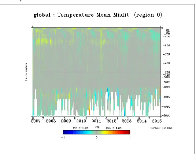
Figure 1: Average temperature misfit in K (observation – forecast) from data assimilation statistics over time and depth for the whole hindcast run (2007-2015).

The V2.3 GLO HR system experiences a slight warm bias (negative observation – forecast difference) in subsurface (25-500m) on global average as shown by Figure 1. This bias seems stronger during the last years 2013-2015. The average bias maps of 2015 ( Figure 2) show that as in V2 (not shown) part of this signal comes from the strong interannual ENSO signals in the Tropical Pacific where the near surface bias is also warm, as well as in the ACC and Gulfstream. Seasonal cold surface biases appear in the mid latitudes, linked with a lack of stratification during summer. Summer warming is injected too deep and results in subsurface spurious warming and too shallow mixed layer. Although these biases stay small (compensate) on global average, the temperature biases are slightly stronger in the V2.3 system than in the V2 system, which explains also higher RMS errors on average in the V2.3 system (Table 1).

(20)

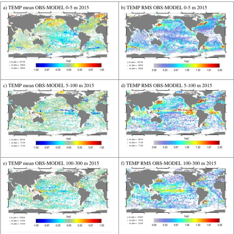
a) TEMP mean OBS-MODEL 0-5 m 2015 b) TEMP RMS OBS-MODEL 0-5 m 2015

c) TEMP mean OBS-MODEL 5-100 m 2015 d) TEMP RMS OBS-MODEL 5-100 m 2015

e) TEMP mean OBS-MODEL 100-300 m 2015 f) TEMP RMS OBS-MODEL 100-300 m 2015

Figure 2: mean (a,c, and e) and RMS (b,d, and f) observation-analysis temperature (K) differences over the calibration year 2015, averaged in the 0-5 m (a and b) 5-100m (c and d) and 100-300m (e and f) layers.

Differences are computed at the observations’ time and location. For each pixel statistics are computed in 2°x2° bins, and the size of the pixel is proportional to the number of observations falling into the bin.

3D T (K)

Mean misfit RMS misfit Mean misfit RMS misfit

(21)

V2 V2.3 V2 V2.3 V2 V2.3 V2 V2.3

0-5m -0.02 -0.03 0.57 0.65 tbc tbc tbc tbc

5-100m -0.01 -0.05 0.86 0.89 tbc tbc tbc tbc

100-300m -0.05 -0.06 0.73 0.78 tbc tbc tbc tbc

300-800m -0.02 -0.03 0.41 0.43 tbc tbc tbc tbc

800-2000m 0.00 0.00 0.15 0.17 tbc tbc tbc tbc

2000-5000m -0.03 0.02 0.14 0.22 tbc tbc tbc tbc

0-5000m -0.01 -0.01 0.38 0.41 tbc tbc tbc tbc

Table 8: GLO RMS and average temperature misfits in K (observation-model) with respect to the CORIOLIS in situ observations, in contiguous layers from 0 to 5000m, for the calibration year 2015.

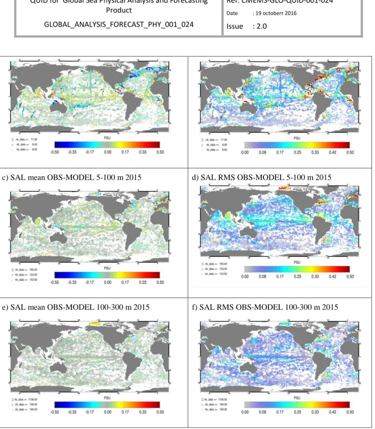
III.1.2 Salinity

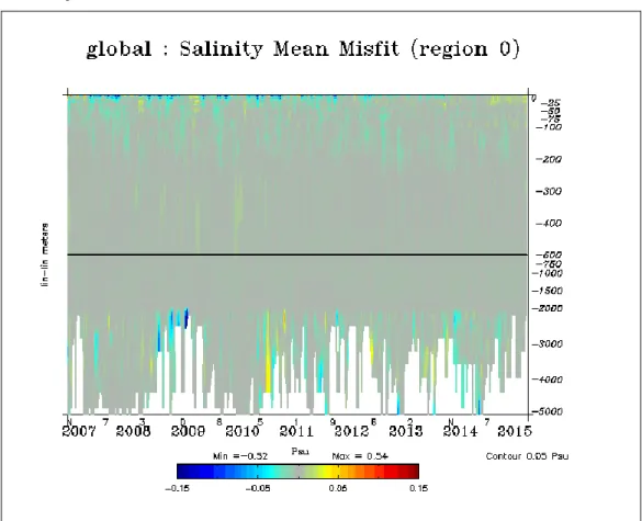
Figure 3: Average salinity misfit in psu (observation – forecast) from data assimilation statistics over time and depth, for the whole hindcast run (2007-2015).

a) SAL mean OBS-MODEL 0-5 m 2015 b) SAL RMS OBS-MODEL 0-5 m 2015

(22)

c) SAL mean OBS-MODEL 5-100 m 2015 d) SAL RMS OBS-MODEL 5-100 m 2015

e) SAL mean OBS-MODEL 100-300 m 2015 f) SAL RMS OBS-MODEL 100-300 m 2015

Figure 4: mean (a, c, and e) and RMS (b, d, and f) observation-analysis salinity (psu) residual differences over the calibration year 2015, averaged in the 0-5 m (a and b) 5-100m (c and d) and 100-300m (e and f) layers.

Differences are computed at the observations’ time and location. For each pixel statistics are computed in 2°x2° bins, and the size of the pixel is proportional to the number of observations falling into the bin.

As can be seen in Figure 3 and Figure 4 the salinity biases are very small in the V2.3, and salinity errors (mean and RMS) have been reduced from V2 to V2.3 as shown by Table 9 . A strong surface bias (GLO HR is too salty) is observed in the North Atlantic in 2015. A fresh bias due to excess precipitations is still present in V2.3 in the tropical band (Figure 4a) but has been strongly reduced with respect to V2

(23)

(not shown). In subsurface, near 100m depth, the RMS errors in the Tropical Pacific may be increased in 2015 due to the El Nino event. Fresh biases are observed in the Arctic in the 100-300m layer.

3DS(PSU)

V2 V2.3 V2 V2.3 V2 V2.3 V2 V2.3

0-5m 0.019 0.005 0.266 0.199 tbc tbc tbc tbc

5-100m 0.000 0.005 0.207 0.166 tbc tbc tbc tbc

100-300m -0.006 -0.002 0.118 0.107 tbc tbc tbc tbc

300-800m 0.000 0.000 0.055 0.057 tbc tbc tbc tbc

800-2000m 0.001 0.001 0.024 0.026 tbc tbc tbc tbc

2000-5000m -0.001 -0.003 0.013 0.017 tbc tbc tbc tbc

0-5000m 0.000 0.000 0.068 0.061 tbc tbc tbc tbc

Table 9: GLO RMS and average salinity misfits in psu (observation-model) with respect to the CORIOLIS in situ observations, in contiguous layers from 0 to 5000m, for the calibration year 2015.

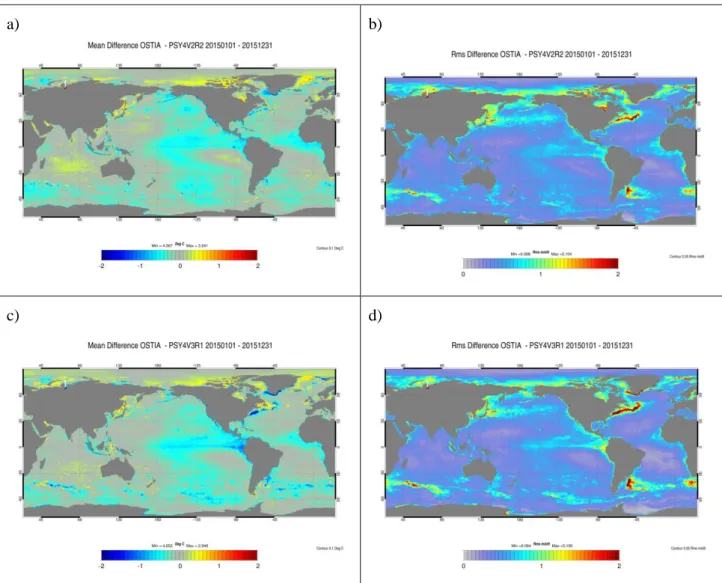
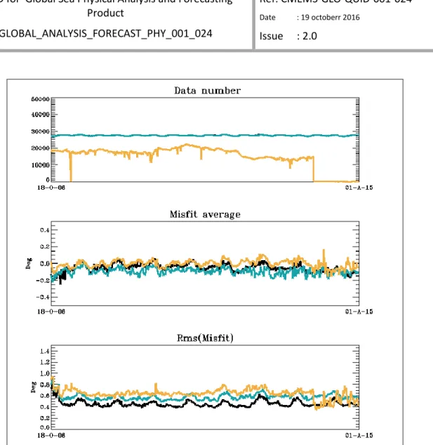
III.1.3 SST

OSTIA products are now assimilated in the GLO_HR system, as can be seen in the RMS errors of Figure 6. Some large scale biases with respect to OSTIA are reduced in V2.3 with respect to V2 (cold biases in the Indian, Eastern South Pacific, and western North Pacific). On the other hand, warm biases get stronger in V2.3, especially in regions of strong interannual warm signals such as the Eastern Tropical Pacific where El Nino took place in 2015, but also in the ACC, the Gulf Stream and the Greenland Current, resulting in a warm bias in global average of around 0.1 K, as shown in Table 1. The surface error patterns are consistent with the near surface temperature biases of Figure 2. The cold near surface bias in the mid latitudes is not diagnosed in SST, suggesting that OSTIA might be colder than in situ observations in these regions. Figure 6 suggests that OSTIA, as NOAA AVHRR, are colder than the in situ near surface observations on global average, especially at the end of the period. Figure 6 also shows seasonal fluctuations of the SST biases on global average as the lack of stratification in the model causes stronger mid latitude cold biases during (boreal) summer. The drop in the number of in situ surface data at the end of the period is due to the use of NRT observations, where most of the surface observations do not have sufficient quality flag.

NB: Regional EAN for SST could not be computed here and will be added to the next version of this document.

(24)

a) b)

c) d)

Figure 5: Mean (a and c) and RMS (b and d) residual SST errors (K) OSTIA – GLO_HR V2 (a and b) and OSTIA – GLO_HR V2.3 (c and d), computed for the calibration year 2015.

(25)

Figure 6 : The number of OSTIA (black line, assimilated data), NOAA AVHRR (blue line, independent data) and in-situ (orange line, independent data) SST observations is shown in the top panel. SST (°C) global misfits average (middle) and rms (bottom) for assimilated OSTIA SST observations (black line) and NOAA AVHRR observations (blue line), and in situ observations (orange line), for the whole hindcast run (October 2006- august 2015).

SST (K) Hindcast Forecast

V2 V2 V2 V2.3 V2 V2.3 V2 V2.3

GLO -0.01 -0.1 0.5 0.45 tbc tbc Tbc tbc

Table 10: GLO RMS and average SST misfits in K (observation-model) with respect to assimilated observations (NOAA AVHRR for V2, and OSTIA for V2.3).

(26)

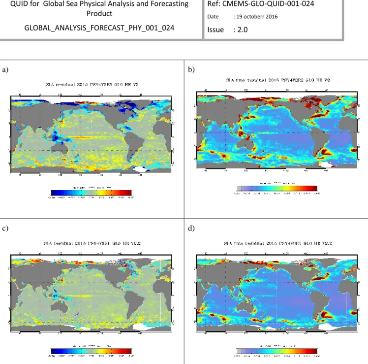
a) b)

c) d)

Figure 7: Mean residual (observation – analysis) error of SLA (m) in GLO_HR V2 (a) and V2.3 (c), and RMS residual error of SLA (m) in GLO_HR V2 (b) and V2.3 (d)

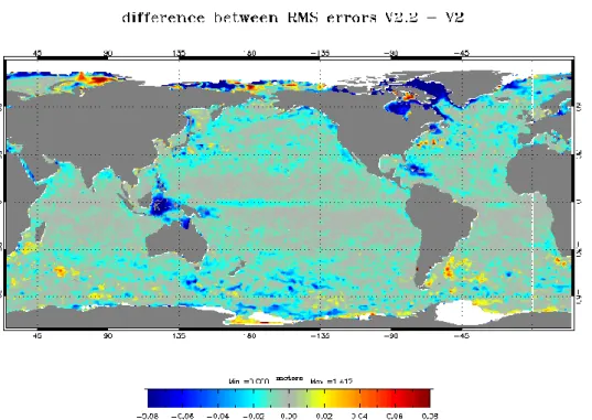
As shown in Figure 7, the SLA mean and RMS errors have been considerably reduced in the V2.3 system with respect to the previous V2 system, in nearly all regions of the ocean. This is mainly due to the use of the Desroziers criterion to adapt the observations errors online, which yield to more information from the observations being used, especially in the near coastal regions (not shown).

However, some patches of RMS errors increases can be detected in the ACC, Zapiola eddy and inside the Gulf Stream and Agulhas currents (Figure 8).

(27)

Figure 8: Difference between RMS residual (observation – analysis) errors of SLA (m) in GLO_HR V2.3 and V2. Negative values indicate that the RMS of residual errors of SLA are weaker in GLO_HR

V2.3. than in v2.

(28)

Figure 9: SLA (cm) data assimilation statistics for the HR global system with respect to along track observations (green: geosat2 and then cryosat2, blue: jason1, jason1 new orbit, Jason1 geodetic and then Altika, orange: envisat, Envisat new orbit, and then HY2, black: jason2), for the whole hindcast run (2007-2015).

The stability over time of the accuracy in terms of SLA is illustrated in Figure 9 . The RMS error is 6 cm on average over the 2007-2015 period and the average misfit oscillates between positive and negative values resulting in a small 0.63 cm bias in Table 11. The SLA bias is 0.3 cm higher in V2.3 than in V2, but the RMS misfit has improved from 6.3 cm to 5.5 cmV2.3, suggesting that the SSH variability is closer to SLA observations in V2.3 than in V2.

Seal Level Anomaly

(cm)

Mean misfit RMS of misfit Mean misfit RMS misfit

V2 V2.3 V2 V2.3 V2 V2.3 V2 V2.3

GLO 0.35 0.63 6.30 5.50 tbc tbc Tbc tbc

Table 11: GLO RMS and average SLA misfits in cm (observation-model) with respect to altimetric observations.

III.1.5 Sea Ice

Sea ice concentrations from OSI TAC are assimilated in GLO_HR V2.3, which was not the case in V2 where no sea ice concentration data assimilation was performed. This data assimilation consistently reduces the mean and RMS errors of GLO_HR V2.3 in Sea Ice Concentrations with respect to V2, as illustrated by Figure 10.

(29)

Figure 10: (observation-forecast) RMS differences of Sea ice Concentration (SIC, 0 means no ice, 1 means 100% ice cover) in the Arctic. Dark blue is the RMS error of GLO_HR with respect to assimilated OSI TAC’s SIC, light blue is the RMS of GLO_HR with respect to CERSAT SIC independent observations. Dark red is the RMS error of GLO_HR twin experiment with no sea ice concentration data assimilation (free run, as in GLO HR V2) with respect to OSI TAC’s observations, and light red is the same but with respect to CERSAT sea ice concentrations. The number of OSI TAC’s SIC data is shown in grey (units on the right y-axis).

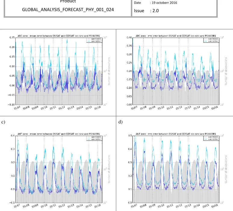
As shown by Figure 11, the GLO_HR system sees slightly too much ice during the beginning of the melting season in summer (up to 3% overestimation on average in both Arctic and Antarctic basins), while the mean error is stronger on average during winter (10 to 20% underestimation, depending on the year).

a) b)

(30)

c) d)

Figure 11: (observation-forecast) mean (a and c) and RMS (b and d) differences of Sea ice Concentration SIC (0 means no ice, 1 means 100% ice cover) in the Arctic Ocean (a and b) and

Antarctic Ocean (c and d). Dark blue is the mean or RMS error of GLO_HR with respect to assimilated OSI TAC’s SIC, light blue is the mean or RMS of GLO_HR with respect to CERSAT SIC

Observations.

Sea Ice Cover

(%)

V2 V2.3 V2 V2.3 V2 V2.3 V2 V2.3

ARC -20% 10% 30% 20% tbc tbc Tbc tbc

ACC -30% 5% 40% 25% tbc tbc Tbc tbc

Table 12: GLO_HR V2.3 RMS and average Sea Ice Concentration (observation-model) with respect to OSI TAC observations.

(31)

RMS errors are also larger during the melt season in summer (up to 20% in the Arctic and 30% in the Antarctic with respect to OSI TAC’s observations), and drop to less than 10% in winter. These RMS errors quantify the capacity of the system to capture weekly time changes in the ice cover.

In the Arctic, the error peaks without data assimilation happen at the sea ice cover minimum in September, while with data assimilation it is now during summer (July-August), while the Sea Ice is melting. This may be linked to the fact that the weekly assimilation of sea ice concentration is not fitted to constrain rapid changes in the sea ice cover in the marginal seas.

III.1.6 Surface currents

Near surface currents (near 15m depth) can be compared with velocities deduced from drifters (CMEMS) and ARGO floats (YoMaHa) trajectories (see Lellouche et al, 2013). We use these Eulerian comparisons to give an estimate of the surface currents errors, and quantify the improvement between V2 and V2.3.

The velocities have been slightly improved from V2 and V2.3 in terms of velocity values (2 and 3) as well as in terms of current directions (angle between observed and modelled velocities) (Figure 14).

a) b)

Figure 12: zonal average velocity biases (m/s) in the GLO_HR V2 (a) and GLO_HR V2.3 (b) with respect to drifters’ velocities and ARGO floats velocities, over the calibration year 2015.

The location of the main currents is very well represented, as well as their variability, but large biases persist in the western tropical Pacific (very strong in 2015 because of the El Nino event) as can be seen in Figure 15, with a spurious extension of the northern branch of the South Equatorial Current.

The currents magnitude is usually underestimated at mid-latitudes and overestimated in the tropics.

Relative errors range from 20% to 100% locally (not shown).

EAN from these metrics will be produced for CMEMS V3.

(32)

a) b)

Figure 13: scatter diagrams for GLO_HR V2 (a) and GLO_HR V2.3 (b) velocities near 15 m depth with respect to drifters’ velocities and ARGO floats velocities, for the calibration year 2015.

Figure 14: zonal average trigonometric angle (°) between the GLO_HR V2 (a) and GLO_HR V2.3 (b) velocity vectors and the drifters’ velocities and ARGO floats velocities, over the calibration year

(33)

2015. Current velocities higher than 0.1 m/s are shown in grey and velocities higher than 0.3 m/s in black.

a) observed U b) observed V

c) modeled U d) modeled V

e) f)

(34)

velocity bias (m/s) and f) meridional velocity bias (m/s) deduced from the differences between GLO_HR V2.3 and the observations.

III.1.7 Mixed Layer Depth

Large scale mixed layer depth features are captured by the GLO_HR system, as shown by Figure 16.

We note the strong interannual signal taking place in the North Atlantic in 2013-2015, where a strong cold anomaly is observed.

Figure 16 : climatological annual mean mixed layer depth (m). De Boyer Montegut climatology data (left) and GLO_HR-V2 (middle) (2013-2015 average) and GLO_HR V2.3 (right) (2013-2015 average).

Figure 17 : 2015 distributions, for the global ocean, of Mixed Layer Depth, calculated from profiles with the density criteria (MLD defined as the depth at which density difference from the surface

reaches 0.02 kg/m³) (left) and temperature criteria (MLD defined as the depth at which temperature difference from the surface reaches 0.2°C)(right); V2 is in grey, V2.3 is in blue and the

in situ observations in red.

(35)

Comparing the distributions of mixed layer depth at global scale in 2015 in Figure 17, we note that the density and temperature criteria give very different distributions, and that GLO_HR V2.3 is closer to observations than GLO_HR V2. In both V2 and V2.3, the mixed layer is too often shallower than in the observations.

EAN for this metric will be produced for V3.

III.1.8 Validation of high frequencies at tide-gauges

The GLO_HR system produces hourly outputs at the surface that can be compared with tide gauges measurements, from which we filter out the inverse barometer effect and the tides.

III.1.8.1 Sea surface Height

a) b)

Figure 18 : Taylor diagram of the sea surface height errors (2015). Comparison between observations at tide gauges and GLO_HR systems. (a): GLO_HR V2. (b): GLO_HR V2.3.

a) b)

(36)

Figure 19 : comparison of the RMS difference (a) and the correlation (b) of the sea surface height between the observations at tide gauges and the V2.3 and v2 GLO_HR systems (2015). When the RMS difference (correlation) of GLO_HR V2.3 is lower (higher) than for GLO_HR v2, the color is red,

otherwise it is yellow.

GLO_HR high frequency SSH (without tides or inverse barometer) compares well with tide gauges in many places, with a slight improvement in V2.3 with respect to V2, as shown by Figure 18, Figure 19 and Table 13.

Seal surface

height (cm)

correlation RMS of misfit Mean misfit RMS misfit

V2 V2.3 V2 V2.3 V2 V2.3 V2 V2.3

GLO 0.81 0.83 4.9 4.6 tbc tbc Tbc tbc

Table 13: averaged values of RMS difference and correlation of the sea surface height in 2015

Figure 20 : Sea surface height RMS difference (cm) between observations at tide gauges and GLO_HR V2.3 for the year 2015.

The best agreement between GLO_HR and tide gauges is found in the tropical band, as can be seen in Figure 20, while shelf regions and closed seas are less accurate.

III.2 North Atlantic: NAT III.2.1 Temperature

3D temperature accuracy results are synthesized in Table 14.

(37)

- Small biases (< 0.5K), reduced in subsurface from V2 to V2.3.

- RMS errors are large near the thermocline where the variability is higher. RMS is reduced in subsurface from V2 to V2.3.

- The modelled ocean surface is slightly too cold on average.

- The sub-surface ocean is generally warmer than the observations.

- Warm biases are found in the 2000-5000m layer but the statistics are not robust in this layer because of the fewer number of data.

3DT (K) Hindcast Forecast day 3

V2 V2.3 V2 V2.3 V2 V2.3 V2 V2.3

0-5m 0.01 0.04 0.91 1.01 tbc tbc tbc tbc

5-100m -0.09 -0.07 1.20 1.13 tbc tbc tbc tbc

100-300m -0.10 -0.06 0.92 0.88 tbc tbc tbc tbc

300-800m -0.05 -0.04 0.71 0.68 tbc tbc tbc tbc

800-2000m -0.02 -0.03 0.31 0.32 tbc tbc tbc tbc

2000-5000m -0.19 -0.10 0.33 0.28 tbc tbc tbc tbc

0-5000m -0.04 -0.04 0.60 0.58 tbc tbc tbc tbc

Table 14: NAT RMS and average temperature misfits in K (observation-model) with respect to the CORIOLIS in situ observations, in contiguous layers from 0 to 5000m.

3D salinity results are synthesized in Table 15.

- Small biases (< 0.1 psu).

- Salty bias at the surface.

- Mean error and RMS are significantly reduced in the 0-300m layer between V2 and V2.3.

3DS(PSU) Hindcast Forecast day 3

V2 V2.3 V2 V2.3 V2 V2.3 V2 V2.3

0-5m -0.083 -0.039 0.389 0.250 tbc tbc tbc tbc

5-100m -0.035 0.003 0.304 0.202 tbc tbc tbc tbc

100-300m -0.010 -0.009 0.204 0.148 tbc tbc tbc tbc

300-800m -0.004 0.000 0.101 0.095 tbc tbc tbc tbc

800-2000m 0.000 -0.003 0.049 0.049 tbc tbc tbc tbc

(38)

Table 15: NAT RMS and average salinity misfits in psu (observation-model) with respect to the CORIOLIS in situ observations, in contiguous layers from 0 to 5000m.

III.2.3 SLA

Figure 21: NAT RMS and average SLA misfits in cm (observation-model) with respect to all available altimetric missions in 2015 (black: Jason 2, cyan: SARAL/Altika, blue: HY-2, orange: Cryosat 2).

On average over the NAT zone (Table 16) we note a small positive observation – model anomaly of around 0.2 cm consistent with a cold bias. The RMS error is reduced of 1 cm on average from the previous version of the system to this new version.

(cm)

(39)

NAT -0.55 0.23 7.35 6.31 tbc tbc tbc tbc Table 16: NAT RMS and average SLA misfits in cm (observation-model) with respect to Jason 2, Saral/Altika and Cryosat2 observations. Statistics from the calibration period (year 2015) were used to build these regional estimates.

The stability over time of the GLO_HR system SLA statistics is illustrated inFigure 21, as well as the integration of all available observations (Jason 2, SARAL/Altika, HY-2, Cryosat 2).

III.3 Tropical Atlantic: TAT

III.3.1 Temperature

- Warm biases are detected in subsurface 0-800m layer.

- The warm surface bias is reduced from V2 to V2.3.

- RMS errors are large near the thermocline where the variability is higher, with a very slight increase from V2 to V2.3.

V2 V2.3 V2 V2.3 V2 V2.3 V2 V2.3

0-5m -0.10 -0.05 0.36 0.40 tbc tbc tbc tbc

5-100m -0.16 -0.19 1.01 1.10 tbc tbc tbc tbc

100-300m -0.11 -0.11 0.73 0.73 tbc tbc tbc tbc

300-800m -0.06 -0.06 0.50 0.51 tbc tbc tbc tbc

800-2000m 0.00 0.01 0.09 0.12 tbc tbc tbc tbc

2000-5000m -0.06 -0.02 0.11 0.11 tbc tbc tbc tbc

0-5000m -0.03 -0.03 0.42 0.43 tbc tbc tbc tbc

Table 17: TAT RMS and average temperature misfits in psu (observation-model) with respect to the CORIOLIS in situ observations, in contiguous layers from 0 to 5000m.

- The fresh bias at the surface in the V2 system is four times smaller in V2.3 (now <0.03 psu on average over the basin).

(40)

V2 V2.3 V2 V2.3 V2 V2.3 V2 V2.3

0-5m 0.119 0.029 0.403 0.229 tbc tbc tbc tbc

5-100m 0.030 0.015 0.223 0.170 tbc tbc tbc tbc

100-300m -0.016 -0.012 0.117 0.114 tbc tbc tbc tbc

300-800m -0.004 -0.004 0.043 0.051 tbc tbc tbc tbc

800-2000m 0.006 0.002 0.021 0.023 tbc tbc tbc tbc

2000-5000m 0.001 0.000 0.013 0.021 tbc tbc tbc tbc

0-5000m 0.003 0.000 0.068 0.061 tbc tbc tbc tbc

Table 18: TAT RMS and average salinity misfits in psu (observation-model) with respect to the CORIOLIS in situ observations, in contiguous layers from 0 to 5000m.

III.3.3 SLA

V2.3 version reduces the RMS error by 0.5 cm with respect to V2, while the bias is slightly higher (0.04 cm) and is consistent with a fresh bias.

(41)

Figure 22: TAT RMS and average SLA misfits in cm (observation-model) with respect to all available altimetric missions in 2015 (black: Jason 2, cyan: SARAL/Altika, blue: HY-2, orange: Cryosat 2).

(cm)

V2 V2.3 V2 V2.3 V2 V2.3 V2 V2.3

TAT 0.45 0.49 4.03 3.41 tbc tbc Tbc tbc

Table 19: TAT RMS and average SLA misfits in cm (observation-model) with respect to all available observations. Statistics from calibration period on year 2015 are used to build these regional estimates.

The stability over time of the GLO system SLA statistics in the TAT region is illustrated in Figure 22 as well as the integration of all available observations (Jason 2, SARAL/Altika, HY-2, Cryosat 2).

(42)

III.4 Mediterranean Sea: MED

- The bias is cold at the surface (0.1K) and warm in subsurface layers below 100m (<0.05K).

- RMS errors are slightly higher in V2.3 at the surface.

- RMS errors are larger in the 2000-5000m layer in V2.3, but results are not robust in this layer where very few observations are available, further monitoring of these errors is necessary.

V2 V2.3 V2 V2.3 V2 V2.3 V2 V2.3

0-5m 0.05 0.11 0.65 0.79 tbc tbc tbc tbc

5-100m -0.04 -0.07 0.80 0.80 tbc tbc tbc tbc

100-300m -0.02 -0.04 0.30 0.30 tbc tbc tbc tbc

300-800m 0.04 0.00 0.18 0.17 tbc tbc tbc tbc

800-2000m -0.01 -0.01 0.09 0.08 tbc tbc tbc tbc

2000-5000m 0.05 0.09 0.09 0.57 tbc tbc tbc tbc

0-5000m 0.00 -0.01 0.26 0.26 tbc tbc tbc tbc

Table 20: MED RMS and average temperature misfits in K (observation-model) with respect to the CORIOLIS in situ observations, in contiguous layers from 0 to 5000m.

- Small biases (< 0.05 psu).

- V2.3 biases smaller than V2 in the 0-100m layer but higher in the 100-800m layer.

- Surface RMS error decreases of ~ 0.15 psu over the domain in V2.3 with respect to V2.

V2 V2.3 V2 V2.3 V2 V2.3 V2 V2.3

0-5m 0.084 -0.009 0.393 0.258 Tbc tbc tbc tbc

5-100m 0.074 0.030 0.273 0.199 Tbc tbc tbc tbc

100-300m 0.003 -0.003 0.112 0.102 Tbc tbc tbc tbc

300-800m 0.003 0.005 0.044 0.044 Tbc tbc tbc tbc

(43)

800-2000m -0.004 -0.003 0.029 0.029 Tbc tbc tbc tbc 2000-

5000m 0.000 -0.025 0.016 0.044

Tbc tbc tbc tbc

0-5000m 0.004 0.002 0.087 0.071 Tbc tbc tbc tbc

Table 21 : MED RMS and average salinity misfits in PSU (observation-model) with respect to the CORIOLIS in situ observations, in contiguous layers from 0 to 5000m.

III.4.3 SLA

Figure 23: MED RMS and average SLA misfits in cm (observation-model) with respect to all available altimetric missions in 2015 (black: Jason 2, cyan: SARAL/Altika, blue: HY-2, orange:

Cryosat 2).

(44)

MED 2.26 2.50 8.59 6.10 tbc tbc tbc tbc Table 22: MED RMS and average SLA misfits in cm (observation-model) with respect to all available observations. Statistics from calibration period on year 2015 are used to build these regional estimates.

The SLA bias is more important in the MED region than in the Atlantic, and stays below 3 cm on average (Figure 23). This high value is due to strong biases of more than 3 cm in the Ionian Sea and Sicily regions (not shown). These regions are shallow and close to the coast. As a consequence, the SLA observation error is high in these zones in GLO_HR. Thus, these regions are poorly constrained and biases are observed.

III.5 South Atlantic: SAT

- Warm biases are found from the surface to 800m (~0.1K).

- RMS errors are large near the thermocline where the variability is higher.

- Mean and RMS errors slightly increase from V2 to V2.3.

V2 V2.3 V2 V2.3 V2 V2.3 V2 V2.3

0-5m -0.07 -0.09 0.54 0.62 tbc tbc tbc tbc

5-100m -0.09 -0.14 0.87 0.92 tbc tbc tbc tbc

100-300m -0.10 -0.14 0.77 0.75 tbc tbc tbc tbc

300-800m -0.04 -0.06 0.46 0.48 tbc tbc tbc tbc

800-2000m 0.01 0.01 0.15 0.15 tbc tbc tbc tbc

2000-5000m -0.03 0.04 0.12 0.20 tbc tbc tbc tbc

0-5000m -0.02 -0.03 0.40 0.41 tbc tbc tbc tbc

Table 23: SAT RMS and average temperature misfits in K (observation-model) with respect to the CORIOLIS in situ observations, in contiguous layers from 0 to 5000m.

- Small biases (< 0.01PSU) reduced from V2 to V2.3.

- Small rms error (<0.2 PSU) reduced from V2 to V2.3.