Asymmetric Time Aggregation and its Potential Benefits for Forecasting Annual Data

IHS Economics Series Working Paper 252

July 2010

Asymmetric Time Aggregation and its Potential Benefits for Forecasting Annual Data

Robert M. Kunst

Impressum Author(s):

Robert M. Kunst, Philip Hans Franses Title:

Asymmetric Time Aggregation and its Potential Benefits for Forecasting Annual Data ISSN: Unspecified

2010 Institut für Höhere Studien - Institute for Advanced Studies (IHS) Josefstädter Straße 39, A-1080 Wien

E-Mail: o ce@ihs.ac.atffi Web: ww w .ihs.ac. a t

All IHS Working Papers are available online: http://irihs. ihs. ac.at/view/ihs_series/

This paper is available for download without charge at:

https://irihs.ihs.ac.at/id/eprint/2000/

Asymmetric Time Aggregation and its Potential Benefits for Forecasting Annual Data

252

Reihe Ökonomie

Economics Series

252 Reihe Ökonomie Economics Series

Asymmetric Time Aggregation and its Potential Benefits for Forecasting Annual Data

Robert M. Kunst, Philip Hans Franses July 2010

Institut für Höhere Studien (IHS), Wien

Contact:

Robert M. Kunst

Department of Economics and Finance Institute for Advanced Studies Stumpergasse 56

1060 Vienna, Austria

: +43/1/599 91-255 email: kunst@ihs.ac.at and

Department of Economics University of Vienna Philip Hans Franses

Erasmus School of Economics Econometrics

Erasmus University Rotterdam 3000 DR Rotterdam, The Netherlands email: franses@ese.eur.nl

Founded in 1963 by two prominent Austrians living in exile – the sociologist Paul F. Lazarsfeld and the economist Oskar Morgenstern – with the financial support from the Ford Foundation, the Austrian Federal Ministry of Education and the City of Vienna, the Institute for Advanced Studies (IHS) is the first institution for postgraduate education and research in economics and the social sciences in Austria. The Economics Series presents research done at the Department of Economics and Finance and aims to share “work in progress” in a timely way before formal publication. As usual, authors bear full responsibility for the content of their contributions.

Das Institut für Höhere Studien (IHS) wurde im Jahr 1963 von zwei prominenten Exilösterreichern – dem Soziologen Paul F. Lazarsfeld und dem Ökonomen Oskar Morgenstern – mit Hilfe der Ford- Stiftung, des Österreichischen Bundesministeriums für Unterricht und der Stadt Wien gegründet und ist somit die erste nachuniversitäre Lehr- und Forschungsstätte für die Sozial- und Wirtschafts- wissenschaften in Österreich. Die Reihe Ökonomie bietet Einblick in die Forschungsarbeit der Abteilung für Ökonomie und Finanzwirtschaft und verfolgt das Ziel, abteilungsinterne Diskussionsbeiträge einer breiteren fachinternen Öffentlichkeit zugänglich zu machen. Die inhaltliche Verantwortung für die veröffentlichten Beiträge liegt bei den Autoren und Autorinnen.

Abstract

For many economic time-series variables that are observed regularly and frequently, for example weekly, the underlying activity is not distributed uniformly across the year. For the aim of predicting annual data, one may consider temporal aggregation into larger subannual units based on an activity time scale instead of calendar time. Such a scheme may strike a balance between annual modelling (which processes little information) and modelling at the finest available frequency (which may lead to an excessive parameter dimension), and it may also outperform modelling calendar time units (with some months or quarters containing more information than others). We suggest an algorithm that performs an approximate inversion of the inherent seasonal time deformation. We illustrate the procedure using weekly data for temporary staffing services.

Keywords

Seasonality, time deformation, prediction, time series

JEL Classification

C22, C53

Contents

1 Introduction 1

2 Some role-model examples 3 3 Time deformation 6 4 The algorithm 8 5 Monte Carlo evidence 12

5.1 Months and quarters ... 14 5.2 Weeks and quarters ... 17

6 An empirical application 21 7 Summary and conclusion 24

References 25 Appendix 26

1 Introduction

We are interested in predicting time-series variables that are avail- able at a subannual frequency. For example, this frequency—in the following called the ‘fine’ frequency—could be weeks. The objective is to predict the annual values, and we generally as- sume that the variable is a flow, such that the annual value is the cumulated sum of all weekly values for that year. If the variable is a stock, this does not change the main arguments, as long as the average over all weeks is in focus, as that annual value is just a multiple of the sum. In fact, the empirical example that we present here corresponds to such a stock case.

Obvious suggestions are to forecast the annual variable on the basis of an annual model or of a model tuned to the fine frequency. It is well known that prediction based on the suban- nual data and on subsequent time aggregation of the multi-step predictions is not always optimal (see, e.g., Man, 2004). Small samples and limited degrees of freedom can entail very inefficient forecasts based on models for the fine frequency. Thus, another alternative could be a partial time aggregation to a ‘crude’ sub- annual frequency and to consider time-series modelling on that frequency. In the example of weekly data availability, the crude frequency could be months or quarters.

Quite often, however, economic activity is concentrated in spe- cific parts of the year. For example, tourism in a holiday resort may be low in November and booming around Christmas and in summer. Then, much information will be contained in the third and fourth quarters and little information in the second quarter.

A forecaster may consider forming pseudo-quarters, aggregating the first four months into one observation instead of the first three. This is what will be called regrouping in the following.

We consider an algorithm that aims at spreading the seasonal variation approximately uniformly across the crude frequency.

We investigate cases where forecasts based on such an artificial crude data outperform those based on natural splits and some- times even those based on the fine frequency. This procedure could be classified as a type-III aggregation procedure in the ter- minology of Jord`a and Marcellino (2004) that aggregates regularly spaced time points into irregularly spaced time points, albeit with the ultimate aim of predicting a regularly spaced se- ries. Thus, the type-III aggregation is followed by a type-II aggre- gation that aggregates irregularly spaced data to a final regularly spaced annual series.

Our generating model at the fine frequency builds on the con- cept of time deformation. Time deformation was introduced to the econometric literature by Clark (1973) whose ideas were followed extensively in finance. Stock (1987, 1988) used the concept for business cycles at a longer and slightly irregular fre- quency, inspired by the historical work byBurns and Mitchell (1946). By contrast, we use time deformation to describe seasonal behavior within a year. The economic clock is assumed to run faster in certain seasons and to slow down afterwards. The algo- rithm approximates a reversion of the underlying time deforma- tion. We demonstrate that the success of this procedure depends on the specific design.

2

We illustrate the procedure using weekly data on temporary staffing services.

The plan of this paper is as follows. Section 2 reviews some simple cases of underlying time-series generating laws and evalu- ates the properties of annual and subannual forecasting schemes for each example. Section 3 focuses on the concept of time defor- mation and introduces the time-deformation functions that will be used in the following section. Section 4 introduces our algo- rithm that targets an approximate inversion of the underlying time deformation in given data. Section 5 reports some simula- tion experiments for time-deformed data. Section 6 analyzes an empirical application. Section 7 concludes.

2 Some role-model examples

In this section, we analyze some basic seasonal generating processes and their implications with regard to the prospects of regroup- ing on prediction. These examples are traditional in the sense that they do not refer to the concept of time deformation used in subsequent sections. We convene that the subscript τ denotes the year and w denotes the season within the year w= 1, . . . , S.

Double subscripts τ, w denote season w in year τ, with the con- vention that X_τ,1 is preceded byX_τ−1,S, for example. Details on calculation are deferred to the appendix.

Example 1. Assume Z_τ = PS

w=1X_τ,w, where (X_τ,w) is a random walk such thatXτ,w =Xτ,w−1+ετ,w. (ετ,w) is independent white noise with varianceσ²_ε. Then, as shown in the appendix, the

conditional expectation forecast formed at time point (τ, S) for Zτ+1 will beSXτ,Swhen it is based on the subannual information.

The mean squared error of the subannual forecast is σ²_εPS j=1j². If only annual information is available, Zτ −Zτ−1 follows a first- order MA process. The MSE of the naive annual forecast Zτ

is σ_ε²(PS

j=1j²+PS−1

j=1 j²), which can exceed the subannual MSE substantially for larger S. The optimal annual forecast yields an only slightly smaller MSE, typically still much in excess of the subannual MSE. Now suppose we can regroup into two groups.

Then, the optimal prediction grouping will consist of PS−1 w=1Xτ,w

in the first group andXτ,S in the second group. The last season is isolated, as it contains the most recent information that is most useful for predicting the upcoming year. The forecast based on the last season only corresponds exactly to the forecast based on the full subannual information.

Example 2. AssumeX_τ,w =X_τ−1,w+ε_τ,w, a seasonal random walk, otherwise keep the design of example 1. Then, the forecast based on annual data and the forecast based on subannual data are identical, such that seasonal information has no additional value. This result is invariant to any regrouping of the seasonals.

Example 3. Assume Xτ,w = δw +ετ,w, purely deterministic seasonality. Then, the conditional expectation forecasts based on annual as well as subannual data are identically PS

w=1δw, which yields a forecast variance ofSσ_ε². Again, the result is invariant to any regrouping.

Example 4. Assume S = 4, and X_τ,w is generated by a periodic process that is a seasonal random walk for w = 1,2

4

and white noise for w = 3,4. Quarterly data entail a MSE of 4σ_ε². If only annual data are available, the MSE increases to around 5.236σ_ε², as derived in the appendix. Forecasts based on regrouping fall in between these two benchmarks. Traditional semesters, with the first semester formed from quarters 1 and 2, yield a seasonal random walk for the first semester and white noise for the second semester. The MSE is the same as in the quarterly case. Grouping the first quarter separately from the three other quarters yields a seasonal random walk for the first quarter and an ARIMA(0,1,1) for the second group formed from quarters 2–4. The resulting forecast has a variance of 5σ²_ε, closer to the inefficient annual than to the efficient quarterly.

Example 5. Modify the conditions in Example 4 such that the seasonal random walk in the first two quarters is replaced by a random walk that adds a white-noise term to the first quar- ter for the second quarter and another white-noise term to the second quarter for the first quarter of the next year. In this de- sign, the optimal forecast for the next year based on quarters just uses twice Xτ−1,2 and achieves a forecast error variance of 7σ²_ε. By contrast, for the forecast based on annual data error variance increases palpably to 10σ_ε². Here, grouping plays a role. Direct semester grouping yields an ARIMA(0,1,1) model with the im- plied forecast error of 7.84σ_ε². By contrast, splitting the year into a first quarter and the remainder yields a forecast that is difficult to evaluate analytically, due to the complex correlation structure among forecast errors. We used some Monte Carlo that indeed conformed to the analytical results for the other cases. For the

regrouped prediction, it yields an error variance well above 9σ²_ε. The intuitively beneficial regrouping entails an inefficient fore- cast that is closer to the uninformative annual than to the most informative quarterly prediction.

Clearly, the reaction to regrouping the subannual observations is quite heterogeneous across data-generating processes. While no general recommendation can be given based on these examples, it appears that strong and homoskedastic seasonality usually en- tails robustness to regrouping, while strong serial correlation with weak seasonal cycles may lead to considerable sensitivity to re- grouping. Collecting subannual observations with similar time- series dynamics can be beneficial for regrouping schemes, and seasonal heteroskedasticity can also be influential.

3 Time deformation

In a sense, the concept of time deformation is ubiquitous in ob- served economic variables. Economic activity on stock markets, for example, is low while the stock market is closed, such that it may give the impression that time is running faster while the stock exchange is operating. Similarly, heating is less needed in summer, such that the economic time of heating is running faster in winter, slowing down in spring and coming to a standstill on a hot day.

Following a seminal contribution by Clark (1973), the con- cept has been applied often to financial data with high observa- tional frequency (for example, see Ghysels et al., 1995), and

6

less often to business cycles (seeStock, 1987, 1988) or to intra- year seasonal variation (Jord`a and Marcellino, 2004). For a theoretical exposition of results on a class of time-deformation models, see also Jiang et al. (2006).

Seasonal variation, however, has the advantage that the start- ing points and ends of the intervals of concern are exogenous, at the begin and end of calendar years. By contrast, limits of busi- ness cycles are more difficult to determine, and the definition of troughs and peaks may be subject to some subjective expertise, such as the known NBER chronology.

Within the time interval of concern—in the case of seasonality, one year—a deformation function s = g(t) defines the transfor- mation of calendar time t to economic time s. Typically, the function should be invertible, continuous, and monotonic. It may be acceptable to admit violations of strict monotonicity and to allow for episodes without any economic activity.

An example of a deformation function is plotted in Figure 1.

The graph depicts the function s=t^0.2

on the unit interval. Dotted lines signal the points where one, two, and three quarters of calendar time have elapsed. The first quarter is the most active, and actually almost 80% of economic activity is located in the first three months of the year, if the unit interval is equated to a calendar year.

A comparable plot for the time deformation function s= arcsint

π/2

0.0 0.2 0.4 0.6 0.8 1.0

0.00.20.40.60.81.0

t

s

Figure 1: The deformation functiont^0.2 in [0,1].

is given as Figure 2. Economic activity is assumed to run faster toward the end of the year rather than at the beginning. Gener- ally, time deformation appears to be less radical than for Figure 1.

These two deformation functions will serve as role models for the generating processes in the simulations. It is easy to gen- eralize these functions to allow for several high-activity episodes through the year but we wish to keep the design as simple as possible.

4 The algorithm

Assume a time-series variable Xτ,w is observed at a subannual

‘fine’ frequency S1, such that observations X_τ,w are available for 8

0.0 0.2 0.4 0.6 0.8 1.0

0.00.20.40.60.81.0

t

s

Figure 2: The deformation function ^arcsin_π/2^t in [0,1].

τ = 1, . . . , T andw= 1, . . . , S1. An annual variableZτ is defined as a time aggregate:

Zτ =

S1

X

w=1

Xτ,w, τ = 1, . . . , T.

For example, S1 = 52 represents weekly availability and S1 = 12 corresponds to monthly data.

The objective is to forecast the next annual valueZT+1, i.e. to find a function of the observed values that approximates ZT+1 as closely as possible. Considered criteria for prediction accuracy are the mean squared error (MSE), the mean absolute error (MAE), and the relative ranking among rival predictors.

A traditional approach for model-based prediction is mod- elling on an annual basis:

Zτ =f(Zτ−1, Zτ−2, . . .) +ετ,

usually with a linear function f(.), and plugging in the estimated structure to approximate conditional expectations:

Zˆ_τ,I = ˆf(Z_τ−1, Z_τ−2, . . .).

This forecast will be called forecast I in the following, and we will focus on autoregressive f models with a lag order determined by information criteria.

Alternatively, modelling may rely on the S1 frequency, using xw in short for xτ,w:

xw =f(xw−1, xw−2, . . .) +εw.

In order to capture the seasonal variation in the data, thef func- tion may contain seasonal dummy variables for the S1 seasons.

In practice, with unknown parameters, this approach requires the estimation of S1 parameters on top of thep coefficients of an au- toregressive specification. Once the model has been estimated from data, forecasts at horizons 1 to S1 can be generated by it- eratively using

ˆ

xw = ˆf(xw−1, xw−2, . . .;δw),

whereδ_w denotes the seasonal dummy variables. This first yields ˆ

xT+1,1. At horizon 2, the unobserved first argument xT+1,1 is replaced by the one-step forecast, and this scheme is followed until ˆxT,S₁ is attained. Finally, time aggregation yields

Zˆ_τ,II =

S1

X

w=1

ˆ x_τ,w.

This forecast will be called forecast II in the following.

10

An intermediate approach may rely on a ‘crude’ frequency S2 that is assumed to be an integer factor of S1. For example, if S1 = 52, thenS2 = 4 orS2 = 2 are possible values. S1 = 12 would admit S2 = 2,3,4. Using S2 instead of S1 may be motivated by the promise of a simpler model structure and thus more efficient forecasts. We shall see that indeed forecasts based on slightly cruder frequencies tend to dominate those based on extremely fine frequencies.

The traditional approach is to aggregate the data at frequency S1 to the cruder frequencyS2 by keeping equidistant time points.

Then, a modelling technique analogous to forecast II results in a forecast III. This requires the estimation of S2 < S1 dummy coefficients, and the resulting gain in degrees of freedom can be used to extend the lag order of the autoregression.

Finally, the regrouping approach proceeds as follows. Like model III, it is also based on the frequencyS2. However, it starts from seasonal variance estimates

ˆ

σ²_w = 1 T −1

T

X

τ=1

(xτ,w−x¯w)², w = 1, . . . , S1.

The sum of these variance estimates ˆσ² measures the dispersion in the observed variable, although of course it is not tantamount to the straightforward sample variance. For ease of notation, we will not use hats in the following. We now aim at distributing this variation σ² uniformly across the year. This is done as follows.

The first artificial observation xτ;1 accumulates all original data points xτ,w, w = 1, . . . , K, such that

K = min{k:

k−1

X

t=1

σ_w² + 1

2σ_k² > σ² S2

.}

The observationxτ,K+1 at frequencyS1starts the second artificial observation xτ;2. This scheme is followed in analogy until all observations are regrouped, for all τ = 1, . . . , T. The forecast based on this algorithm will be called forecast IV in the following.

The intuition behind our regrouping scheme and, in particu- lar, our definition of K is simple. The basic aim is to distribute the variance contributions uniformly across the crude-frequency units. As long as the sum of the fine-frequency variance contri- butions is less than the proportional share, fine-frequency data are accumulated. When the accumulated sum of variances trans- gresses this proportional share, the marginal component is al- lotted either to the ‘old’ regrouped data point or a new one is started, depending on whether its half value is less or larger than the remaining discrepancy.

A difference in calculating forecast IV relative to forecast II and III is that no seasonal dummy constants are used in con- structing the time-series models. We experimented with adding dummy constants but this led to a deterioration of predictive accuracy in all experiments. This is also well in line with the original intention of regrouping as a crude means of reverting the time deformation in the data, which by construction should result in a non-seasonal time series.

5 Monte Carlo evidence

As Section 2 demonstrates, the reaction of forecast precision to time aggregation can be quite heterogeneous. The simulation ex-

12

periments reported in this section provide additional insight into such reaction patterns. Intuitively, a procedure that aims at re- verting time deformation should show its strongest performance with data generated by time deformation. The Monte Carlo sim- ulations show whether this intuition is well grounded.

Denoting economic time by s, we simulate the first-order au- toregressive process

Xs =φXs−1+εs,

with GaussianN(0,1) errorsε. In the basic version of the design, we setφ= 0.99, such that the process becomes strongly correlated but it is still stable.

To this process, we apply one of several time-deformation spec- ifications with different continuous and monotonic one-one func- tions g(t), [0,1]→[0,1]. The deformation function

s= 2

πarcsint, t ∈[0,1],

accumulates fast at the beginning and end of the year and in- creases more slowly in ‘summer’. The deformation function

s =t^δ, t∈[0,1],

behaves differently for δ <1 andδ >1. For large δ, it speeds up economic activity toward the end of the year, while it focuses on the beginning for δ <1. We chooseδ = 0.2 for a basic design.

In our simulations, we assume that data are generated though not observed at the calendar time represented by t. Observed data are at the ‘fine frequency’ S1. The transformation from the basic economic-time process to calendar time works as follows.

As long as t =g⁻¹(s)< S₁⁻¹, the observationsXs are aggregated into the first fine seasonal unit, those in the intervalt =g⁻¹(s)∈ (S₁⁻¹,2S₁⁻¹] into the second fine unit, and so on.

5.1 Months and quarters

All processes are generated for 5 to 15 years, with some reason- able burn-in. Then, we predict the following year by each of the outlined prediction models: the annual model, the monthly model (S1 = 12), the quarterly model (S2 = 4), and regrouped pseudo-quarters.

Figure 3 gives exemplary time plots of the two basic generat- ing processes. Fine seasonal intervals were set at S1 = 12, while the basic process was generated at 250 units per year. Thus, the design corresponds to business days in economic time and measurement in calendar months. These plots demonstrate the rather extreme patterns of seasonal variation, with activity con- centrated in specific parts of the year, while they also emphasize the irregular and non-repetitive nature of the seasonal cycle.

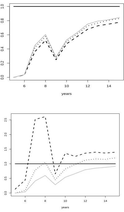
Figure 4 depicts the relative predictive accuracy, with the an- nual model used as a benchmark. As the sample size increases, simple aggregate annual data (model I) tend to yield acceptable predictions, and gains for any disaggregation become the excep- tion. For small samples, disaggregation effects can be substantial.

In the t^0.2 design, regrouping (model IV) yields similar results as the rival models II and III, while regrouping dominates defini- tively in the arc-sine design.

Related experiments are depicted in Figure 5, where model III 14

Figure 3: 16 years of generated monthly data. Deformation functions are s = t^0.2, t∈[0,1] ands= arcsin^2t_π, t∈[0,1].

6 8 10 12 14

0.00.20.40.60.81.0

years

6 8 10 12 14

0.00.51.01.52.02.5

years

Figure 4: Ratios of prediction MSE for fine seasonal frequency (dashed), crude seasonal frequency (dotted), and regrouping procedure (gray) to the annual model.

Generating process is based ont^0.2for the top graph and on arcsin^2t_π for the bottom graph.

16

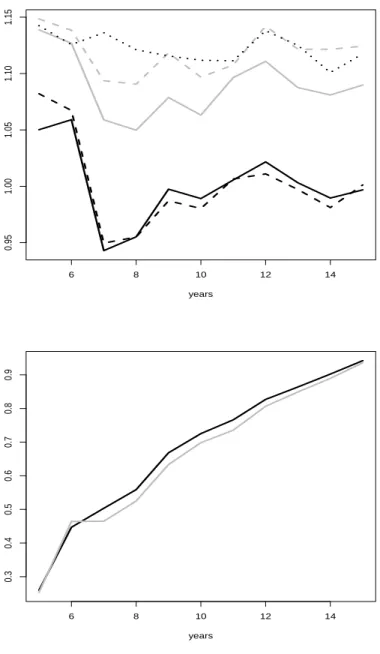
is used as a benchmark. In the left graph, the nonlinearity para- meter is allowed to vary from δ = 0.2 to δ = 0.6. Only for the designs with more extreme deformation, gains for regrouping are recognizable. In the right graph, the experiment for the arc-sine generator was repeated with AIC instead of BIC as the lag selec- tion criterion. The regrouping algorithm is substantially better than model III, and even better than the fine-seasons model II, as shown in Figure 4. The AIC version is actually better than the BIC version for most sample sizes, and it also tends to underscore the benefits of regrouping.

In summary, the simulations for the case of months and quar- ters are a bit disappointing for t^δ deformation and more sup- portive of regrouping for arc-sine deformation. This distinction matches intuition insofar as the main activity is concentrated to- ward the end of the year in the latter case, such that the most informative last month typically also becomes the last pseudo- quarter, an important cornerstone for predicting the coming year.

Conversely, in the former case the main activity in the first month has much less relevance for the next year.

5.2 Weeks and quarters

All processes are generated for 5 to 15 years, with some reason- able burn-in. Then, we predict the following year by each of the outlined prediction models: the annual model, the weekly model (S1 = 52), the quarterly model (S2 = 4), and regrouped pseudo- quarters. The frequency S1 = 52 was chosen appropriately, such that it is divisible by the quarterly frequency.

6 8 10 12 14

0.951.001.051.101.15

years

6 8 10 12 14

0.30.40.50.60.70.80.9

years

Figure 5: Ratios of prediction MSE for regrouping algorithm to the model using traditional quarters. Upper graph uses δ = 0.2 (black solid), δ = 0.3 (black dashes), δ= 0.4 (gray), δ= 0.5 (gray dashes), and δ= 0.6 (dots), with generating process based on t^δ. Lower graph uses arc-sine generating process, with black curve for BIC selection and gray curve for AIC selection.

18

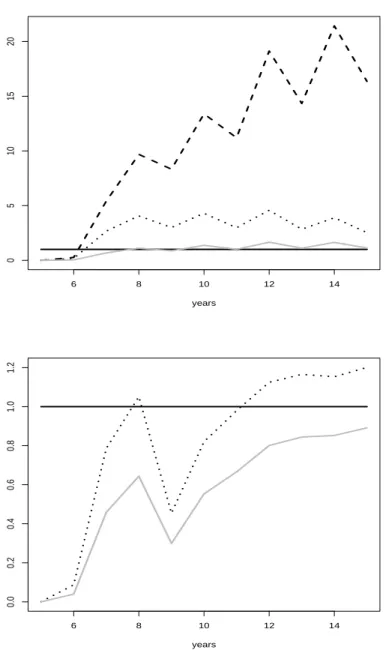
We note that the basic generating model is identical to the pre- vious subsection but the finest available frequency has changed.

Figure 6 shows that the additional information from the weekly observations is difficult to exploit. The weekly model is inferior at all sample sizes. For the arc-sine generating model, this inferi- ority is so pronounced that its MSE ratio had to be omitted from the graph. By contrast, the regrouping algorithm works well. For geometric deformation, it achieves the values set by the annual model, thus beating the forecast based on calendar quarters by a wide margin. For arc-sine deformation, regrouping is preferable to all rivals, including the annual model.

6 8 10 12 14

05101520

years

6 8 10 12 14

0.00.20.40.60.81.01.2

years

Figure 6: Ratios of prediction MSE for disaggregated prediction models to the annual model. Generating process usesδ = 0.2 in the upper plot, and the arc-sine model in the lower plot. Solid line represents the annual prediction, dashed curve is for forecast based on weeks (upper plot only), dotted curve for quarters, and gray curve for regrouped pseudo-quarters.

20

6 An empirical application

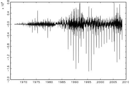
Weekly data on numbers of people who are under contract of Randstad temporary staffing services are available for the years 1967–2008, i.e. for 42 years. When years had 53 weeks, the data have been adjusted such that 52 weeks per year emerge through- out. Figure 7 displays a time-series plot of the Randstad data.

The trending impression of the data insinuates some transfor- mation, as estimated autoregressions may tend to have unstable roots, which is often detrimental for prediction. For this reason, we also considered first differences of the original data, as they are shown in Figure 8. Clearly, the extremely leptokurtic and het- eroskedastic appearance of this data suggests that its prediction could be difficult.

First, we apply the forecasting procedures as outlined above to the original data. We generate out-of-sample one-step autoregres- sive forecasts for the last 14 years of the sample, using expanding windows. Thus, the forecast for the year 2008 uses 41 years of observations, while the forecast for the year 1995 uses 28 years.

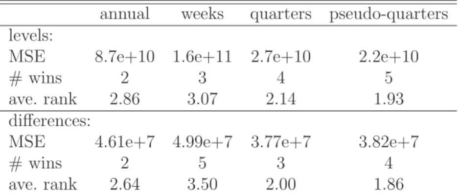
All empirical results are summarized in Table 1.

Averaging squared errors across the 14 predicted annual fore- casts yields the expected large numbers. In relative terms, the forecast based on weekly observations has an MSE that is 1.9 times as large as the annual forecast MSE, while the forecast based on quarters has an MSE that is only 0.31 the annual fore- cast MSE. According to this crude evaluation, the regrouping algorithm wins with 0.25 times the annual MSE. However, the variation across years is so sizeable that this summary measure

Figure 7: Weekly data for Randstad staffing services for the years 1967–2008.

Figure 8: First differences of the Randstad data depicted in Figure 7.

22

Table 1: Forecasting annual values 1995–2008 of the Randstad data.

annual weeks quarters pseudo-quarters levels:

MSE 8.7e+10 1.6e+11 2.7e+10 2.2e+10

# wins 2 3 4 5

ave. rank 2.86 3.07 2.14 1.93

differences:

MSE 4.61e+7 4.99e+7 3.77e+7 3.82e+7

# wins 2 5 3 4

ave. rank 2.64 3.50 2.00 1.86

Note: MSE is the average squared error across the predicted years; ‘# wins’ is the number of cases where the respective model achieves the smallest error; ‘ave. rank’

is the average rank across all 14 cases.

is unreliable. It is of more interest that the regrouping technique achieves a better accuracy than calendar quarters in 9 out of 14 years. The regrouping algorithm loses the duel in the years 2002–

2003 and 2005–2007. In 5 years, it achieves the best forecast of all four models, while it never comes in last.

Next, we apply the same prediction models to the differenced data. In a naive average MSE evaluation, calendar quarters and regrouped quarters achieve 0.81 and 0.82 of the annual average MSE. Again, performance across years is quite heterogeneous.

In a direct comparison, regrouped predictions are better than calendar quarters in 10 out of 14 cases and are best of all four models in four cases. This time, it is the earlier years that show a slight preference for traditional calendar quarters.

7 Summary and conclusion

We demonstrate that the potential benefits of ‘seasonal gerry- mandering’ in the sense of regrouping higher-frequency observa- tions into lower-frequency aggregates that conform to economic time rather than calendar time depend on the underlying data- generating process. Regular or even deterministic seasonal vari- ation yields poor prospects for such procedures, while existing seasonal time deformation may be more supportive.

In our simulation experiments, we find that seasonal regroup- ing yields good results for prediction within specific sample-size windows of less than ten years. Whereas the value of this time horizon may be sensitive to the assumed autocorrelation, the pat- tern is likely to be systematic. In large samples, fine-frequency structures can be estimated consistently and reliably, such that the finest frequency often entails the most precise prediction. In very small samples, simple models with low parameter dimen- sion typically yield the best forecasts. The window between the small-sample and the large-sample case is of interest here.

In our empirical application, we see some benefits for the re- grouping procedure, which may indicate that the sample is actu- ally within the mentioned size window. We opine that the many irregularities of the data example are typical for similar applica- tions to economics data.

24

References

[1] Burns, A.F., and Mitchell, W.C. (1949) Measuring Business Cycles. NBER, New York.

[2] Clark, P.K. (1973) ‘A Subordinated Stochastic Process Model with Finite Variance for Speculative Prices,’ Econo- metrica 41, 135–155.

[3] Ghysels, E., C. Gourieroux, and J. Jasiak (1995)

‘Trading Patterns, Time Deformation and Stochastic Volatil- ity in Foreign Exchange Markets,’ Working paper, University of Montreal.

[4] Jiang, H., Gray, H.L., and W.A. Woodward (2006)

‘Time-frequency analysis—G(λ)-stationary processes,’Com- putational Statistics & Data Analysis 51, 1997–2028.

[5] Jord`a, `O., and M. Marcellino (2004) ‘Time-scale transformations of discrete time processes,’ Journal of Time Series Analysis 25, 873–894.

[6] Man, K.S. (2004) ‘Linear prediction of temporal aggre- gates under model misspecification,’ International Journal of Forecasting 20, 659–670.

[7] Stock, J.H. (1987) ‘Measuring Business Cycle Time,’Jour- nal of Political Economy 95, 1240–1261.

[8] Stock, J.H. (1988) ‘Estimating Continuous-Time Processes Subject to Time Deformation,’Journal of the American Sta- tistical Association 83, 77–85.

[9] Working, H. (1960) ‘Note on the Correlation of First Dif- ferences of Averages in a Random Chain,’ Econometrica 28, 916–918.

Appendix

This appendix contains detailed derivations for the examples of Section 2. Most of them rely on the feature that prediction based on data at the generating frequency entails a straightforward eval- uation of variances, while first differences of annual data follow first-order moving-average processes. The minimum forecast vari- ance is then slightly smaller than the variance of the first differ- ences. The role-model case of the Lemma 1 can be used with little variation in all examples.

Lemma 1 Assume the random walk with independent increments Xτ,w = Xτ,w−1 +εt and its annual aggregate Zτ = PS

w=1Xτ,w. The forecast error variance using the annual aggregate is given as

S(S²−1)²σ²_ε 6{2S² + 1−Sp

3(S²+ 2)}, denoting σ_ε² = varεt.

Proof. With an insubstantial modification, this is the situa- tion analyzed byWorking(1960), who obtained the main result that Zτ −Zτ−1 =ητ follows a first-order moving-average process ητ =ξτ +θξτ−1 with first-order correlation

ρ1 = S²−1 2(2S²+ 1)

26

and variance

var(ητ) = S(2S²+ 1) 3 =σ²_η.

For some of our arguments, it is convenient to note that this expression follows from a triangular weighted sum of errors via

σ_η² =σ_ε²(

S

X

w=1

w²+

S−1

X

w=1

w²),

a two-sided weighted sum of error variances at the generating frequency. Solving the quadratic equation ρ1 =θ/(1 +θ²) yields

θ= 2S²+ 1−Sp

3(S²+ 2)

S² −1 .

The variance var(ξτ) = σ_ξ² corresponds to the minimum forecast variance and evolves from evaluating

σ²_ξ = σ_η² 1 +θ².

Working (1960) remarks that, for larger S, ρ1 approaches 0.25, and even the smallestS = 2 yieldsρ1 = 1/6. Also note that θ ≈ρ1, and that σ_ξ² is only slightly smaller than σ_η², the forecast variance due to the naive forecast Zτ that incorrectly assumes that it follows a random walk.

Example 1. First assume disaggregated data are available.

Then

Zˆτ+1 = E(Zτ+1|Xτ,s, . . . , Xτ,1, . . .)

= E(

S

X

w=1

Xτ+1,w|Xτ,s, . . .) =SXτ,S,

and thus

E(Zτ+1−Zˆτ+1)²

= E{SXτ,S+

S

X

w=1

(S−w+ 1)ετ+1,w−SXτ,S}²

= E{

S

X

w=1

(S−w+ 1)ετ+1,w}² =σ_ε²

S

X

w=1

w².

If only annual data are available, Lemma 1 can be applied di- rectly. From the proof of the Lemma, observe that σ²_ξ consider- ably exceeds the above expression that is a one-sided weighted sum. The correction factor is too close to one to compensate this discrepancy.

Example 2. In this case, Zτ −Zτ−1 is independent white noise at the annual frequency, and both the forecast for annual and for disaggregated data are clearly given as ˆZτ+1 =Zτ.

Example 3. Denote the information set formed by past ob- servations {Xs, s≤τ} byHτ(X). By definition,

Zτ =

S

X

w=1

(δw+ετ,w) and hence

E(Zτ+1|Hτ) =

S

X

w=1

δw.

The conditional expectation is identical if dataXτ,ware available, and hence also the concomitant prediction error variance does not change.

Example 4. First consider the annual variable. All calcula- tions closely follow the proof of Lemma 1. Here,

Zτ+1−Zτ =

4

X

w=1

ετ+1,w−

2

X

w=1

ετ,w,

28

an MA(1) process ητ = ξτ +θξτ−1 with variance 6σ_ε², first-order covariance −2σ_ε², and hence first-order correlation ρ1 = −1/3.

The implied MA coefficient follows from equating θ

1 +θ² =−1 3, which yields θ = −0.5∗(3−√

5) ≈ −0.382. The MSE is the variance of the implied white noise ξt or

σ_ξ² = 6σ_ε²/(1 +θ²)≈5.236σ²_ε.

The conditional expectation of Zτ+1 based on quarterly data is Xτ,1+Xτ,2, which yields a prediction error of just

Zτ+1−Xτ,1 +Xτ,2 =

4

X

w=1

ετ+1,w,

with variance 4σ²_ε.

Example 5. The generating process

Xτ,w =











X_τ−1,2+ε_τ,1, w = 1, Xτ,1+ετ,2, w= 2,

ε_τ,w, w= 3,4, has the forecast based on quarterly data

E(Zτ+1|Xτ,4, Xτ,3, . . .) = 2Xτ,2

with error variance

E(Zτ+1−2Xτ,2)² = E(2ετ+1,1+ετ+1,2+ετ+1,3+ετ+1,4)²

= 7σ_ε².

By contrast, if only annual data are available, Zτ −Zτ−1 = ητ

again follows a first-order MA process ητ = 2ετ,1+

4

X

w=2

ετ,w+ετ−1,2 −

4

X

w=3

ετ−1,w,

with variance σ²_η = 10σ_ε², ρ1 = −0.1, and concomitant θ ≈

−0.1010. This results in a prediction error variance of around 9.899σ_ε². The two regrouping variants can be evaluated similarly but calculations become a bit involved. As outlined in the text, they were determined by calculation and confirmed by Monte Carlo at 7.84σ²_ε for semesters and at slightly above 9σ_ε² for group- ing into the first quarter and the remaining quarters as pseudo- semesters.

30

Authors: Robert M. Kunst, Philip Hans Franses

Title: Asymmetric Time Aggregation and its Potential Benefits for Forecasting Annual Data Reihe Ökonomie / Economics Series 252

Editor: Robert M. Kunst (Econometrics)

Associate Editors: Walter Fisher (Macroeconomics), Klaus Ritzberger (Microeconomics)

ISSN: 1605-7996

© 2010 by the Department of Economics and Finance, Institute for Advanced Studies (IHS),

Stumpergasse 56, A-1060 Vienna   +43 1 59991-0  Fax +43 1 59991-555  http://www.ihs.ac.at

ISSN: 1605-7996