On the meridional ageostrophic transport in the tropical Atlantic

(1)

https://doi.org/10.5194/os-13-531-2017

On the meridional ageostrophic transport in the tropical Atlantic

Yao Fu¹, Johannes Karstensen¹, and Peter Brandt^1,2

1GEOMAR Helmholtz Centre for Ocean Research Kiel, Kiel, Germany

2Christian-Albrechts-Universität zu Kiel, Kiel, Germany Correspondence to:Yao Fu (yfu@geomar.de)

Received: 9 December 2016 – Discussion started: 9 January 2017 Revised: 8 May 2017 – Accepted: 25 May 2017 – Published: 6 July 2017

Abstract. The meridional Ekman volume, heat, and salt transport across two trans-Atlantic sections near 14.5^◦N and 11^◦S were estimated using in situ observations, wind products, and model data. A meridional ageostrophic velocity was obtained as the difference between the directly measured total velocity and the geostrophic velocity derived from observations. Interpreting the section mean ageostrophy to be the result of an Ekman balance, the meridional Ekman transport of 6.2±2.3 Sv northward at 14.5^◦N and 11.7±2.1 Sv southward at 11^◦S is estimated. The integration uses the top of the pycnocline as an approximation for the Ekman depth, which is on average about 20 m deeper than the mixed layer depth.

The Ekman transport estimated based on the velocity observations agrees well with the predictions from in situ wind stress data of 6.7±3.5 Sv at 14.5^◦N and 13.6±3.3 Sv at 11^◦S. The meridional Ekman heat and salt fluxes calculated from sea surface temperature and salinity data or from high- resolution temperature and salinity profile data differ only marginally. The errors in the Ekman heat and salt flux calculation were dominated by the uncertainty of the Ekman volume transport estimates.

1 Introduction

In the tropical Atlantic Ocean, strong and steady easterly trade winds generate a poleward meridional flow in the surface layer. According to the classical linear theory of Ekman (1905), under the momentum balance between steady wind stress and Coriolis force, the wind-driven flow spirals clock- wise with depth, the Ekman spiral, while the vertical integration of the spiral results in a net volume transport to the right of the wind direction (Northern Hemisphere), the Ek- man transport. A convergence is created in the subtropics,

where the poleward Ekman transport induced by the trade winds interacts with the equatorward Ekman transport induced by the mid-latitude westerlies. In simple linear vor- ticity theory, the Ekman convergence in subtropics drives an equatorward Sverdrup transport that explains many aspects of the wind-driven gyre circulation, such as the subtropical cells (STC). Schott et al. (2004) calculated the Ekman di- vergence (21–24 Sv, 1 Sv=10⁶m³s⁻¹) between 10^◦N and 10^◦S in the tropical Atlantic using climatological wind to infer the strength of the STC; Rabe et al. (2008) further analysed the variability of the STC using the same sections based on assimilation products, and found that on timescales longer than 5 years to decadal, the variability of poleward Ekman di- vergence leads the variability of geostrophic convergence in the thermocline.

The meridional Ekman transport is, depending on the latitude, an important upper layer contribution when estimat- ing the strength of the Meridional Overturning Circulation (MOC, Friedrichs and Hall, 1993; Klein et al., 1995; Wijffels et al., 1996). The variations in the meridional Ekman transport have been found to cause barotropic adjustment of the MOC in the ocean interior on different timescales. Cunning- ham et al. (2007) reported that the upper ocean had an im- mediate response to the changes in Ekman transport at sub- seasonal to seasonal timescales, while Kanzow et al. (2010) found that on the seasonal timescale, the Ekman transport was less important than the mid-ocean geostrophic transport, whose seasonal variation was dominated by the seasonal cycle of the wind stress curl. McCarthy et al. (2012) analysed a low MOC case during 2009 and 2010, and also pointed out that on the interannual timescale, although the Ekman transport played a role, its variability was relatively small compared to the variability in mid-ocean geostrophic transport, especially in the upper 1100 m.

(2)

Of interest for large-scale overturning studies are also the meridional Ekman-driven heat and freshwater fluxes that provide an important upper layer constraint, for example, for geostrophic end point arrays (McCarthy et al., 2015; Mc- Donagh et al., 2015). In many cases, sea surface temperature (SST) has been found to be a sufficient constraint for the Ekman layer temperature (Wijffels et al., 1994; Chere- skin et al., 2002). This probably is not too much of a surprise as the heat flux is primarily determined by the transport and less by the relatively small variability in temperature. How- ever, the unresolved vertical structure of the water column could lead to an unknown bias, for example, due to the difference between the mixed layer depth (MLD) and the depth of the Ekman layer. An extreme case has been reported for the northern Indian Ocean at 8^◦N at the end of a summer monsoon event (Chereskin et al., 2002), where the direct Ek- man temperature transport was 5 % smaller when using the temperature within the top of the pycnocline (TTP, as a proxy of the Ekman layer depth) than using the SST, and the corresponding mean temperature in the Ekman layer was 1.1^◦C cooler than the averaged SST. In this case, the mean TTP depth was 92 m deeper than the mean MLD.

Assuming the upper layer ageostrophic flow in Ekman balance, the meridional Ekman transport (M_E^y) can be estimated indirectly from zonal wind stress data or directly from integrating observed ageostrophic Ekman velocity (v_E):

M_E^y=1 ρ

τ_x f = −

Z 0

−DE

vEdz, (1)

where τ_x is the zonal wind stress,ρ is the density of seawater, f is the Coriolis parameter of the respective latitude, D_E is the Ekman depth, andzis the upward vertical coordinate. DE can be defined as thee-folding-scale depth of the Ekman spiral, leading to an analytical solution of DE=

q2A_v

f , whereAvis a constant vertical eddy viscosity (Price et al., 1987). Ekman’s solution also reveals a surface Ekman velocityV0=√ ^τ

ρ²f Av

, which is 45^◦to the right (left) of the wind direction in the Northern (Southern) Hemisphere.

An ageostrophic velocity (v_ageos) can be calculated as the difference of the directly observed velocity (v_obs) and the geostrophic velocity (vgeos). The ageostrophic velocity might consist of an Ekman component (vE) and components that are not in Ekman balance (e.g. inertial currents). Often the non-Ekman components are assumed to be 0, and vEis expected to equalvageos. Under this assumption, the Ekman velocity can be derived as follows:

v_E=v_obs−v_geos. (2)

Direct velocity profile data, for example from ADCP, and geostrophic velocities, from hydrographic data, are used in studies comparing direct with indirect Ekman transport estimates (e.g. Chereskin and Roemmich, 1991; Wijffels et al., 1994; Garzoli and Molinari, 2001). The Ekman transport is then derived from vertical integration of thev_E.

For both equations it is relevant to recall that the Ekman balance is derived for an ocean with constant vertical viscosity and infinite depth, forced by a steady wind field (Ekman, 1905). Such conditions are not found in the real ocean; therefore, applications of the indirect (Eq. 1) and direct (Eq. 2) approaches suffer from different kinds of errors. For the indirect approach (Eq. 1) the temporally varying wind field, the momentum flux calculated from the wind speed, and the unknown partitioning of the wind energy input into the Ekman layer at different frequency bands are probably the most important sources of errors introduced into any Ek- man current/transport estimate. For the direct approach, unknown lower integration depth, momentum flux variability, errors introduced by the experimental design (e.g. an shipboard ADCP does not resolve the upper 10–20 m of the flow, which is often assumed equal to the values at the first valid bin) or instrument errors can impact obtained results.

Many observational studies on Ekman dynamics that compare indirect and direct approaches have been conducted in the trade wind regions, where at least the wind stress forcing is relatively constant. Using shipboard ADCP data together with conductivity–temperature–depth (CTD) profile data, Chereskin and Roemmich (1991) directly estimated an Ekman transport of 9.3±5.5 Sv at 11^◦N in the Atlantic by integrating an ageostrophic velocity from the surface to a depth equivalent to TTP. The ageostrophic velocity was obtained by subtracting the geostrophic velocity from the ADCP velocity. Using a similar direct method, Wijffels et al. (1994) estimated an ageostrophic transport of 50.8±10 Sv at 10^◦N in the Pacific. Chereskin et al. (1997) found Ekman trans- ports of−17.6±2.4 and −7.9±2.7 Sv during and after a southwest monsoon event at 8.5^◦N in the Indian Ocean, respectively. In all the above studies, the direct estimates agree within 10–20% of the estimates obtained by using the in situ wind data (Eq. 1). Both the direct and indirect approaches also show a consistent transport structure across all the basins, which can be seen from the cumulative meridional Ekman transport curves from one boundary to the other. An indication of the existence of an Ekman balance in the upper ocean is the occurrence of an Ekman spiral. In all the above publications an “Ekman spiral”-like feature has been identified. Becausevgeoscan be estimated only perpendicu- larly to the CTD stations and all studies are based on more or less zonal CTD sections, the three-dimensional structure of the Ekman spiral can not be obtained. However, the Ek- man flow becomes evident by a near-surface maximum of the meridional ageostrophic velocity decreasing smoothly below within the upper 50–100 m to zero.

Despite the fact that the zonal wind in the above studies was predominantly uniform in one direction, their ageostrophic velocity showed a pattern of alternating currents. Also, the section-averaged ageostrophic velocity profiles often exhibited structures that are not a result of an Ek- man balance. Chereskin and Roemmich (1991) reported signals of internal wave propagation that was responsible for a

(3)

peak in their section-integrated ageostrophic transport profile below the Ekman layer. Garzoli and Molinari (2001) also reported on vertically alternating structures in the section- averaged ageostrophic velocity profile at 6^◦N in the Atlantic.

They proposed several possible candidates that could con- tribute to creating this structure, such as inertial currents within the latitude range of the North Equatorial Counter Current (NECC), and tropical instability waves with northward and southward velocities. Besides, they argued that the advective terms in the momentum equations might also produce a large non-Ekman ageostrophic transport in the presence of large horizontal shears between the NECC and the northern branch of the South Equatorial Current (nSEC).

The appearance of these non-Ekman ageostrophic currents is not surprising, since it has been long recognized that the temporal variability of the wind field leads to wind energy input into the Ekman layer at subinertial and near-inertial frequencies. Wang and Huang (2004) estimated the global wind energy input into the Ekman layer at subinertial frequencies (frequency lower than 0.5 cycles per day) to be 2.4 TW, while Watanabe and Hibiya (2002) and Alford (2003) estimated that at near-inertial frequencies the wind energy input was 0.7 and 0.5 TW, respectively. Elipot and Gille (2009) estimated the wind energy input into the Ekman layer for the frequency range between 0 and 2 cpd at 41^◦S in the Southern Ocean using surface drifter data. They found that the near- inertial input (between 0.5f and 2 cpd) contributes 8 % of the total wind energy input (here the “total” means the frequency range between 0 and 2 cpd), which may still under- estimate the near-inertial contribution due to limitations in their data. All these studies suggest that at least about 10 % of the wind energy (frequency range between 0 and 2 cpd) into the Ekman layer is at near-inertial frequencies, which is used to supply the non-Ekman ageostrophic motions (inertial oscillation, near-inertial internal waves, etc.). Therefore, complicated structures in the directly observed ageostrophic velocity as reported by Chereskin and Roemmich (1991) and Garzoli and Molinari (2001) can be anticipated.

The purpose of the present study is to estimate the Ek- man volume, heat, and freshwater transport across two trans- Atlantic sections nominally along 14.5^◦N and 11^◦S by using direct and indirect methods, and to analyse the vertical structure of the ageostrophic flow by using high-resolution velocity and hydrographic data. In previous studies, the geostrophic velocity was estimated using CTD profile data with a station spacing of approximately 30–60 nm, and only in situ and climatological wind data were available. In this study, we apply the recently introduced underway-CTD (uCTD), which allows profiling with denser station spacing of about 8–10 nm or less and does not require additional station time by measuring from moving ships (e.g. volunteer commercial and research vessels). We first describe the processing of the uCTD data in detail, and then apply the uCTD data to calculate the Ekman transport. We also test the sensitivity of the Ekman transport estimates with respect to the

CTD profile resolution. We then apply wind data from different sources to indirectly estimate the Ekman transport, including the in situ (ship) wind, satellite-based wind product, and reanalysis wind products. In order to integrate the observation-based Ekman transport estimates into the large- scale tropical Atlantic context, we compared our results with the GECCO2 ocean synthesis data. This work is structured as follows: the processing of the data is described in Sect. 2.

The methods used in the calculation of Ekman volume, heat, and salt transport are described in Sect. 3. The vertical and horizontal structures of the ageostrophic velocity, together with the Ekman volume, heat, and salt transport estimated using different datasets and different methods are presented and discussed in Sect. 4, followed by a summary in Sect. 5.

2 Data

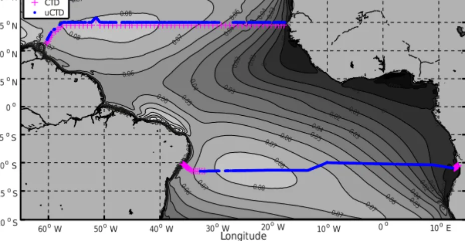
Two trans-Atlantic zonal sections near 14.5^◦N and 11^◦S were occupied by R/V Meteor on three cruise legs (M96, M97, and M98). The 14.5^◦N section began with cruise M96 off the coast of Trinidad and Tobago on 28 April 2013. The section ended on M96 at about 20^◦W on 20 May, and was continued to the African coast during M97 from 8 to 9 June (Fig. 1). During these surveys, 64 CTD stations were conducted along the 14.5^◦N section, with an average spacing of 40 nm (75 km). Parallel to the CTD system, the uCTD system was operated between the adjacent CTD stations when the ship was steaming at 10–12 kn. In total, 317 uCTD profiles were achieved, with an average spacing of 8 nm (15 km).

The 11^◦S section was surveyed during M98 from 6 to 23 July 2013. In this section, the standard CTD was only operated on the shelf and at the shelf break; during the transit across the Atlantic, only the uCTD was in use. All together, 290 uCTD profiles were taken during the survey, with an average spacing of 11 nm (20 km). Shipboard ADCP and anemometer were in continuous operation through the entire cruises.

2.1 CTD and uCTD measurements

The CTD work was carried out with a Sea-Bird Electronic (SBE) 9 plus CTD system. The two temperature sensors were calibrated at the manufacturer just before cruise M96 in March 2013. The conductivity measurements were calibrated by comparing the bottle stop data with salinometer measurements of bottle samples. All CTD system quality control pro- cedures followed the GO-SHIP recommendations (Hood et al., 2010). The accuracy of the CTD data was estimated to be

±0.001^◦C for temperature and±0.002 g kg⁻¹for salinity.

The uCTD system used at both zonal sections was an Oceanscience Series II underway-CTD. It consisted of a probe, a tail, and a winch. The probe is equipped with a temperature (SBE-3F), a conductivity (SBE-4) and a pressure sensor from SBE. A tail spool reloading system allows the rope spooled on the tail to be paid out when the probe falls

(4)

60ôW 50ôW 40ôW 30ôW 20ôW 10ôW 0ô 10ôE 20 ôS

15 ôS 10ôS 5 ôS 0ô 5 ôN 10ôN 15ôN 20ôN

−0.03

−0.03 −0.02

−0.02

−0.02 −0.01

−0.01

0

0 0

0.01

0.01 0.01 0.01

0.01

0.02

0.02 0.02 0.02

0.02

0.03

0.04

0.04 0.04

0.05

0.05 0.05

0.06 0.06

0.06

0.06 0.06

0.07

0.07 0.07

0.07

0.07 0.08

0.08 0.08

0.08

0.070.08 0.08

0.10.09 0.1

0 0

Longitude

Latitude

CTD uCTD

Figure 1.Positions of the CTD (magenta+) and uCTD (blue dots) measurements along the 14.5^◦N and 11^◦S sections. The 14.5^◦N section was completed during RVMeteorcruises M96 (28 April to 20 May 2013, west of 20^◦W) and M97 (8 to 9 June 2013, east of 20^◦W), the 11^◦S section during M98 (6 to 23 July 2013). Note that the uCTD position for the 14.5^◦N section is artificially shifted to the north by 0.5^◦ for visual clarity. The grey shading with contours is the mean zonal wind stress calculated from NCEP/CFSr monthly wind stress between 1979 and 2011 in N m⁻².

Table 1.Meridional Ekman volume (M^yin Sv), heat (H_ein PW), and salt (S_ein 10⁶kg s⁻¹) fluxes calculated using different methods, and the transport-weighted temperature2_Eand salinityS_AEin the Ekman layer. Positive and negative fluxes denote northward and southward fluxes, respectively. The uncertainties of the Ekman heat and salt flux are 0.4 PW and 45×10⁶kg s⁻¹at 14.5^◦N, and 0.3 PW and 65×10⁶kg s⁻¹ at 11^◦S, respectively. The uncertainties of the transport-weighted Ekman temperature and salinity are 0.20^◦C and 0.15 g kg⁻¹at 14.5^◦N, and 0.11^◦C and 0.10 g kg⁻¹at 11^◦S, respectively.

Section

14.5^◦N 11^◦S

2_E S_AE M^y He Se 2_E S_AE M^y He Se

Method

Direct TTP/profile 25.52 36.33 6.21 0.413 5.40 25.41 36.83 −11.71 −0.842 −17.69 TTP/surface 25.61 36.34 6.21 0.415 5.49 25.41 36.80 −11.71 −0.842 −17.38 TTP 25.46 36.32 6.68 0.443 5.72 25.13 36.81 −13.64 −0.965 −20.50 Indirect Surface 25.65 36.29 6.68 0.448 5.57 25.20 36.78 −13.64 −0.946 −20.04 Annual 26.46 36.13 8.31 0.584 5.56 25.53 36.73 −11.02 −0.799 −15.49

freely. The sensors record data at a frequency of 16 Hz. For most of the profiles about 250–300 m of rope were spooled on the tail spool (which set the fall depth) and the recording time length was set to 100 s, and about 1600 data recordings per cast were obtained. From the tail spool the probe sinks freely with a nominal speed of 4 m s⁻¹. However, due to the back-and-forth unspooling of the rope from one end of the tail to the other, the sinking speed typically varies from 3 to 4.5 m s⁻¹. After the rope on the tail is paid out completely, the probe still sinks at speeds less than 2 m s⁻¹in the last tens of metres of its sinking before being winched back to the ship and recovered back to deck. Three probes were used during the two section surveys (nos. 70200126 and 70200068 along the 14.5^◦N section; nos. 70200068 and 70200138 along the 11^◦S section). The uCTD winches were out of service several times during the three cruise legs. Although they were

repaired on-board, several measurement gaps were left, for example, between 29 and 27^◦W (Fig. 1).

The post-calibration of the uCTD data was done in two major steps: the first step is a sensor calibration procedure, which corrects the temperature sensor error due to viscous heating, the conductivity sensor error due to thermal mass delay, and the lag between the conductivity and temperature sensors; the second step is data validation in reference to CTD profile data and to thermosalinograph (TSG) data. The first step was done following Ullman and Hebert (2014) (hereafter UH2014). We will briefly describe the pro- cess here; for details, please refer to their work. The uCTD is an unpumped CTD system, the rapid sinking speed of 4 m s⁻¹ allowing water to pass through the sensor package at 3.56 m s⁻¹(UH2014). This flow rate is much higher than a pumped CTD system (1 m s⁻¹), which leads to a clear viscous heating effect of the uCTD temperature sensor. This was

(5)

corrected using a steady-state result of Larson and Pedersen (1996) for the perpendicular flow case (cf. Eq. 8 of UH2014).

The thermal mass correction was performed following the al- gorithm of Lueck and Picklo (1990) and using the mean values of error magnitude and time constant from UH2014 (cf.

Table 1 of UH2014).

From the uCTD profiles alone a time lag correction was determined from cross-correlation of temperature and conductivity sensor small-scale variability. The variability was calculated by subtracting a sixth-order Butterworth low-pass filtered profile with a cut-off frequency of 4 Hz from the corresponding temperature and conductivity time series of each profile. The highest correlation was found for a 1/16 s lag (conductivity leading), which equals the sampling frequency of 16 Hz data. Application of the lag eliminated most of the spikes in the salinity profiles when the sinking speed of the probe was above about 1.5 m s⁻¹. However, when the sinking speed was below 1.5 m s⁻¹, this correction would cause the spikes pointing in the opposite direction and indicates an inverse dependency of the lag on the sinking speed. This result is consistent with that reported by UH2014, and we corrected the lag following their lag model (cf. Eq. 7 of UH2014), but adjusted their parameters to match our data. The data recorded with a sinking speed smaller than 0.3 m s⁻¹ were neglected (including all upcast data).

Validation of the lag corrected uCTD against CTD profile data revealed for the 14.5^◦N section a drift in the conductivity sensors of uCTD probes nos. 70200126 and 70200068.

A bias correction in the sense of an absolute salinity offset (uCTD–CTD) was determined based on the temperature–

salinity space (Rudnick and Klinke, 2007) by considering the conservative temperature range from 12 to 14^◦C and using all uCTDs between adjacent CTD pairs. This particular temperature range was chosen because it belongs to the Atlantic central water, whoseT /Srelation is nearly linear, which implies that in this temperature range, the spreading of salinity measured during different uCTD casts should be tight. Be- sides, it was also surveyed by almost all uCTD casts along the section. For probe no. 70200126, the salinity offset fluc- tuates around a mean value of 0.038 g kg⁻¹west of 39^◦W (CTD station 34), east of which the offset shifts abruptly to around 0.151 g kg⁻¹. The calibration was done by applying the mean offset values to the salinity data in the corresponding groups of uCTDs. The salinity data of the last few profiles of probe no. 70200126 (between 30 and 29^◦W) were extremely noisy, and not possible to calibrate. This probe was not further used during the rest of the section due to its poor quality of the salinity data. For probe no. 70200068, the salinity offset remains around 0 west of 36^◦W (CTD station 38), and then abruptly shifts to around 0.295 g kg⁻¹between 36 and 23.5^◦W (CTD station 56). East of 23.5^◦W to the African coast, the offset shows a linear decreasing trend. This is likely due to the increasing portion of South Atlantic central water (SACW) in the central water layer when approaching the coastal region, which is less saline than the North At-

lantic central water (NACW), and consequently shifting the slope of theT /S curve. As a result, the linear trend of the offset east of 23.5^◦W should not be due to instrument error.

Therefore, only a mean offset was calculated and applied to calibrate each corresponding group of profiles made by no.

70200068. The reasons for the abrupt drift in the salinity (as obtained from the conductivity sensors) are not clear, but it is likely that due to the repeated intensive usage, the conductivity sensors were contaminated or impacted (hit ship hull).

The shipboard TSG provides another source of validation and calibration of uCTD data. On R/V Meteor, the TSG (SBE38 for temperature sensor, SBE21 for conductivity sensor) measures temperature and salinity at an intake at approximately 6.5 m depth. For all three legs, the TSG conductivity cell was calibrated from salinity analysis of water samples taken at the water intake, and a comparison with CTD data (if available) was also done. The uCTD salinity calibration was done by calculating the conductivity offset between the uCTD at 6.5 m and the averaged TSG conductivity within 5 min before and after the uCTD down- cast. For probe no. 70200126, the drift of its conductivity sensor manifests also east of 39^◦W, the conductivity offset west of 39^◦W is about−0.022 S m⁻¹, and east of that it is about 0.094 S m⁻¹. These differences in conductivity correspond to a change in salinity of−0.015 and 0.08 g kg⁻¹, respectively. For probe no. 70200068, the conductivity offset west of 36^◦W is indistinguishable from zero, while east of that it is 0.156 S m⁻¹, which corresponds to a salinity difference of 0 and 0.15 g kg⁻¹. No trend in the offset east of 23.5^◦W is detected. For the 14.5^◦N section, we had uCTD, CTD, and TSG data available and the respective calibrations uCTD/CTD and uCTD/TSG could be compared. This was done in order to see if in case only TSG data are available (as is the case for the 11^◦S section), still reasonable calibration results could be achieved. For both probes, the TSG- derived drifts occurred in the same longitude range as they were detected using the CTD data. However, the magnitude of the offset was generally smaller for the TSG compared to the CTD-based method, especially for probe no. 70200126 in the longitude range west of 39^◦W, where even the signs of the offsets were opposite to each other. Such a difference is likely due to the fact that the CTD-based method employs a specific conservative temperature range where the salinity variation is small, while the TSG-based method focuses only at near-surface values (6.5 m), where the salinity varies in a broad range. Therefore, we would trust more the CTD- based method, and note that if the TSG-based method returns a small conductivity offset (<0.03 S m⁻¹), one might need more caution to apply this offset to calibrate the uCTD.

However, one needs also more caution when applying the CTD-based calibration in regions, where the T /S relation of the central water shows a mixture effect of NACW and SACW. At the 11^◦S section, CTD data were only available at the beginning and end of the section; we could use only the TSG data as the primary source for validation. Fortu-

(6)

nately no drift was detected in the uCTD probes’ conductivity cell, but a stable offset with a mean value of 0.131 and 0.073 S m⁻¹ was detected and applied for probes nos.

70200068 and 70200138, respectively.

After the offset/drift calibration, all the uCTD data were gridded vertically from the original resolution (∼0.25 m at a nominal sinking speed of 4 m s⁻¹) to 1 m for the geostrophic velocity calculation later. Following Rudnick and Klinke (2007), we estimated that the calibrated and gridded uCTD data have an accuracy of 0.02–0.05 g kg⁻¹ in salinity and 0.004^◦C in temperature.

All calculations in this study are based on the Thermody- namic Equation of State for seawater 2010 (TEOS-10, Mc- Dougall and Barker, 2011). TEOS-10 is introduced to replace the previous Equation of State, EOS-80, and it provides a thermodynamically consistent definition of the equation of state in terms of the Gibbs function for seawater. The most obvious change in TEOS-10 is the adoption of conservative temperature (2) and absolute salinity (S_A) to replace the potential temperature and practical salinity. Although the new equation of state has a non-negligible effect on the density field in the deep ocean, its effect in the upper ocean is expected to be small; therefore, our results obtained using TEOS-10 should be comparable with the previous studies.

2.2 ADCP measurements

Direct current velocity profiles were measured continuously during all three cruise legs with vessel-mounted 75 and 38 kHz Teledyne RDI Ocean Surveyors (OS75 and OS38).

The OS75 was configured to measure at a rate of 2.2 s and a bin size of 8 m. The measurement range varied between 500 and 700 m. The OS38 was set to measure at a rate of 3.5 s and at 16 m (32 m) bin size during the 14.5^◦N (11^◦S) section. The measurement range was mostly 1200 m. Ship navigation information was synchronized to the ADCP system.

The misalignment angles and amplitude factors were calibrated during post-processing. The processed data contain 10 min averaged absolute velocities in earth coordinates; the first valid bin for OS75 is centred at 18 m at 14.5^◦N and 13 m at 11^◦S, for OS38 is 21 m at both sections. In this study, only the OS75 velocity was used since it has a higher accuracy in upper layers and higher vertical resolution. The uncertainties of 1 h averages were estimated by Fischer et al. (2003) to be 1–3 cm s⁻¹.

Wind data

We used three different wind datasets in our analysis. First, we used the observed wind speed and direction recorded with the R/V Meteoranemometer, mounted at a height of 35.3 m. The wind data were stored with a temporal resolution of 1 min. True wind speed and direction were calculated using ship speed and direction from the navigation system.

On-station measurements were removed. The reduction from

the observation height to 10 m standard height was calculated according to Smith (1988) and wind stress was calculated according to Large and Yeager (2004) assuming neutral stabil- ity. The final wind stress used for the Ekman transport calculation was binned in 50 km ensembles to filter out small-scale variability.

The blended Satellite-based level-4 Near-Real-Time wind stress product (hereafter satellite wind stress) from the Copernicus Marine Environment Monitoring Service (CMEMS) was used. The wind speed data are derived from retrievals of scatterometers aboard satellite METOP- A (ASCAT) and Oceansat-2 (OSCAT) and combined with the European Centre for Medium-Range Weather Fore- casts (ECMWF) operational wind analysis and gridded to 0.25^◦×0.25^◦resolution in space and 6 h in time. The wind stress data were estimated using the COARE 3 model (Fairall et al., 2003).

Moreover, the NCEP/NCAR monthly zonal wind stress at 14.5^◦N and 11^◦S corresponding to the months of the cruises (i.e. May and July 2013) was used to calculate the Ekman transport.

2.3 GECCO2 ocean synthesis data

In order to integrate our local observational results into a large-scale circulation, the GECCO2 ocean synthesis data were used and compared (Köhl, 2015). GECCO2 is a Ger- man version of the MIT general circulation model “Es- timating the Circulation and Climate of the Ocean system” (ECCO, Wunsch and Heimbach, 2006). It has 1^◦×¹

3

◦

resolution and 50 vertical levels. GECCO2 includes the Arctic Ocean with roughly 40 km resolution and a dy- namic/thermodynamic sea ice model of Zhang and Rothrock (2000). The synthesis uses the adjoint method to bring the model into consistency with available hydrographic and satellite data (Köhl, 2015). The prior estimate of the at- mospheric state is included by adjusting the control vector, which consists of the initial conditions for the temperature and salinity, surface air temperature, humidity, precipitation and the 10 m wind speeds from the NCEP RA1 reanalysis 1948–2011 (Köhl, 2015). The surface fluxes are derived by the model via bulk formulae of Large and Yeager (2004). For the study period from May to July 2013 monthly and daily output data were available. It is important to note that the in situ observational data measured during the cruises were not assimilated in the synthesis, while the satellite measured wind speed was assimilated but possibly modified via the synthesis.

3 Methods

According to Eqs. (1) and (2), the meridional Ekman volume transport can be calculated from zonal wind stress data, as well as from observed ageostrophic velocity. Hereafter

(7)

we refer to the wind-stress-based calculation as the “indirect method”, and to the ageostrophic-velocity-based calculation as the “direct method”. In this section, we describe some details of the geostrophic and ageostrophic velocity calculation, the definition of the penetration depth of the Ekman flow, the error estimate of the direct Ekman transport calculation, and different methods to derive the Ekman heat and salt fluxes.

3.1 Geostrophic and ageostrophic velocity calculations According to the thermal wind relation, relative geostrophic velocity referenced to the velocity at the reference depth can be calculated from the density field measured by the CTD and uCTD. At 14.5^◦N, two sets of the relative geostrophic velocity were calculated independently from the CTD and uCTD datasets. For CTDs, the relative geostrophic velocity referenced to 200 m was computed between the adjacent stations (average distance about 75 km). For uCTDs, in order to take advantage of the high spatial resolution, the relative geostrophic velocity to 200 m was calculated between any closest pair of uCTD profiles with a minimum distance of 70 km (roughly the Rossby radius of deformation at this latitude). Along the 11^◦S section, CTD profiles were only taken in the vicinity of the coasts, and over most of the section only uCTD data are available (Fig. 1). Therefore the geostrophic velocity was computed from the combined CTD and uCTD dataset following the methodology applied to uCTD data at the 14.5^◦N section, except that at 11^◦S the minimum distance between the closest profiles was set to 90 km (roughly the Rossby radius of deformation at 11^◦S). Note that the distance between uCTD profiles for geostrophic velocity calculation is an arbitrary choice, and varying the distance from 70 to 110 km has a negligible effect on the total transport (less than 2 %).

To obtain the absolute geostrophic velocity, the reference velocity at 200 m was obtained from the ADCP measurement. The ADCP velocity was projected to the normal direction of the cruise track and then averaged between the corresponding CTD/uCTD pairs. We did not include the ADCP velocity data recorded at the CTD stations, because velocity was repeatedly measured at a CTD station; zonally averaging the ADCP velocity would bias the result towards the on-station velocity. In previous studies (Wijffels et al., 1994; Chereskin et al., 1997; Garzoli and Molinari, 2001), the corresponding ADCP velocity at the reference depth was taken as the reference velocity, assuming that the flow at the reference depth was in geostrophic balance.

However, the section-averaged ADCP velocity profile for the 14.5^◦N section shows a complicated vertical structure (Fig. 3a) and it is not obvious at which depth the flow is approximately in geostrophic balance. Thus, referencing the relative geostrophic velocity to the ADCP velocity only at a chosen depth may lead to a biased absolute geostrophic velocity. As a result, the ageostrophic velocity may be sen- sitive to the choice of the reference level. To overcome this

problem, a reference velocity was calculated as an averaged offset between each relative geostrophic velocity and the corresponding ADCP velocity within a common depth range, over which the ageostrophic components are averaged to about 0. This averaged offset should represent the absolute geostrophic velocity at the reference depth and is roughly independent of the vertical variation due to the ageostrophic components. At 14.5^◦N, the common depth range for the CTD-based calculation is between 70 and 500 m, which is expected to be below the surface Ekman layer and covered by both CTD and ADCP measurement. Due to the limitations in the maximum deployment depth, the uCTD-based calculation covers the depth range between 70 and 250 m.

At 11^◦S the depth range is between 100 and 300 m, which should also be below the Ekman layer and was covered by the uCTD and ADCP measurement.

The ageostrophic velocity was then calculated as the difference between the ADCP velocity and the absolute geostrophic velocity. Note that the choice of the depth range still affects the reference velocity due to the vertical variation in the ADCP meridional velocity. For example, using a depth range between 70 and 250 m for the CTD-based calculation (same as the uCTD depth range) would decrease the final ageostrophic velocity by 0.44 cm s⁻¹; using another depth range would not result in an absolute difference ex- ceeding this value. This is much smaller compared to the uncertainty caused by using the ADCP velocity at a single depth as the reference velocity (up to 1.75 cm s⁻¹), as can be anticipated from the section-averaged meridional ADCP velocity (Fig. 3a). The sensitivity of the absolute geostrophic velocity to the choice of the reference level was also tested at 14.5^◦N. Changing the reference level from 150 to 250 m would make a change in the absolute geostrophic velocity indistinguishable from zero.

3.2 Penetration depth of the Ekman flow

Because the ocean is not homogenous, a control surface must be defined that characterizes the maximum penetration depth of the momentum flux into the upper ocean. One choice would be the MLD, which we defined as the depth where the density increased by 0.01 kg m⁻³in reference to the value at 10 m (following Wijffels et al., 1994). Along both sections, the MLD is relatively shallow (on average 25.1 m at 14.5^◦N and 32.2 m at 11^◦S), and as such unlikely a representative ofDE (Figs. 3 and 4). According to the Ekman theory,DE

for water at 14.5^◦N with a typical vertical eddy viscosityAv

of 0.02 m²s⁻¹would be 33.1 m (see the definition ofDEin Eq. 1).

Alternatively a TTP has been defined as the shallowest depth at which the density gradient is larger than 0.01 kg m⁻⁴ (Wijffels et al., 1994). The TTP is typically deeper than the MLD and better defines the transition depth between well- mixed and stratified ocean, up to which the momentum from the wind is transferred (Chereskin et al., 2002). At some lo-

(8)

cations along both sections we observed two homogenous layers of slightly different density and possibly a remnant of the seasonal mixed layer cycle. In these cases, the TTP depth was chosen as the deeper one of the depth that sat- isfies the density gradient criterion. Since TTP was defined based on a gradient criterion, it represents the bottom of a weakly stratified surface layer rather than a specific density surface. Along the 14.5^◦N section, the mean TTP depth is 45.8 m (Fig. 3a). At both ends of the section, the TTP coin- cides with the MLD and is relatively shallow, while in the remaining part of the 14.5^◦N section TTP is deeper than the MLD (Fig. 4c). Along the 11^◦S section, the mean TTP depth is 56.8 m, and the TTP is deeper than the MLD throughout the section (Figs. 3b and 4d).

3.3 Error estimate of the direct Ekman transport The errors of the direct Ekman transport were estimated following Chereskin and Roemmich (1991) and Wijffels et al. (1994). Assuming that near-inertial motions are the dom- inant source of error, decorrelation length scales were calculated as the distance that the ship travelled in a quarter of the inertial period at 14.5^◦N (47.9 h) and 11^◦S (62.7 h) resulting in 130 and 230 km, respectively. In total, 38 segments of the 14.5^◦N section and 25 segments of the 11^◦S section were obtained by dividing the total distance of each section by the corresponding decorrelation length scale, respectively. The westernmost and easternmost four segments of each section were omitted because of the anomalously weak wind near the eastern boundary and the strong boundary current in the western boundary region. The degree of freedom (DOF) of 30 and 17, respectively, was the number of the remaining segments. The ageostrophic transport within each segment was treated as an independent realization of the Ekman transport.

Therefore, standard errors were calculated. Then the final error is given as the standard error times the DOF. Another fac- tor that could lead to an uncertainty is the depth range used to calculate the reference velocity from the ADCP velocity.

As discussed above, we argue that the vertical structure of the ageostrophic velocity should arise from the near-inertial motion and therefore, should be included already in this uncertainty estimate.

3.4 Ekman heat and salt flux calculation

The Ekman heat and salt fluxes, He and Se, respectively, were calculated by combining the indirect and direct Ekman volume transport estimates with 2 and SA from different sources. Note that in order to calculate the Ekman fluxes in the context of mass conservation (Montgomery, 1974), it has to be assumed that the Ekman volume transport in the upper layer is balanced by an equal and opposite geostrophic return flow at depth. This is a reasonable assumption and has been routinely adopted in many inverse studies (Ganachaud and Wunsch, 2003). To account for this return flow, an averaged

conservative temperature,2, and absolute salinitySA were subtracted from the in situ2andSAat each section.2and SAare the zonally and vertically (0–5000 m) averaged conservative temperature and absolute salinity, calculated from the annual climatology of the World Ocean Atlas 2013 v2 (Locarnini et al., 2013; Zweng et al., 2013) at each section.

In the following, the calculation details of the Ekman heat flux and transport-weighed Ekman temperature are given; the calculation of the Ekman salt flux and transport-weighted Ek- man salinity is an analogue.

3.4.1 Direct methods

By using the in situ2together with the ageostrophic velocity within the layer from the sea surface to the TTP (referred to as the TTP layer), the Ekman heat fluxHe was calculated (referred to as the direct TTP/profile).

H_e=ρC_p Z x2

x₁

Z 0

−TTP

2 (x, z)−2

v_ageo(x, z)dzdx, (3) whereC_p is the specific heat capacity of sea water at constant pressure,ρ is the density of sea water, in this study we assumed a constantCp=4000 J kg⁻¹K⁻¹and a constant ρ=1025 kg m⁻³,vageois the ageostrophic velocity,2is the in situ conservative temperature.2is the mean conservative temperature at the corresponding section.

It is useful to consider the Ekman heat flux as the product of the Ekman volume transport,M^y, and the transport- weighted temperature,2_E. The transport-weighted temperature then can be calculated as follows:

2E= Rx₂

x1

R0

−TTP2 (x, z) v_ageo(x, z)dzdx

M_direct^y . (4)

As a comparison to the direct TTP/profile method, the Ekman heat fluxes using only in situ SST from the CTD and uCTD were also calculated (referred to as the direct TTP/surface).

This was done by replacing the in situ2(x, z) in Eqs. (3) and (4) with the in situ SST2 (x, z=0).

The uncertainty of the direct Ekman heat and salt fluxes was estimated following Chereskin et al. (2002). Since the wind direction was predominantly uniform and westward, the uncertainty should mainly arise from the ageostrophic velocity that was opposite to the expected Ekman flow direction. Therefore, the uncertainty was calculated still using Eqs. (3) and (4), except that only southward or northward ageostrophic velocity was used in both the numerator and denominator for the 14.5^◦N or 11^◦S section, respectively.

3.4.2 Indirect surface method

Often Ekman heat and salt fluxes are estimated by combining the Ekman volume transport inferred from wind stress with the SST and sea surface salinity (SSS) from a climatology or satellite measurements (e.g. McCarthy et al., 2015). Here,

(9)

we calculated the heat flux using in situ wind and in situ SST data (referred to as the indirect surface) to compare with the direct estimates. Additionally, annual Ekman heat and salt fluxes (referred to as the indirect annual) were calculated using an annual average of the monthly NCEP/NCAR reanalysis wind stress data between 1991 and 2013 and the annual average of SST and SSS from the Roemmich and Gilson (2009) monthly Argo climatology (hereafter RG climatology). Following Levitus (1987), the Ekman heat flux for the indirect surface method was calculated as

H_e=C_p Z

2(x, z=0)−2τx

f dx, (5)

whereτ_xis the in situ wind stress in the tangential direction of the cruise track,f is the Coriolis parameter, and2(x, z= 0)is the in situ SST. The transport-weighted temperature was calculated as follows:

2_E=

R2(x, z=0)_ρf^τ^xdx

M_indirect^y . (6)

The indirect annual method is an analogue to the indirect surface method, except that the Ekman volume transport and SST were derived from the NCEP/NCAR reanalysis wind stress and RG climatology, respectively.

3.4.3 Indirect TTP method

Wijffels et al. (1996) assumed a linear Ekman velocity profile between the surface and TTP and calculated the Ekman heat and salt fluxes using climatological wind stress data, combined with the in situ temperature and salinity. Here we followed their method and used the in situ2,SA, and wind to calculate the Ekman heat and salt fluxes (referred to as the indirect TTP) as a counterpart to the direct TTP method.

He

=Cp

Z h2

32 (x, z=0)+1

32 (x, z=TTP)−2 iτx

f dx, (7) where2 (x, z=TTP)is the in situ conservative temperature at TTP depth from the CTD/uCTD. The transport-weighted temperature was calculated as follows:

2E= Rh

2

32 (x, z=0)+¹

32 (x, z=TTP)i

τx

ρfdx

M_indirect^y . (8)

4 Results and discussion

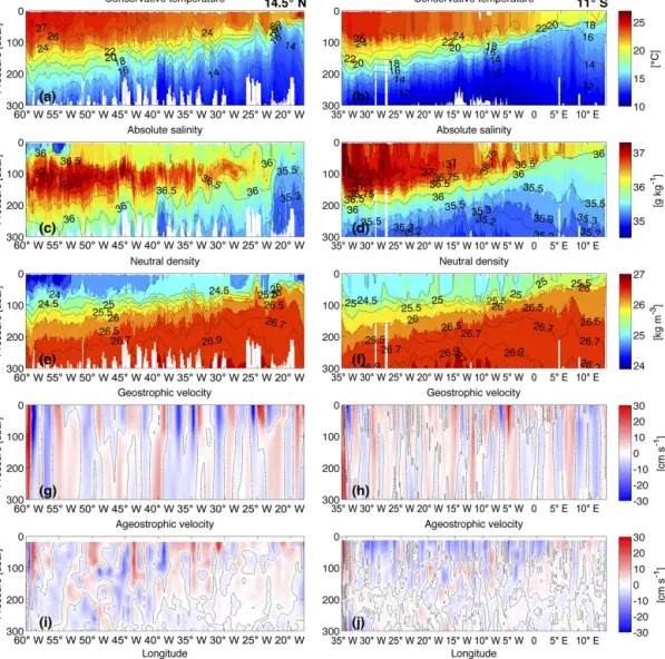
4.1 Upper layer hydrography at 14.5^◦N and 11^◦S Along both sections (Fig. 2a, b) the typical upward tilting of isotherms towards the east, as a result of the subtropical gyre circulation, can be seen. Along the nominal 14.5^◦N section, the water in the upper 50 m, compared to that at 11^◦S, was relatively warm and fresh, with an averaged2 and S_A of about 26.03^◦C and 36.15 g kg⁻¹, respectively. The minimum S_Acore near the western boundary probably originates from the freshwater runoff from the Amazon River (Fig. 2c). To- gether with the warm temperature, it forms the lightest water observed along the section (Fig. 2e). A subsurface salinity maximum layer of Subtropical Underwater (STUW) is centred at 100 m depth withSAgreater than 37.2 g kg⁻¹. STUW is formed in the subtropical Atlantic with a SSS maximum due to excessive evaporation, and is subducted equatorward (Talley et al., 2011). The upward tilt of the isopycnals from west to east is suggestive of a net southward geostrophic transport when excluding the western boundary, where sharp deepening of the isopycnals implies a northward, intensi- fied boundary current (Fig. 2g). At 11^◦S, the surface water was cooler and more saline than that at 14.5^◦N, with an averaged2andS_A of about 24.52^◦C and 36.69 g kg⁻¹. The STUW with maximum salinity larger than 37.3 g kg⁻¹ was centred at about 100 m, but was even saltier than that at 14.5^◦N. Likewise, a net northward geostrophic flow can be anticipated from the displacement of the isopycnals. At the western boundary, the North Brazil Undercurrent (NBUC) is characterized by a narrow and strong northward velocity band west of 35^◦W (Schott et al., 2005) (Fig. 2h). In the hydrographic data2/S_A variability is seen at both sections that are associated with mesoscale eddies. For instance, at 14.5^◦N/25^◦W and 11^◦S/7^◦E, cyclonic and anticyclonic eddies were characterized by the upward peak of the isotherms, and were clearly visible from the geostrophic velocity sections (Fig. 2g, h).

The daily2andS_A data of the GECCO2 synthesis were extracted from the model grid to the nearest time and position of the ship measurement. In general, GECCO2 daily data re- produced the observed hydrographic structure very well (not shown). The upward tilt of the isopycnals from the west to the east and the subsurface salinity maximum withSAlarger than 37.2 g kg⁻¹ were clearly captured by GECCO2. How- ever, the most obvious difference was at the western boundary of 11^◦S, where the surface salinity was not as high as the observed values, and the isopycnals were not tilting in the same direction, indicating that the shallow western boundary current in the GECCO2 flowed in the opposite direction compared to the observation at 11^◦S. But we expect that this difference should not impact the ageostrophic velocity calculation, since the geostrophic velocity must be removed from the total velocity.

(10)

Figure 2.Vertical sections of conservative temperature in^◦C(a, b), absolute salinity in g kg⁻¹(c, d), neutral density in kg m⁻³(e, f), geostrophic velocity in cm s⁻¹(g, h), and ageostrophic velocity in cm s⁻¹(i, j)at 14.5^◦N (left) and 11^◦S (right). All the available CTD and uCTD data were used to produce(a–f), and the contours were plotted with every fifth value for visual clarity.(g)and(i)were calculated using only CTD data, while(h)and(j)were calculated using CTD and uCTD data. The blanks were due to the shallow measurement depth of the uCTD.

4.2 Vertical structure of the ageostrophic flow

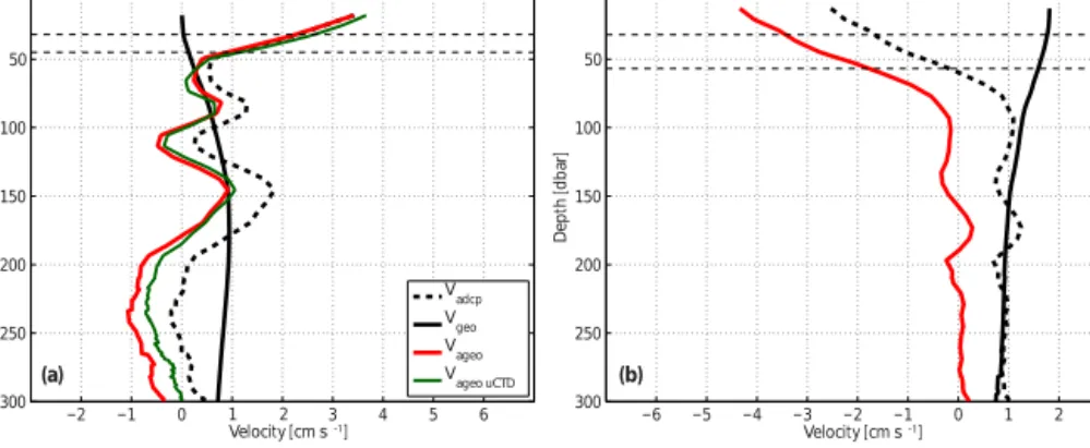
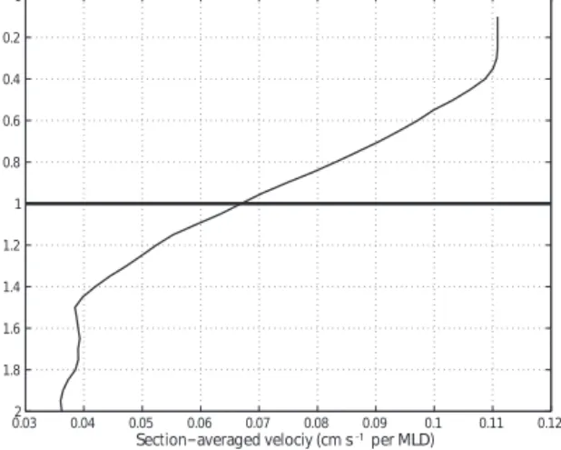
Although northward (southward) ageostrophic velocity at 14.5^◦N (11^◦S) dominates the upper 50–70 m (Fig. 2i, j), as expected from the persistent westward trade winds, the appearance of southward (northward) velocity at 14.5^◦N (11^◦S) in the upper 50–70 m and below indicates the existence of non-Ekman ageostrophic components in the water column. This will be discussed in detail below. The section- averaged ageostrophic velocity based on CTD data at 14.5^◦N shows a relatively complicated vertical structure with multi- ple maxima and minima (Fig. 3a). It has a northward maximum velocity of 3.5 cm s⁻¹near the surface, and decreases to about 0.3 cm s⁻¹at about 60 m, followed by a minor peak at about 80 m before approaching 0 at 100 m. Another peak

of 1 cm s⁻¹ appears at about 150 m, and below 180 m the velocity changes direction. When the ageostrophic velocity is calculated based on the uCTD data, it has a very consistent structure and strength compared to the CTD-based ageostrophic velocity (Fig. 3a). This is meaningful information as the hydrographic data at 11^◦S consist primarily of uCTD data. The good agreement between the CTD and uCTD data analysis at 14.5^◦N justifies the use of either one or the other. At 11^◦S, the ageostrophic velocity shows a near- surface southward maximum of 4.3 cm s⁻¹, decreases almost linearly in the upper 70 m, and gradually approaches 0 at about 100 m (Fig. 3b). In contrast to the northern section the vertical variations of the ageostrophic velocity profile below 100 m are very small.

(11)

−2 −1 0 3 4 5 6 0

50 100 150

200 250

300 (a)

1 2 Velocity [cm s^-1]

Depth [dbar]

V_adcp V_geo V_ageo V_{ageo uCTD}

−6 −5 −4 −3 −2 −1 0 1 2

0

50 100 150

200 250

300 (b)

Velocity [cm s^-1]

Depth [dbar]

Figure 3.Section-averaged cross-track velocity profiles at(a)14.5^◦N and(b)11^◦S. In(a), the solid red curve and the solid black curve are the ageostrophic and geostrophic velocity calculated from the CTD data, respectively. The dark green curve is the ageostrophic velocity profile based only on the uCTD data. In(b), the solid red curve and solid black curve are the ageostrophic and geostrophic velocity calculated from the combination of the CTD/uCTD data, respectively. The dashed black curve is the ADCP velocity. The upper horizontal dashed line denotes the basin-wide averaged MLD and the lower one denotes the basin-wide averaged TTP depth.

Figure 4.Vertical sections of residual meridional velocity in cm s⁻¹at(a)14.5^◦N and(b)11^◦S and of buoyancy frequency calculated from uCTD/CTD at(c)14.5^◦N and(d)11^◦S. Northward velocity in(a, b)is shaded in red, southward in blue. The residual velocity is calculated by subtracting an 80 m boxcar filtered profile from the original ADCP profile. The white circles in(c, d)denote the MLD; the black triangles denote the TTP (see text for details). The MLD and TTP plotted here are subsampled for visual clarity. Note that no uCTD measurements were conducted between 30 and 25^◦W at 14.5^◦N.

Assuming that the Ekman balance would hold true along the analysed sections, the ageostrophic velocity would decrease undisturbed from its surface maximum to about 0 at a certain depth (Ekman depth, D_E). However, the observed wave-like structure at 14.5^◦N indicates that other processes must play a role in setting the section mean ageostrophic flow field. To identify this wave-like structure, we tried to separate the non-Ekman ageostrophic flow from the other components by using the ADCP velocity. A residual velocity was calculated by subtracting an 80 m boxcar filtered velocity profile from the original ADCP meridional velocity (Fig. 4a, b).

The 80 m filter window was determined based on the vertical length scale of the wave-like structure in the section- averaged ageostrophic velocity profile by visual inspection.

At 14.5^◦N, vertically alternating structures with wavelengths of 60–80 m are clearly visible, are coherent and persistent throughout the section, and are most pronounced between 52 and 46^◦W (Fig. 4a). At 11^◦S, similar signals are visible for most of the section, but are not as strong as at 14.5^◦N (Fig. 4b).

Zonally averaging the residual velocity results in a velocity profile with a vertically alternating structure similar to that in the section-averaged ageostrophic velocity in both strength and structure, indicating that the vertical variation in the ageostrophic velocity mainly arises from the presence of high-order baroclinic waves. Figure 4c and d show the buoyancy frequency (N²) for the two sections, respectively. It appears that the wave-like signals occur mainly in the strongly

(12)

stratified layer (pycnocline) marked by high N²values.N² is calculated as follows:

N²= g ρ0

∂ρ(z)

∂z , (9)

wheregis the gravitational acceleration,ρ₀=1025 kg m⁻³ is the reference density, andρ (z)is the in situ potential density as a function of depth,z.ρ (z)was calculated by using a combination of CTD and uCTD profile data with a re-gridded vertical resolution of 5 m at both sections.

Chereskin and Roemmich (1991) also observed energetic, circularly polarized, relative currents of large horizontal co- herence below the base of the mixed layer at 11^◦N in the At- lantic. They described the signal as the propagation of near- inertial internal waves and argued that the presence of a near- inertial peak in internal wave spectra, together with continuously varying wind forcing, would guarantee the appearance of these waves. Using satellite-based wind stress data, we ex- amined the changes in wind stress at the measurement points within the last 2 weeks before the ship arrived at the measurement points. Although the wind stress strongly changed along the whole section, it is still not indicative why the wave signal is strongest between 52 and 46^◦W at 14.5^◦N. It is tempting to believe that these waves are near-inertial internal waves. However, due to the fact that the ship moved nearly constantly except when it was on station, it is extremely dif- ficult to identify what exactly these signals are. More so- phisticated methods may be applied to analyse the wave-like signal; for instance, Smyth et al. (2015) took the Doppler shift in the shipboard current measurement into account, and translated observed Yanai wave properties into the reference frame of the mean zonal flow. But this is obviously beyond the scope of this work.

4.3 Ekman transport 4.3.1 Indirect method

According to Eq. (1), the Ekman transport can be calculated from the wind stress data (referred to as the indirect method) by integrating the left-hand side of Eq. (1) zonally. The in situ wind stress data and a satellite-based wind stress product from CMEMS were used. The satellite wind stress data were extracted from the original grid to the nearest time and nearest position of the ship navigation. Both in situ and satellite wind stress were projected to the tangential direction of the cruise track, so that the cross-sectional Ekman transport at each grid point was calculated. Note that both sections were occupied nominally zonally; therefore, we will refer to cross- sectional Ekman transport as meridional Ekman transport for simplicity hereafter.

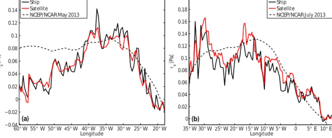
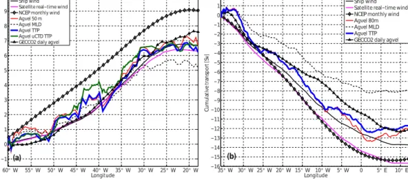
Overall, the satellite wind stress agrees well with the ship wind stress (Fig. 5) except in the region between 40 and 30^◦W at 14.5^◦N, where the zonal ship wind stress is larger than the zonal satellite wind stress, and at 11^◦S the ship wind

stress is generally smaller than the satellite wind stress. Since the 10 m wind speeds from the ship and satellite are very close to each other at both sections (not shown), the difference in the wind stress may be due to the use of a different drag coefficient formulation (COARE 3 for the CMEMS wind product; Large and Yeager, 2004, for ship wind stress).

In comparison to the NCAR/NCEP monthly zonal wind stress, the weaker ship wind stress in the western half of the 14.5^◦N section indicates that the cruise started with anomalously weak winds, while at 11^◦S the observed wind stress (both ship and satellite observation) was consistent with the monthly mean wind stress. It is also reported that differences in the different wind stress data may also arise from the unresolved local effect by the satellites and NCEP data (Mason et al., 2011; Pérez-Hernández et al., 2015). For instance, near the Canary Islands, the NCEP monthly data do not resolve the Von Karman structure caused by the interaction of wind with the islands due to its low resolution.

As expected, at 14.5^◦N, the indirect estimate of the Ek- man transport from the in situ wind stress is 6.7±3.5 Sv, only 0.4 Sv larger than that from the satellite wind stress. Us- ing the monthly mean wind stress from NCEP/NCAR during the M96/M97 cruise month (May 2013), the total transport is 8.8±1.4 Sv. The difference between the monthly wind estimate and in situ wind estimate is mainly due to the anomalously weak wind when the cruise started from the western boundary (Fig. 5a). At 11^◦S, the indirect Ekman transport from the in situ wind stress is 13.6±3.3 Sv, while the transport from the satellite wind stress is 2.0 Sv higher, due to the higher value of the satellite wind stress (Fig. 5b). The NCEP/NCAR monthly wind stress in July 2013 returns a transport of 15.1±1.9 Sv. The errors shown with the indirect ship wind estimates are given by the standard deviation of the long-term Ekman transport calculated using 6 h NCEP/CFSR wind stress between the years 2000 and 2011 at the two lat- itudes. The errors of the monthly estimates are given by the standard deviation of the monthly mean Ekman transport in May (July) between 1979 and 2013 at 14.5^◦N (11^◦S) calculated from the NCEP/NCAR monthly wind stress. Another source of uncertainty may arise from the wind stress calculation using different bulk formulas, which could lead to an uncertainty as large as 20 % (Large and Pond, 1981). This may explain the difference in the indirect estimates between using the in situ wind stress and the satellite wind stress at 11^◦S.

4.3.2 Direct method

The direct meridional Ekman transport is derived from vertically integrating the ageostrophic velocity profiles (Eq. 1, right-hand side). As already mentioned, one critical assumption is the integration depth (D_E). Applying the TTP as an estimate of D_E, the total Ekman transport at 14.5^◦N based on CTD data is 6.2±2.3 Sv, while applying a uniform depth of 50 m results in an alternative estimate of