Poleward Shift of the Major Ocean Gyres Detected in a Warming Climate
Hu Yang1 , Gerrit Lohmann1 , Uta Krebs-Kanzow1 , Monica Ionita1 , Xiaoxu Shi1 , Dimitry Sidorenko1 , Xun Gong1 , Xueen Chen2 , and Evan J. Gowan1
1Climate Sciences, Alfred Wegener Institute, Helmholtz Centre for Polar and Marine Research, Bremerhaven, Germany,2College of Oceanic and Atmospheric Sciences, Ocean University of China, Qingdao, China
Abstract
Recent evidence shows that wind-driven ocean currents, like the western boundary currents, are strongly affected by global warming. However, due to insufficient observations both on temporal and spatial scales, the impact of climate change on large-scale ocean gyres is still not clear. Here, based on satellite observations of sea surface height and sea surface temperature, we find a consistent poleward shift of the major ocean gyres. Due to strong natural variability, most of the observed ocean gyre shifts are not statistically significant, implying that natural variations may contribute to the observed trends. However, climate model simulations forced with increasing greenhouse gases suggest that the observed shift is most likely to be a response of global warming. The displacement of ocean gyres, which is coupled with the poleward shift of extratropical atmospheric circulation, has broad impacts on ocean heat transport, regional sea level rise, and coastal ocean circulation.Plain Language Summary
Ocean circulation plays a vital role in regulating the weather and climate and supporting marine life. Therefore, it is important to understand whether and how it responds to global warming. However, the available observations are currently sparse and short in duration, making it difficult to track the dynamic changes of large-scale ocean circulation. Here, we show for the first time, independent satellite observational evidence demonstrating that the large-scale ocean gyres are moving poleward during the past four decades. Further analysis based on climate models and various other data sets reveal that the poleward shifting of the ocean gyre circulation is most likely to be a consequence of global warming, which so far has not been well recognized by the public and the scientific community.1. Introduction
Ocean gyres represent large systems of ocean currents, which are driven by the wind (Munk, 1950). At the western edge of subtropical gyres are the western boundary currents, which carry warm water from the tropics poleward, contributing to a warm and wet climate on the adjacent mainland. The eastern margins of the subtropical gyres are manifested by upwelling and cold eastern boundary currents. These provide abundant nutrients for marine ecosystems and contribute to maintaining a relatively cold and dry climate on the nearby continents. Due to strong stratification, oceanic productivity is particularly low over the central parts of the subtropical gyres (commonly called ocean deserts), whereas the subpolar gyres are relatively nutrient rich, sustaining an abundance of marine life. Given the broad impacts of ocean gyres on the climate and ecosystems, it is crucial to understand how they respond to climate change.
In the past few decades, multiple lines of evidence indicate that the large-scale extratropical atmospheric circulation is shifting toward poles under global warming. This evidence includes poleward shifts of west- erly winds (Chen et al., 2008), jet streams (Archer & Caldeira, 2008), storm tracks (Yin, 2005), clouds (Norris et al., 2016), and the pattern of precipitation (Scheff & Frierson, 2012). Comparatively, large-scale ocean circulation changes due to global warming is largely uncertain, mostly due to insufficient ocean observations.
As ocean observations are restricted by short duration and sparse coverage, previous research mainly focused on the variability of ocean circulation from a regional perspective (Foukal & Lozier, 2017; Roemmich et al., 2007, 2016; Wu et al., 2012; Yang, Lohmann, et al., 2016). For example, Frankignoul et al. (2001) showed that the position of the Gulf Stream, derived from satellite altimetry in the 1990s, is 50–100 km north of
RESEARCH LETTER
10.1029/2019GL085868
Key Points:
• Satellite observations show a consistent poleward shift of the major ocean gyres during the past four decades
• Due to strong natural variability, most of the observed ocean gyre shifts are not statistically significant
• Climate model simulations suggest that the observed shift is most likely to be a response to global warming
Supporting Information:
• Supporting Information S1
• Text S1
Correspondence to:
H. Yang and G. Lohmann, hyang@awi.de;
gerrit.lohmann@awi.de
Citation:
Yang, H., Lohmann, G.,
Krebs-Kanzow, U., Ionita, M., Shi, X., Sidorenko, D., et al. (2020). Poleward shift of the major ocean gyres detected in a warming climate.Geophysical Research Letters,47, e2019GL085868.
https://doi.org/10.1029/2019GL085868
Received 17 OCT 2019 Accepted 3 JAN 2020
©2020. The Authors.
This is an open access article under the terms of the Creative Commons Attribution License, which permits use, distribution and reproduction in any medium, provided the original work is properly cited.
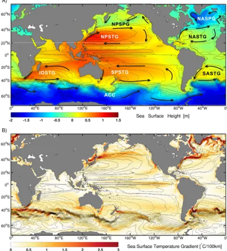
Figure 1.The major ocean gyres and associated climatological conditions. Contour lines represent the barotropic stream function. Solid lines indicate clockwise flow, and dashed lines indicate anticlockwise flow. (a) Background shading shows the sea surface height (SSH). Black arrows illustrate the significant features of the currents.
(b) Background shading represents the horizontal sea surface temperature gradient. Results are based on the last 100 years of the AWI-CM pre-industrial control run. The abbreviations in the figure are listed as follows: North Atlantic Subtropical Gyre (NASTG), South Atlantic Subtropical Gyre (SASTG), North Pacific Subtropical Gyre (NPSTG), South Pacific Subtropical Gyre (SPSTG), Indian Ocean Subtropical Gyre (IOSTG), North Pacific Subpolar Gyres (NPSPG), North Atlantic Subpolar Gyres (NASPG), and Antarctic Circumpolar Current (ACC).
the position estimated from expendable bathythermographs (XBT) during 1954–1998. A southward advance of the Eastern Australian Current (Ridgway, 2007), the Brazil Current front (Goni et al., 2011), and the Antarctic Circumpolar Current front (Sokolov & Rintoul, 2009) has been observed over the Southern Hemi- sphere. Roemmich et al. (2007, 2016) reported a strengthening of the South Pacific Subtropical Gyre, while Häkkinen and Rhines (2004) and Foukal and Lozier (2017) observed a weakening of the North Atlantic Subpolar Gyre since 1992.
Considering that direct continuous observations of ocean currents are rare, an indirect approach must be adopted to investigate the dynamic changes of large-scale ocean gyres. Under the constraint of geostrophic balance, the Coriolis force induced by ocean flow is balanced by the pressure gradient caused by the differ- ence in sea surface height (SSH). Thus, the centers of the anticyclonic subtropical gyres are characterized by relatively high regional SSH. The centers of the cyclonic subpolar gyres and the Antarctic Circumpo- lar Current are distinguished by relatively low regional SSH (Munk, 1950). Therefore, the SSH “hills” and
“valleys” can be used to locate the position of the ocean gyres (Figure 1a). Moreover, the subtropical gyres represent a circulation of warm water, while the subpolar water is relatively cold. The confluence of the warm subtropical gyres and the cold subpolar gyres generates sharp sea surface temperature (SST) fronts at the midlatitudes, namely, the subtropical fronts. These fronts mark the boundary between the subtropical and subpolar gyres (Figure 1b).
Geophysical Research Letters
10.1029/2019GL085868Figure 2.Schematic of the method of tracking the meridional variations of ocean gyres. As gyre-related SSH patterns, subtropical fronts, and barotropic stream function all resemble the shapes of hills. We use the center of mass of these hills to track the position of ocean gyres. The gray shading box illustrates the region (also shown as gray rectangles in Figures 3a and 4a) where the integration is performed. These regions are defined primarily based on the climatology position of each parameter and do not vary over time. Following equation (1),latis the latitudinal coordinate of each parameter. For the SSH parameter,ΔvarrepresentsSSH−SSHminfor calculating the position of subtropical gyres, andSSH−SSHmaxfor calculating the position of subpolar gyres.SSHminandSSHmaxare the regional minimum and maximum SSH within the integrated regions. For the SST parameter,Δvarrepresents horizontal SST gradient. For the stream function parameter,Δvarrepresents barotropic stream function.
Satellite altimetry has continuously monitored SSH since late 1992.
Satellite-based SST records have been collected for almost four decades, starting from the early 1980s. These data are independently observed and provide an unprecedented opportunity to explore the dynamic changes of the large-scale ocean gyres. In the present study, we evaluate the results from both satellite observations and climate simulations and find a consistent poleward shift of the major ocean gyres in a warming climate.
2. Data and Methods
2.1. Data and Simulations
Satellite-based SSH (data from 1992–2018 AVISO) and SST (data from 1982–2018 National Oceanic and Atmospheric Administration Optimum Interpolation Sea Surface Temperature, OISST) are used to investigate the dynamic changes of ocean gyres. Near-surface wind and sea level pres- sure data from the National Centers for Atmospheric Prediction/National Center for Atmospheric Research (NCEP/NCAR, Kalnay et al., 1996), National Centers for Atmospheric Prediction-Department of Energy (NCEP/DOE, Kanamitsu et al., 2002), and ERA-Interim reanalysis data sets are included to explore the dynamic mechanism responsible for the ocean circulation changes.
To validate the observational trend, two series of simulations, namely, a pre-industrial control run and a set of doubled CO2runs, are conducted by the Alfred Wegener Institute Climate Model (AWI-CM) using the same configuration as in Sidorenko et al. (2015). The pre-industrial control run is integrated for 800 years, forced by greenhouse gas concentrations fixed at the 1850 levels. The doubled CO2runs are integrated for 150 years by linearly increasing the concentration of greenhouse gases to a doubled level. The doubled CO2runs are performed five times starting from different initial conditions obtained from the pre-industrial control run.
To reduce the amplitude of natural climate variability, the ensemble mean of the last 10 years of the doubled CO2simulations are then used to compare with the last 100 years of the pre-industrial control run.
Furthermore, to demonstrate that the results are not model dependent, thepiControland 1pctCO2simu- lations from the fifth phase of the Coupled Model Intercomparison Project (CMIP5) (Taylor et al., 2012) are presented as well in the supporting information. Twenty-two climate models are included to obtain an ensemble trend. Detailed information on the models used in this study is summarized in Table S1.
2.2. Methods
As mentioned in section 1, the gyre center and gyre boundary are physically associated with the patterns of SSH and SST gradient (Figure 1). To examine the meridional variations of ocean gyres, we introduce two indices based on these two parameters. Imagine that gyre-related SSH patterns resemble shape of “hills” (the subpolar SSH “valleys” can be mirrored into “hills” by subtracting the regional maximum SSH), we use the
“center of mass” of these “hills” to identify their position. The detailed computation follows the equation below:
P=∫ Δvar·lat
∫ Δvar (1)
wherePis the meridional location of ocean gyres andlatis the latitudinal coordinate of SSH.Δvarrepresents SSH−SSHminfor calculating the position of subtropical gyres, andSSH−SSHmaxfor calculating the position of subpolar gyres (Figure 2). TheSSHminandSSHmaxdenote the regional minimum and maximum SSH within the integrated regions (as shown by gray rectangles in Figure 3a). These regions are defined primarily based on the climatology position of the gyre center. They do not vary over time.
In a similar way, the meridional variations of gyre boundaries are also estimated based on the SST gradients.
Following equation (1), here,Δvardenotes the horizontal SST gradient (includes both zonal and meridional components). The integrated regions are given by the gray rectangles in Figure 4a, following the climatology positions of the subtropical fronts.
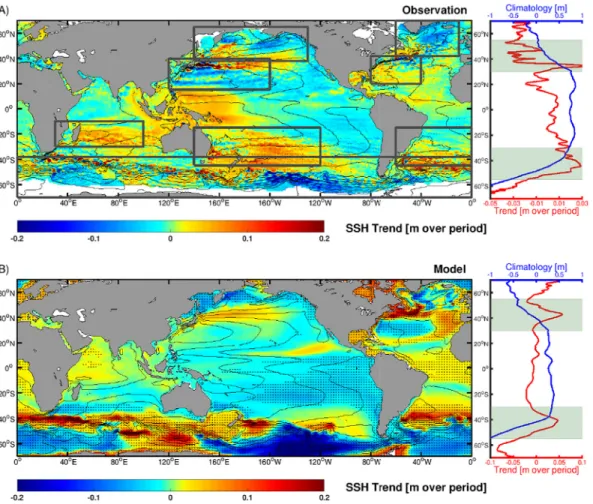
Figure 3.Observational (a) and modeled (b) trends (shading) and climatology (contours) of SSH. (a) Trends of SSH based on satellite altimetry (1993–2018). The globally averaged sea level rise (8 cm) has been subtracted. Stippling indicates regions where the trends pass the 95% confidence level (Student'sttest). (b) Ensemble SSH change in the doubled CO2simulations relative to the pre-industrial control simulation carried out by AWI-CM. Stippling indicates areas where the magnitude of the trend is larger than the standard deviation of the local variability. The subpanel at the right side of each graph shows the zonally averaged trend (red) and climatology (blue) of SSH, with the subtropical zone highlighted in gray.
To check whether our indices derived from SSH and SST gradients are suitable to locate the ocean gyres, we verified them in our climate model. The results suggest that they are excellent proxies to reconstruct the position of ocean gyres (see section “Validation of metrics of ocean gyres position” in the supporting information).
In the climate model, the meridional positions of the ocean gyres are also estimated following equation (1), whereΔvardenotes the barotropic stream function. Here, the integration is performed within the boundary (zero crossing of barotropic stream function) of ocean gyres at each ocean basin. This is different from the approach applied in the observations, in which the integration is performed within the predefined regions, because it is hard to find a common threshold to identify the boundary of the ocean gyres in the observations.
3. Poleward Shift of the Major Ocean Gyres
3.1. Observational Results
Figures 3a and 4a present the linear trends (shading) of SSH and SST gradients during the satellite era.
Enhanced regional sea level rise is found over the midlatitude bands in both hemispheres, while the sea level rise over the high latitudes is below the globally averaged trend. Comparing the trend of SSH with its climatology pattern (contours), the enhanced sea level rise over the midlatitudes illustrates that the subtrop- ical SSH “hills” and subpolar SSH “valleys” have shifted toward the poles. Associated with the SSH trend,
Geophysical Research Letters
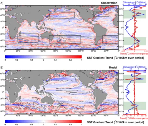
10.1029/2019GL085868Figure 4.Observational (a) and modeled (b) trends (shading) and climatology (contours) of the sea surface
temperature gradients. Contours give the SST gradients at level of 0.5◦C/100 km. (a) Observational trends based on the NOAA Optimum Interpolation Sea Surface Temperature data set covering 1982–2018. Stippling indicates regions where the trends pass the 95% confidence level (Student'sttest). (b) Trend in the doubled CO2simulations relative to the pre-industrial control simulation carried out by AWI-CM. Stippling indicates areas where the magnitude of the trend is larger than the standard deviation of the local variability. The subpanel at the right side of each figure shows the zonally averaged trend (red) and climatology (blue) of sea surface temperature gradients, with the subtropical zone highlighted in gray.
increasing/decreasing trends of SST gradients are found over polar/equator flanks of the subtropical fronts respectively, implying that the subtropical fronts have a similar signal of poleward displacement.
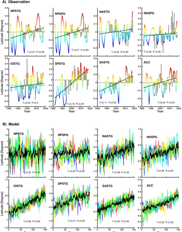
Figure 5a shows the interannual variations of the location of the major ocean gyres based on SSH and SST gradients. The time series of both metrics show similar temporal variations in the overlapping period (1993–2018). Moreover, positive trends are found for all the major ocean gyres, illustrating that they are con- sistently shifting toward the poles during the past four decades. The average magnitude of the shift is on the order of 0.07◦per decade. Most of the Southern Hemisphere ocean gyres (except the Indian Ocean Subtropi- cal Gyre) have experienced a statistically significant poleward shift, while the ocean gyre displacements over the Northern Hemisphere are not statistically significant. These trends are superimposed by strong natural variations. It remains unclear whether the poleward movements are due to natural climate variability or long-term anthropogenic climate change.
3.2. Climate Model Results
To address this issue, we compared the observational results with the results from the climate model (AWI-CM). As presented in Figures 3b and 4b, the ensemble simulations are consistent with the observa- tions showing an enhanced SSH increase over the midlatitudes. Similarly, there are positive/negative trends of the SST gradients over the polar/equator flanks of the subtropical fronts, respectively. Tracking the merid- ional position of ocean gyres in the doubled CO2simulations (Figure 5b) illustrates that all the major ocean gyres shift toward the poles. We notice that the North Pacific Subtropical Gyre and the North Pacific Subpolar Gyre have minor poleward shifts in comparison with their strong internal variability.
In addition to our results from AWI-CM, we also carry out a comprehensive analysis on model data from CMIP5 (Taylor et al., 2012). The ensemble results from the 1pctCO2experiment also show poleward
Figure 5.Observational (a) and modeled (b) time series of latitudinal variations of the major ocean gyres. (a) Gray bars are indices derived from the center of the regional high and low SSH based on the satellite altimetry record. Colored lines are estimations derived from the position of subtropical fronts based on the NOAA Optimum Interpolation Sea Surface Temperature data set. (b) Results from the 150 year AWI-CM doubled CO2simulations. The estimation is calculated based on the barotropic stream function weighted center of each gyre. Colored thin lines represent individual ensemble members. The thick black lines give the ensemble mean variations. The corresponding linear trends (T) are given by the text, in units of degrees per decade. A positive trend indicates a poleward shift.
The associatedpvalues (P) are also given based on the Student'sttest.
Geophysical Research Letters
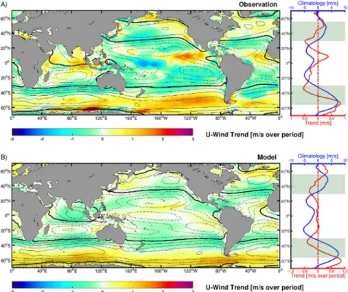
10.1029/2019GL085868Figure 6.Observational and modeled climatology (contours) and trends (shading) of the zonal component of the near ocean surface wind. (a) Ensemble trends of the zonal near ocean surface wind based on the NCEP/NCAR, NCEP/DOE and NERA-Interim reanalysis data sets covering 1979–2018. Stippling indicates regions where the trends pass the 95%
confidence level (Student'sttest). (b) Zonal near ocean surface wind change in the doubled CO2simulations relative to the pre-industrial control simulation carried out by AWI-CM. Stippling indicates areas where the magnitude of the trend is larger than the standard deviation of the local variability. The subpanel at the right side of each graph shows the zonally averaged climatology (blue) and trend (red) of zonal near ocean surface wind.
displacement of the ocean gyres (Figures S1 and S2). The agreement among these broad ranges of observa- tions and climate simulations suggests that poleward migration of the major ocean gyres is most likely to be a response to global warming.
4. Mechanism
According to the theory of ocean circulation, the ocean gyres are driven by near-surface ocean wind, more specifically the wind stress curl (Munk, 1950). To explore the mechanism driving the shift of ocean gyres, we examine the trends of near-surface wind and associated sea level pressure (Figure S3). As shown in Figure 6a, a large portion of subtropical oceans (approximately between 20–40◦latitude bands) show a change of veloc- ity of the easterly winds, while there is a change of velocity of the westerly winds over the 40–60◦latitude bands. Compared with the climatological (contours) pattern of zonal wind, the observational wind pattern change implies that the extratropical atmospheric surface winds have shifted toward higher latitudes during the past four decades. Consequently, the wind stress curl has shifted as well (not shown). In agreement with observations, the ensemble climate model result (Figure 6b) displays a similar pattern of shifting wind under forcing of increasing CO2. We propose that the movement of the near-surface wind drives the displacement of the ocean gyres.
A large number of climate simulations have demonstrated that the extratropical atmospheric circulation undergoes a systematic poleward shift under greenhouse gases forcing (Cai, 2006; Cai et al., 2003; Fyfe &
Saenko, 2006; Fyfe et al., 1999; Kushner et al., 2001; Saenko et al., 2005; Sen Gupta et al., 2009). On one hand, the displacement of the atmospheric circulation can drive the shift in ocean gyres. On the other hand, shifting ocean gyres contribute to moving the subtropical front, which may also alter the atmospheric circu- lation (Hudson, 2012; Nakamura et al., 2004). Thus, these dynamics are strongly coupled. We believe that the
identified shift in ocean gyres is another manifestation of a systematic movement of the entire extratropical climate zone.
5. Discussion and Conclusions
Based on results from satellite observations and climate simulations, we identify a consistent poleward shift of the major ocean gyres in a warming climate. Due to short temporal coverage and strong natural cli- mate variability, most of the observed shifts are not statistically significant, especially over the Northern Hemisphere. However, model simulations suggest that poleward shift of ocean gyres are most likely to be a consequence of global warming, driven by a systematic poleward displacement of the extratropical atmospheric circulation.
The displacement of extratropical atmospheric circulation has been explored intensively in the past two decades. Investigations have pointed out that two phenomena are related to such a displacement, that is, pos- itive trends of annular modes (Fyfe et al., 1999; Thompson et al., 2000) and expanding tropics (Seidel et al., 2008). Model simulations imply that increasing greenhouse gases (Cai et al., 2003; Fyfe et al., 1999; Kushner et al., 2001), ozone depletion over the South Pole (Thompson & Solomon, 2002; Thompson et al., 2011) and increasing aerosols (Allen et al., 2012) over the Northern Hemisphere all contribute to the observed shift in atmospheric circulation, suggesting that human activity is reshaping the climate. However, more recent studies highlighted that the observed climate change is still within the magnitude of natural climate vari- ability (Allen & Kovilakam, 2017; Garfinkel et al., 2015; Grise et al., 2019; Waugh et al., 2018). For example, in the satellite altimetry record, there is an equatorward shift of the North Atlantic Subtropical Gyre from the 1990s to the 2000s (Figure 5a), which conflicts with our model simulations. This is because the North Atlantic Oscillation, which regulates the position of the North Atlantic Subtropical Gyre (Frankignoul et al., 2001; Joyce et al., 2000), has shifted to a negative phase during 1990–2010. Nevertheless, from a long-term perspective, our SST-based metric and many other studies have demonstrated that the Gulf Stream (or North Atlantic Subtropical Gyre) has experienced an overall northward displacement during the twentieth century (Frankignoul et al., 2001; Yin & Goddard, 2013), which is in line with the model results.
Regarding the rate of the shift, our estimation of the shift of subtropical/subpolar gyres is on the order of 0.1/0.04◦per decade during the past four decades. The estimated rate for tropical expansion is on the order of 0.2–3.0◦per decade, depending on the data sets and methods of analysis (Davis & Rosenlof, 2012). Recent work suggested that the rate of tropical expansion is most likely on the order of 0.2◦per decade, which is consistent with our estimation of the movement of subtropical gyres (Paul et al., 2018; Waugh et al., 2018).
Marine sediment records illustrate that the Agulhas Current was 7◦equatorward of its modern position (Bard & Rickaby, 2009) during the glacial period. This implies that the ocean circulation may have shifted significantly since the Last Glacial Maximum (21 ka before present). Considering that the present climate is already relatively warm compared to the last glacial period, the space for ocean gyres to shift in the future may be limited. However, uncertainty also exists in our estimation of the magnitude of the shift due to short term natural climate variability. Since the period of satellite observations is still relatively short, it may take some time before the signal of global warming overcomes natural variability and a robust measurement can be achieved. The proxy record from the Agulhas Current (Bard & Rickaby, 2009) provides a good analogue for detecting the past limit of a circulation shift. We propose that long-term observations combined with more paleoclimate records, in particular, over some key regions, such as western boundary currents and the subtropical fronts, will provide a more accurate estimation on how fast and how much the climate zone can shift.
The poleward shift of the major ocean gyres may have broad environmental and societal impacts. There is evidence showing that the western boundary currents are transporting more heat to the midlatitudes (Yang, Liu, et al., 2016; Yang, Lohmann, et al., 2016). Yin (2005) demonstrated that there is a consistent poleward movement of storm tracks and the jet stream, most likely associated with the change in the subtropical front induced by ocean gyre movement (Primeau & Cessi, 2001). The eastern boundary of the subtropical gyres, such as the Benguela ecosystem, has also been shrinking over the past three decades (Blamey et al., 2015).
The margins of the gyres experience the most significant changes. For example, the Gulf of Maine, located at the north flank of the Gulf Stream, is undergoing vigorous ocean temperature increases even though the Gulf Stream is observed to be weaker (Caesar et al., 2018; Dima & Lohmann, 2010). Such changes have had disastrous consequences for the local cod fishery (Pershing et al., 2015). Similar impacts have also been
Geophysical Research Letters
10.1029/2019GL085868reported for the Uruguayan and Argentinean industrial fisheries due to enhanced warming at the margins of Southern Atlantic Subtropical Gyre (Auad & Martos, 2012; Ignacio et al., 2019). The shift in ocean gyres generates a pronounced sea level rise band over the midlatitudes (Figure 3) (Yin & Goddard, 2013). This pattern is superimposed on global mean sea level rise, causing an additional threat to the nearby islands and the mainland in the midlatitudes, for instance, the northeast coast of North America (Yin & Goddard, 2013). The ocean desert is expanding and causing a reduction of total marine productivity (Steinacher et al., 2010; Stramma et al., 2008). Previously, the mechanism was explained by a stronger stratification induced by surface warming (Stramma et al., 2008). Our study reveals that the displacement of the subtropical gyre may be expanding the ocean desert as well. As part of global circulation, the shifting large-scale ocean gyres has the potential to reshape ocean circulation over the tropics, near coastal regions, and also change merid- ional overturning circulation (Lique & Thomas, 2018). However, to our knowledge, these topics remain poorly studied.
References
Allen, R. J., & Kovilakam, M. (2017). The role of natural climate variability in recent tropical expansion.Journal of Climate,30(16), 6329–6350.
Allen, R. J., Sherwood, S. C., Norris, J. R., & Zender, C. S. (2012). Recent Northern Hemisphere tropical expansion primarily driven by black carbon and tropospheric ozone.Nature,485(7398), 350.
Archer, C. L., & Caldeira, K. (2008). Historical trends in the jet streams.Geophysical Research Letters,35, L08803. https://doi.org/10.1029/
2008GL033614
Auad, G., & Martos, P. (2012). Climate variability of the northern Argentinean shelf circulation: Impact on Engraulis anchoita.The International Journal of Ocean and Climate Systems,3(1), 17–43.
Bard, E., & Rickaby, R. E. (2009). Migration of the subtropical front as a modulator of glacial climate.Nature,460(7253), 380.
Blamey, L. K., Shannon, L. J., Bolton, J. J., Crawford, R. J., Dufois, F., Evers-King, H., et al. (2015). Ecosystem change in the southern Benguela and the underlying processes.Journal of Marine Systems,144, 9–29.
Caesar, L., Rahmstorf, S., Robinson, A., Feulner, G., & Saba, V. (2018). Observed fingerprint of a weakening Atlantic Ocean overturning circulation.Nature,556(7700), 191.
Cai, W. (2006). Antarctic ozone depletion causes an intensification of the Southern Ocean super-gyre circulation.Geophysical Research Letters,33, L03712. https://doi.org/10.1029/2005GL024911
Cai, W., Whetton, P. H., & Karoly, D. J. (2003). The response of the Antarctic Oscillation to increasing and stabilized atmospheric CO2. Journal of Climate,16(10), 1525–1538.
Chen, G., Lu, J., & Frierson, D. M. (2008). Phase speed spectra and the latitude of surface westerlies: Interannual variability and global warming trend.Journal of Climate,21(22), 5942–5959.
Davis, S. M., & Rosenlof, K. H. (2012). A multidiagnostic intercomparison of tropical-width time series using reanalyses and satellite observations.Journal of Climate,25(4), 1061–1078.
Dima, M., & Lohmann, G. (2010). Evidence for two distinct modes of large-scale ocean circulation changes over the last century.Journal of Climate,23(1), 5–16.
Foukal, N. P., & Lozier, M. S. (2017). Assessing variability in the size and strength of the North Atlantic subpolar gyre.Journal of Geophysical Research: Oceans,122, 6295–6308. https://doi.org/10.1002/2017JC012798
Frankignoul, C., de Coëtlogon, G., Joyce, T. M., & Dong, S. (2001). Gulf Stream variability and ocean–atmosphere interactions.Journal of physical Oceanography,31(12), 3516–3529.
Fyfe, J., Boer, G., & Flato, G. (1999). The Arctic and Antarctic Oscillations and their projected changes under global warming.Geophysical Research Letters,26(11), 1601–1604.
Fyfe, J. C., & Saenko, O. A. (2006). Simulated changes in the extratropical Southern Hemisphere winds and currents.Geophysical Research Letters,33, L06701. https://doi.org/10.1029/2005GL025332
Garfinkel, C. I., Waugh, D. W., & Polvani, L. M. (2015). Recent Hadley cell expansion: The role of internal atmospheric variability in reconciling modeled and observed trends.Geophysical Research Letters,42, 10,824–10,831. https://doi.org/10.1002/2015GL066942 Goni, G. J., Bringas, F., & DiNezio, P. N. (2011). Observed low frequency variability of the Brazil Current front.Journal of Geophysical
Research,116, C10037. https://doi.org/10.1029/2011JC007198
Grise, K. M., Davis, S. M., Simpson, I. R., Waugh, D. W., Fu, Q., Allen, R. J., et al. (2019). Recent tropical expansion: Natural variability or forced response?Journal of Climate,32(5), 1551–1571.
Häkkinen, S., & Rhines, P. B. (2004). Decline of subpolar North Atlantic circulation during the 1990s.Science,304(5670), 555–559.
Hudson, R. (2012). Measurements of the movement of the jet streams at mid-latitudes, in the Northern and Southern Hemispheres, 1979 to 2010.Atmospheric Chemistry and Physics,12(16), 7797–7808.
Ignacio, G., Leonardo, O., Yamandú, M., Alberto, R. P., & Omar, D. (2019). Evidence of ocean warming in Uruguay's fisheries landings:
The mean temperature of the catch approach.Marine Ecology Progress Series,625, 115–125.
Joyce, T. M., Deser, C., & Spall, M. A. (2000). The relation between decadal variability of subtropical mode water and the North Atlantic Oscillation.Journal of Climate,13(14), 2550–2569.
Kalnay, E., Kanamitsu, M., Kistler, R., Collins, W., Deaven, D., Gandin, L., et al. (1996). The NCEP/NCAR 40-year reanalysis project.
Bulletin of the American meteorological Society,77(3), 437–471.
Kanamitsu, M., Ebisuzaki, W., Woollen, J., Yang, S.-K., Hnilo, J., Fiorino, M., & Potter, G. (2002). NCEP-DOE AMIP-II Reanalysis (R-2).
Bulletin of the American Meteorological Society,83(11), 1631–1643.
Kushner, P. J., Held, I. M., & Delworth, T. L. (2001). Southern Hemisphere atmospheric circulation response to global warming.Journal of Climate,14(10), 2238–2249.
Lique, C., & Thomas, M. D. (2018). Latitudinal shift of the Atlantic Meridional Overturning Circulation source regions under a warming climate.Nature Climate Change,8(11), 1013.
Munk, W. H. (1950). On the wind-driven ocean circulation.Journal of meteorology,7(2), 80–93.
Acknowledgments
We thank Gregor Knorr for providing an internal review of this manuscript, and Qiang Wang for clarifying the calculation of dynamic and steric sea level in the AWI-CM. We would also like to acknowledge Nicholas Foukal and another anonymous reviewer for providing constructive comments. This work was supported through DFG SPP-1889 “Sea-level change and society” project SLOSH (KR4478/1-1).
Furthermore, thanks to the projects PACMEDY and PalMOD funded through BMBF and the open fund of State Key Laboratory of Loess and Quaternary Geology, Institute of Earth Environment, CAS (SKLLQG1920).
The altimeter products were produced by Ssalto/Duacs and distributed by Aviso, with support from Cnes (http://
www.aviso.altimetry.fr/duacs/). The sea surface temperature data (NOAA_OI_SST_V2) are provided by the NOAA/OAR/ESRL PSD, Boulder, Colorado, USA, from their website (https://www.esrl.noaa.gov/psd/). We acknowledge the World Climate Research Programme's Working Group on Coupled Modelling, which is responsible for CMIP5, and we thank the climate modeling groups (listed in Table S1 of this paper) for producing and making available their model output. For CMIP, the U.S. Department of Energy's Program for Climate Model Diagnosis and Intercomparison provides coordinating support and led development of software infrastructure in partnership with the Global Organization for Earth System Science Portals.
Nakamura, H., Sampe, T., Tanimoto, Y., & Shimpo, A. (2004). Observed associations among storm tracks, jet streams and midlatitude oceanic fronts.Earths Climate: The Ocean–Atmosphere Interaction, Geophys. Monogr,147, 329–345.
Norris, J. R., Allen, R. J., Evan, A. T., Zelinka, M. D., O'Dell, C. W., & Klein, S. A. (2016). Evidence for climate change in the satellite cloud record.Nature,536(7614), 72–75.
Paul, W. S., Jian, L., Kevin, M. G., Sean, M. D., & Thomas, B. (2018). Re-examining tropical expansion.Nature Climate Change,8, 768–775.
Pershing, A. J., Alexander, M. A., Hernandez, C. M., Kerr, L. A., Le Bris, A., Mills, K. E., et al. (2015). Slow adaptation in the face of rapid warming leads to collapse of the Gulf of Maine cod fishery.Science,350(6262), 809–812.
Primeau, F., & Cessi, P. (2001). Coupling between wind-driven currents and midlatitude storm tracks.Journal of climate,14(6), 1243–1261.
Ridgway, K. (2007). Long-term trend and decadal variability of the southward penetration of the East Australian Current.Geophysical Research Letters,34, L13613. https://doi.org/10.1029/2007GL030393
Roemmich, D., Gilson, J., Davis, R., Sutton, P., Wijffels, S., & Riser, S. (2007). Decadal spinup of the South Pacific subtropical gyre.Journal of Physical Oceanography,37(2), 162–173.
Roemmich, D., Gilson, J., Sutton, P., & Zilberman, N. (2016). Multidecadal change of the South Pacific gyre circulation.Journal of Physical Oceanography,46(6), 1871–1883.
Saenko, O. A., Fyfe, J. C., & England, M. H. (2005). On the response of the oceanic wind-driven circulation to atmospheric CO2increase.
Climate Dynamics,25(4), 415–426.
Scheff, J., & Frierson, D. (2012). Twenty-first-century multimodel subtropical precipitation declines are mostly midlatitude shifts.Journal of Climate,25(12), 4330–4347.
Seidel, D. J., Fu, Q., Randel, W. J., & Reichler, T. J. (2008). Widening of the tropical belt in a changing climate.Nature geoscience,1(1), 21–24.
Sen Gupta, A., Santoso, A., Taschetto, A. S., Ummenhofer, C. C., Trevena, J., & England, M. H. (2009). Projected changes to the Southern Hemisphere ocean and sea ice in the IPCC AR4 climate models.Journal of Climate,22(11), 3047–3078.
Sidorenko, D., Rackow, T., Jung, T., Semmler, T., Barbi, D., Danilov, S., et al. (2015). Towards multi-resolution global climate modeling with ECHAM6-FESOM. Part I: Model formulation and mean climate.Climate Dynamics,44(3-4), 757–780.
Sokolov, S., & Rintoul, S. R. (2009). Circumpolar structure and distribution of the Antarctic Circumpolar Current fronts: 2. Variability and relationship to sea surface height.Journal of Geophysical Research,114, C11019. https://doi.org/10.1029/2008JC005248
Steinacher, M., Joos, F., Frölicher, T., Bopp, L., Cadule, P., Cocco, V., et al. (2010). Projected 21st century decrease in marine productivity:
A multi-model analysis.Biogeosciences,7(3), 979–1005.
Stramma, L., Johnson, G. C., Sprintall, J., & Mohrholz, V. (2008). Expanding oxygen-minimum zones in the tropical oceans.science, 320(5876), 655–658.
Taylor, K. E., Stouffer, R. J., & Meehl, G. A. (2012). An overview of CMIP5 and the experiment design.Bulletin of the American Meteorological Society,93(4), 485–498.
Thompson, D. W., & Solomon, S. (2002). Interpretation of recent Southern Hemisphere climate change.Science,296(5569), 895–899.
Thompson, D. W., Solomon, S., Kushner, P. J., England, M. H., Grise, K. M., & Karoly, D. J. (2011). Signatures of the Antarctic ozone hole in Southern Hemisphere surface climate change.Nature Geoscience,4(11), 741.
Thompson, D. W., Wallace, J. M., & Hegerl, G. C. (2000). Annular modes in the extratropical circulation. Part II: Trends.Journal of climate, 13(5), 1018–1036.
Waugh, D. W., Grise, K. M., Seviour, W. J., Davis, S. M., Davis, N., Adam, O., et al. (2018). Revisiting the relationship among metrics of tropical expansion.Journal of Climate,31(18), 7565–7581.
Wu, L., Cai, W., Zhang, L., Nakamura, H., Timmermann, A., Joyce, T., et al. (2012). Enhanced warming over the global subtropical western boundary currents.Nature Climate Change,2(3), 161–166.
Yang, H., Liu, J., Lohmann, G., Shi, X., Hu, Y., & Chen, X. (2016). Ocean-atmosphere dynamics changes associated with prominent ocean surface turbulent heat fluxes trends during 1958–2013.Ocean Dynamics,66(3), 353–365.
Yang, H., Lohmann, G., Wei, W., Dima, M., Ionita, M., & Liu, J. (2016). Intensification and poleward shift of subtropical western boundary currents in a warming climate.Journal of Geophysical Research: Oceans,121, 4928–4945. https://doi.org/10.1002/2015JC011513 Yin, J. (2005). A consistent poleward shift of the storm tracks in simulations of 21st century climate.Geophysical Research Letters,32,
L18701. https://doi.org/10.1029/2005GL023684
Yin, J., & Goddard, P. B. (2013). Oceanic control of sea level rise patterns along the East Coast of the United States.Geophysical Research Letters,40, 5514–5520. https://doi.org/10.1002/2013GL057992