www.biogeosciences.net/13/4595/2016/
doi:10.5194/bg-13-4595-2016
© Author(s) 2016. CC Attribution 3.0 License.
Effect of ocean acidification and elevated f CO 2 on trace gas production by a Baltic Sea summer phytoplankton community
Alison L. Webb1,2, Emma Leedham-Elvidge1, Claire Hughes3, Frances E. Hopkins4, Gill Malin1, Lennart T. Bach5, Kai Schulz6, Kate Crawfurd7, Corina P. D. Brussaard7,8, Annegret Stuhr5, Ulf Riebesell5, and Peter S. Liss1
1Centre for Ocean and Atmospheric Sciences, School of Environmental Science, University of East Anglia, Norwich, NR4 7TJ, UK
2Groningen Institute for Evolutionary Life Sciences, University of Groningen, 9700 CC Groningen, the Netherlands
3Environmental Department, University of York, York, YO10 5DD, UK
4Plymouth Marine Laboratory, Plymouth, PL1 3DH, UK
5GEOMAR Helmholtz Centre for Ocean Research Kiel, Düsternbrooker Weg 20, 24148 Kiel, Germany
6Centre for Coastal Biogeochemistry, School of Environment, Science and Engineering, Southern Cross University, Lismore, NSW 2480, Australia
7Department of Biological Oceanography, NIOZ – Royal Netherlands Institute for Sea Research, P.O. Box 59, 1790 AB Den Burg, Texel, the Netherlands
8Aquatic Microbiology, Institute for Biodiversity and Ecosystem Dynamics, University of Amsterdam, P.O. Box 94248, 1090 GE Amsterdam, the Netherlands
Correspondence to:Alison L. Webb (a.l.webb@rug.nl)
Received: 6 November 2015 – Published in Biogeosciences Discuss.: 28 January 2016 Revised: 17 June 2016 – Accepted: 12 July 2016 – Published: 15 August 2016
Abstract. The Baltic Sea is a unique environment as the largest body of brackish water in the world. Acidification of the surface oceans due to absorption of anthropogenic CO2 emissions is an additional stressor facing the pelagic community of the already challenging Baltic Sea. To in- vestigate its impact on trace gas biogeochemistry, a large- scale mesocosm experiment was performed off Tvärminne Research Station, Finland, in summer 2012. During the sec- ond half of the experiment, dimethylsulfide (DMS) concen- trations in the highest-fCO2mesocosms (1075–1333 µatm) were 34 % lower than at ambient CO2(350 µatm). However, the net production (as measured by concentration change) of seven halocarbons analysed was not significantly affected by even the highest CO2levels after 5 weeks’ exposure. Methyl iodide (CH3I) and diiodomethane (CH2I2) showed 15 and 57 % increases in mean mesocosm concentration (3.8±0.6 increasing to 4.3±0.4 pmol L−1 and 87.4±14.9 increas- ing to 134.4±24.1 pmol L−1 respectively) during Phase II of the experiment, which were unrelated to CO2 and cor- responded to 30 % lower Chl a concentrations compared to Phase I. No other iodocarbons increased or showed
a peak, with mean chloroiodomethane (CH2ClI) concen- trations measured at 5.3 (±0.9) pmol L−1 and iodoethane (C2H5I) at 0.5 (±0.1) pmol L−1. Of the concentrations of bromoform (CHBr3; mean 88.1±13.2 pmol L−1), dibro- momethane (CH2Br2; mean 5.3±0.8 pmol L−1), and di- bromochloromethane (CHBr2Cl, mean 3.0±0.5 pmol L−1), only CH2Br2 showed a decrease of 17 % between Phases I and II, with CHBr3and CHBr2Cl showing similar mean con- centrations in both phases. Outside the mesocosms, an up- welling event was responsible for bringing colder, high-CO2, low-pH water to the surface starting on dayt16 of the ex- periment; this variable CO2system with frequent upwelling events implies that the community of the Baltic Sea is accli- mated to regular significant declines in pH caused by up to 800 µatmfCO2. After this upwelling, DMS concentrations declined, but halocarbon concentrations remained similar or increased compared to measurements prior to the change in conditions. Based on our findings, with future acidification of Baltic Sea waters, biogenic halocarbon emissions are likely to remain at similar values to today; however, emissions of biogenic sulfur could significantly decrease in this region.
4596 A. L. Webb et al.: Effect of ocean acidification and elevatedfCO2 1 Introduction
Anthropogenic activity has increased the fugacity of at- mospheric carbon dioxide (fCO2) from 280 µatm (pre- Industrial Revolution) to over 400 µatm today (Hartmann et al., 2013). The IPCC AR5 long-term projections for atmo- spheric pCO2 and associated changes to the climate have been established for a variety of scenarios of anthropogenic activity until the year 2300. As the largest global sink for at- mospheric CO2, the global ocean has absorbed an estimated 30 % of excess CO2produced (Canadell et al., 2007). With atmospheric pCO2 projected to possibly exceed 2000 µatm by the year 2300 (Collins et al., 2013; Cubasch et al., 2013), the ocean will take up increasing amounts of CO2, with a po- tential lowering of surface ocean pH by over 0.8 units (Raven et al., 2005). The overall effect of acidification on the bio- geochemistry of surface ocean ecosystems is unknown and currently unquantifiable, with a wide range of potential pos- itive and negative impacts (Doney et al., 2009; Hofmann et al., 2010; Ross et al., 2011).
A number of volatile organic compounds are produced by marine phytoplankton (Liss et al., 2014), including the cli- matically important trace gas dimethylsulfide (DMS, C2H6S) and a number of halogen-containing organic compounds (halocarbons), including methyl iodide (CH3I) and bromo- form (CHBr3). These trace gases are a source of sulfate par- ticles and halide radicals when oxidised in the atmosphere and have important roles as ozone catalysts in the tropo- sphere and stratosphere (O’Dowd et al., 2002; Solomon et al., 1994) and as cloud condensation nuclei (CCNs; Charl- son et al., 1987).
DMS is found globally in surface waters originating from the algal-produced precursor dimethylsulfoniopropi- onate (DMSP; C5H10O2S). Both DMS and DMSP provide the basis for major routes of sulfur and carbon flux through the marine microbial food web and can provide up to 100 % of the bacterial and phytoplanktonic sulfur demand (Simó et al., 2009; Vila-Costa et al., 2006a). DMS is also a volatile compound which readily passes through the marine bound- ary layer to the troposphere, where oxidation results in a number of sulfur-containing particles important for atmo- spheric climate feedbacks (Charlson et al., 1987; Quinn and Bates, 2011); for this reason, any change in the production of DMS may have significant implications for climate regula- tion. Several previous acidification experiments have shown differing responses of both compounds (e.g. Avgoustidi et al., 2012; Hopkins et al., 2010; Webb et al., 2015), while oth- ers have shown delayed or more rapid responses as a direct effect of CO2(e.g. Archer et al., 2013; Vogt et al., 2008). Fur- ther, some laboratory incubations of coastal microbial com- munities showed increased DMS production with increased fCO2(Hopkins and Archer, 2014) but lower DMSP produc- tion. The combined picture arising from existing studies is that the response of communities tofCO2perturbation is not predictable and requires further study. Previous studies mea-
suring DMS in the Baltic Sea measured concentrations up to 100 nmol L−1during the summer bloom, making the Baltic Sea a significant source of DMS (Orlikowska and Schulz- Bull, 2009).
In surface waters, halocarbons such as methyl io- dide (CH3I), chloroiodomethane (CH2ClI), and bromoform (CHBr3) are produced by biological and photochemical processes: many marine microbes (for example cyanobac- teria: Hughes et al., 2011; diatoms: Manley and De La Cuesta, 1997; and haptophytes: Scarratt and Moore, 1998) and macroalgae (e.g. brown-algalFucusspecies: Chance et al., 2009; red algae: Leedham et al., 2013) utilise halides from seawater and emit a range of organic and inorganic halogenated compounds. This production can lead to sig- nificant annual flux to the marine boundary layer in the or- der of 10 Tg iodine-containing compounds (“iodocarbons”;
O’Dowd et al., 2002) and 1 Tg bromine-containing com- pounds (“bromocarbons”; Goodwin et al., 1997) into the atmosphere. The effect of acidification on halocarbon con- centrations has received limited attention, but two acidifica- tion experiments measured lower concentrations of several iodocarbons, while bromocarbons were unaffected byfCO2 up to 3000 µatm (Hopkins et al., 2010; Webb, 2015), whereas an additional mesocosm study did not elicit significant differ- ences from any compound up to 1400 µatmfCO2(Hopkins et al., 2013).
Measurements of the trace gases within the Baltic Sea are limited, with no prior study of DMSP concentrations in the region. The Baltic Sea is the largest body of brackish water in the world, and salinity ranges from 1 to 15. Furthermore, seasonal temperature variations of over 20◦C are common.
A permanent halocline at 50–80 m separates CO2-rich, bot- tom waters from fresher, lower-CO2 surface waters, and a summer thermocline at 20 m separates warmer surface wa- ters from those below 4◦C (Janssen et al., 1999). Upwelling of bottom waters from below the summer thermocline is a common summer occurrence, replenishing the surface nutri- ents while simultaneously lowering surface temperature and pH (Brutemark et al., 2011). Baltic organisms are required to adapt to significant variations in environmental conditions.
The species assemblage in the Baltic Sea is different to those studied during previous mesocosm experiments in the Arc- tic, North Sea, and Korea (Brussaard et al., 2013; Engel et al., 2008; Kim et al., 2010) and is largely unstudied in terms of its community trace gas production during the summer bloom.
Following the spring bloom (July–August), a low dissolved inorganic nitrogen (DIN) to dissolved inorganic phosphorous (DIP) ratio combines with high temperatures and light inten- sities to encourage the growth of heterocystous cyanobacteria (Niemisto et al., 1989; Raateoja et al., 2011), in preference to nitrate-dependent groups.
Here we report the concentrations of DMS, DMSP, and halocarbons from the 2012 summer post-bloom season mesocosm experiment aimed to assess the impact of ele- vatedfCO2on the microbial community and trace gas pro-
duction in the Baltic Sea. Our objective was to assess how changes in the microbial community driven by changes in fCO2 impacted DMS and halocarbon concentrations. It is anticipated that any effect of CO2on the growth of different groups within the phytoplankton assemblage will result in an associated change in trace gas concentrations measured in the mesocosms asfCO2increases, which can potentially be used to predict future halocarbon and sulfur emissions from the Baltic Sea region.
2 Methods
2.1 Mesocosm design and deployment
Nine mesocosms were deployed on the 10 June 2012 (day t−10; days are numbered negative prior to CO2addition and positive afterward) and moored near Tvärminne Zoological Station (59◦51.50N, 23◦15.50E) in Tvärminne Storfjärden in the Baltic Sea. Each mesocosm comprised a thermoplastic polyurethane (TPU) enclosure of 17 m depth, containing ap- proximately 54 000 L of seawater, supported by an 8 m tall floating frame capped with a polyvinyl hood. For full tech- nical details of the mesocosms, see Czerny et al. (2013) and Riebesell et al. (2013). The mesocosm bags were filled by lowering through the stratified water column until fully sub- merged, with the opening at both ends covered by 3 mm mesh to exclude organisms larger than 3 mm such as fish and large zooplankton. The mesocosms were then left for 3 days (t−10 tot−7) with the mesh in position to allow ex- change with the external water masses and ensure the meso- cosm contents were representative of the phytoplankton com- munity in the Storfjärden. Ont−7, the bottom of the meso- cosm was sealed with a sediment trap and the upper opening was raised to approximately 1.5 m above the water surface.
Stratification within the mesocosm bags was broken up on t−5 by the use of compressed air for 3.5 min to homogenise the water column and ensure an even distribution of inor- ganic nutrients at all depths. Unlike in previous experiments, there was no addition of inorganic nutrients to the meso- cosms at any time during the experiment; mean inorganic nitrate, inorganic phosphate, and ammonium concentrations measured across all mesocosms at the start of the experi- ment were 37.2 (±18.8 SD), 323.9 (±19.4 SD), and 413.8 (±319.5 SD) nmol L−1respectively.
To obtain mesocosms with different fCO2, the carbon- ate chemistry of the mesocosms was altered by the addition of different volumes of 50 µm filtered, CO2-enriched Baltic Sea water (sourced from outside the mesocosms), to each mesocosm over a 4-day period, with the first day of addi- tion being defined as day t0. The addition of the enriched CO2 water was by the use of a bespoke dispersal appara- tus (“Spider”) lowered through the bags to ensure even dis- tribution throughout the water column (further details are in Riebesell et al., 2013). Measurements of salinity in the meso-
cosms throughout the experiment determined that three of the mesocosms were not fully sealed and had undergone unquan- tifiable water exchange with the surrounding waters. These three mesocosms (M2, M4, and M9) were excluded from the analysis. Two mesocosms were designated as controls (M1 and M5) and received only filtered seawater via the Spider;
four mesocosms received the addition of CO2-enriched wa- ters, with the range of targetfCO2levels between 600 and 1650 µatm (M7, 600; M6, 950; M3, 1300; M8 1650 µatm).
Mesocosms were randomly allocated a targetfCO2; a no- ticeable decrease infCO2was identified in the three highest- fCO2mesocosms (M6, M3, and M8) over the first half of the experiment, which required the addition of more CO2- enriched water ont15 to bring thefCO2back up to maxi- mum concentrations (Fig. 1a; Paul et al., 2015). A summary of thefCO2 in the mesocosms can be seen in Table 1. At the same time as this further CO2addition ont15, the walls of the mesocosms were cleaned using a bespoke wiper ap- paratus (see Riebesell et al., 2013, for more information), followed by weekly cleaning to remove aggregations on the film which would block incoming light. Light measurements showed that over 95 % of the photosynthetically active ra- diation (PAR) was transmitted by the clean TPU and PVC materials with 100 % absorbance of UV light (Riebesell et al., 2013). Samples for most parameters were collected from the mesocosms at the same time every morning fromt−3 and analysed daily or every other day.
2.2 Trace gas extraction and analysis 2.2.1 DMS and halocarbons
A depth-integrated water sampler (IWS, HYDRO-BIOS, Kiel, Germany) was used to sample the entire 17 m water column daily or every other day. As analysis of chlorophylla (Chla) showed it to be predominantly produced in the first 10 m of the water column, trace gas analysis was conducted only on integrated samples collected from the surface 10 m, with all corresponding community parameter analyses with the exception of pigment analysis performed also to this depth. Water samples for trace gas analysis were taken from the first IWS from each mesocosm to minimise the distur- bance and bubble entrainment from taking multiple samples in the surface waters. As in Hughes et al. (2009), samples were collected in 250 mL amber glass bottles in a laminar flow with minimal disturbance to the water sample, using Tygon tubing from the outlet of the IWS. Bottles were rinsed twice before being carefully filled from the bottom with min- imal stirring and allowed to overflow the volume of the bottle approximately three times before sealing with a glass stopper to prevent bubble formation and atmospheric contact. Sam- ples were stored below 10◦C in the dark for 2 h prior to anal- ysis. Each day, a single sample was taken from each meso- cosm, with two additional samples taken from one randomly
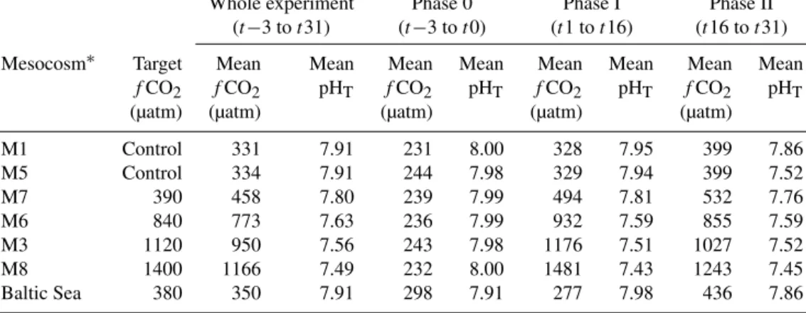
4598 A. L. Webb et al.: Effect of ocean acidification and elevatedfCO2 Table 1.Summary offCO2and pHT(total scale) during phases 0, I, and II of the mesocosm experiment.
Whole experiment Phase 0 Phase I Phase II
(t−3 tot31) (t−3 tot0) (t1 tot16) (t16 tot31)
Mesocosm∗ Target Mean Mean Mean Mean Mean Mean Mean Mean
fCO2 fCO2 pHT fCO2 pHT fCO2 pHT fCO2 pHT
(µatm) (µatm) (µatm) (µatm) (µatm)
M1 Control 331 7.91 231 8.00 328 7.95 399 7.86
M5 Control 334 7.91 244 7.98 329 7.94 399 7.52
M7 390 458 7.80 239 7.99 494 7.81 532 7.76
M6 840 773 7.63 236 7.99 932 7.59 855 7.59
M3 1120 950 7.56 243 7.98 1176 7.51 1027 7.52
M8 1400 1166 7.49 232 8.00 1481 7.43 1243 7.45
Baltic Sea 380 350 7.91 298 7.91 277 7.98 436 7.86
∗Listed in order of increasingfCO2.
selected mesocosm to evaluate the precision of the analysis (< 4 %, no further data shown).
On return to the laboratory, 40 mL of water was in- jected into a purge and cryotrap system (Chuck et al., 2005), filtered through a 25 mm Whatman glass fibre fil- ter (GF/F; GE Healthcare Life Sciences, Little Chalfont, England) and purged with oxygen-free nitrogen (OFN) at 80 mL min−1 for 10 min. Each gas sample passed through a glass wool trap to remove particles and aerosols, before a dual Nafion counterflow drier (180 mL min−1 OFN) re- moved water vapour from the gas stream. The gas sample was trapped in a stainless steel loop held at −150◦C in the headspace of a liquid-nitrogen-filled dewar. The sam- ple was injected by immersion of the sample loop in boil- ing water into an Agilent 6890 gas chromatograph equipped with a 60 m DB-VRX capillary column (0.32 mm ID, 1.8 µm film thickness, Agilent J&W Ltd) according to the pro- gramme outlined by Hopkins et al. (2010). Analysis was performed by an Agilent 5973 quadrupole mass spectrom- eter operated in electron ionisation, single-ion mode. Liq- uid standards of CH3I, diiodomethane (CH2I2), CH2ClI, iodoethane (C2H5I), iodopropane (C3H7I), CHBr3, dibro- moethane (CH2Br2), dibromochloromethane (CHBr2Cl), bromoiodomethane (CH2BrI), and DMS (standards supplied by Sigma Aldrich Ltd, UK) were gravimetrically prepared by dilution in high-performance liquid chromatography (HPLC) grade methanol (Table 2) and used for calibration. The rela- tive standard error was expressed as a percentage of the mean for the sample analysis, calculated for each compound using triplicate analysis each day from a single mesocosm, and was
< 7 % for all compounds. Gas chromatography–mass spec- trometry instrument drift was corrected by the use of a sur- rogate analyte standard in every sample, comprising deuter- ated DMS (D6-DMS), deuterated methyl iodide (CD3I), and
13C dibromoethane (13C2H4Br2) via the method described in Hughes et al. (2006) and Martino et al. (2005). Five-point calibrations were performed weekly for each compound with
Table 2.Calibration ranges and calculated percentage mean relative standard error for the trace gases measured in the mesocosms.
Compound Calibration range % Mean relative (pmol L−1) standard error
DMS 600–29 300∗ 6.33
DMSP 2030–405 900∗
CH3I 0.11–11.2 4.62
CH2I2 5.61–561.0 4.98
C2H5I 0.10–4.91 5.61
CH2ClI 1.98–99.0 3.64
CHBr3 8.61–816.0 4.03
CH2Br2 0.21–20.9 5.30
CHBr2Cl 0.07–7.00 7.20
∗Throughout the rest of this paper, these measurements are given in nmol L−1.
the addition of the surrogate analyte, with a single standard analysed daily to check for instrument drift; linear regression from calibrations typically producedr2> 0.98. All samples measured within the mesocosms were within the concentra- tion ranges of the calibrations (Table 2).
2.2.2 DMSP
Samples for total DMSP (DMSPT)were collected and stored for later analysis by the acidification method of Curran et al. (1998). A 7 mL subsample was collected from the amber glass bottle into an 8 mL glass sample vial (Labhut, Chur- cham, UK), into which 0.35 µL of 50 % H2SO4was added, before storage at ambient temperature. Particulate DMSP (DMSPP) samples were prepared by the gravity filtration of 20 mL of sample through a 47 mm GF/F in a glass fil- ter unit, before careful removal and folding of the GF/F into a 7 mL sample vial filled with 7 mL of Milli-Q water and 0.35 µL of H2SO4 before storage at ambient tempera- ture. Samples were stored for approximately 8 weeks prior
0 400 800 1200 1600 2000
fCO2(μatm)
M1 (346 μatm) M7 (494 μatm) M3 (1075 μatm) M5 (348 μatm) M6 (868 μatm) M8 (1333 μatm) Baltic sea (343 μatm)
CO2addition
7 10 12 15 17
Temperature (°C)
0 1 2 3 4 5 6 7
-5 0 5 10 15 20 25 30 35
Total Chl-ɑ(μg L-1)
t (day)
0 I II
(a)
(b)
(c)
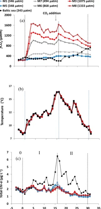
Figure 1.Daily measurements of(a)fCO2,(b)mean temperature, and(c)total chlorophyllain the mesocosms and surrounding Baltic Sea waters. Dashed lines represent the three phases of the experi- ment, based on the Chladata.
to analysis. DMSP samples (total and particulate) were anal- ysed on a PTFE purge and cryotrap system using 2 mL of the sample purged with 1 mL of 10 M NaOH for 5 min at 80 mL min−1. The sample gas stream passed through a glass wool trap and Nafion counterflow (Permapure) drier before being trapped in a PTFE sample loop kept at −150◦C by suspension in the headspace of a liquid nitrogen-filled de- war and controlled by feedback from a thermocouple. Im- mersion in boiling water rapidly re-volatilised the sample for injection into a Shimadzu GC2010 gas chromatograph with a Varian Chrompack CP-Sil-5CB column (30 m, 0.53 mm ID)
and flame photometric detector (FPD). The gas chromatog- raphy (GC) oven was operated isothermally at 60◦C, which resulted in DMS eluting at 2.1 min. Liquid DMSP standards were prepared and purged in the same manner as the sample to provide weekly calibrations of the entire analytical sys- tem. Involvement in the 2013 AQA 12-23 international DMS analysis proficiency test (National Measurement Institute of Australia, 2013) in February 2013 demonstrated excellent agreement between our method of DMSP analysis and the mean from 13 laboratories measuring DMS using different methods, with a measurement error of 5 %.
DMSP was not detected in any of the samples (total or particulate) collected and stored during the experiment, and it was considered likely that this was due to an unre- solved issue regarding acidifying Baltic Sea samples for later DMSP analysis. This method had been used during a previ- ous mesocosm experiment (SOPRAN II, Bergen, Norway), and the results correlated well with those measured immedi- ately on a similar GC-FPD system (Webb et al., 2015). It was considered unlikely that rates of bacterial DMSP turnover through demethylation rather than through cleavage to pro- duce DMS (Curson et al., 2011) were sufficiently high in the Baltic Sea to remove all detectable DMSP yet still pro- duce measurable DMS concentrations. Also, rapid turnover of dissolved DMSP in surface waters being the cause of low DMSPTconcentrations does not explain the lack of intracel- lular particulate-phase DMSP. Although production of DMS is possible from alternate sources, it is highly unlikely that there was a total absence of DMSP-producing phytoplankton within the mesocosms or Baltic Sea surface waters around Tvärminne; DMSP was measured in surface waters of the southern Baltic Sea at 22.2 nmol L−1in 2012, indicating that DMSP-producing species are present within the Baltic Sea (C. Zindler, personal communication, 2014).
A previous study by del Valle et al. (2011) highlighted up to 94 % loss of DMSPT from acidified samples of colonial Phaeocystis globosaculture and field samples dominated by colonialPhaeocystis antarctica. Despite filamentous, colo- nial cyanobacteria in the samples from Tvärminne meso- cosms potentially undergoing the same process, these species did not dominate the community, at only 6.6 % of the total Chla, implying that the acidification method for DMSP fix- ation also failed for unicellular phytoplankton species. The findings of this mesocosm study suggest that the acidifica- tion method is unreliable in the Baltic Sea and should be considered inadequate as the sole method of DMSP fixation in future experiments in the region. The DMSP acidification method is used worldwide as a simple and effective method of DMSP storage; the findings here, alongside those of del Valle et al. (2011), question the applicability of this method in other marine environments and suggest significant testing prior to reliance on this method as a sole means of DMSP storage.
4600 A. L. Webb et al.: Effect of ocean acidification and elevatedfCO2 2.3 Measurement of carbonate chemistry and
community dynamics
Water samples were collected from the 10 and 17 m IWS on a daily basis and analysed for carbonate chemistry, flu- orometric Chla, phytoplankton pigments (17 m IWS only), and cell abundance to analyse the community structure and dynamics during the experiment. The carbonate system was analysed through a suite of measurements (Paul et al., 2015), including potentiometric titration for total alkalinity (TA), in- frared absorption for dissolved inorganic carbon (DIC), and spectrophotometric determination for pH. For Chla analy- sis and pigment determination, 500 mL subsamples were fil- tered through a GF/F and stored frozen (−20◦C for 2 h for Chl a and −80◦C for up to 6 months for pigments), be- fore homogenisation in 90 % acetone with glass beads. After centrifuging (10 min at 800 g at 4◦C) the Chl a concentra- tions were determined using a Turner AU-10 fluorometer by the methods of Welschmeyer (1994), and the phytoplankton pigment concentrations were determined by reverse phase high-performance liquid chromatography (WATERS HPLC with a Varian Microsorb-MV 100-3 C8 column) as described by Barlow et al. (1997). Phytoplankton community compo- sition was determined by the use of the CHEMTAX algo- rithm to convert the concentrations of marker pigments to Chlaequivalents (Mackey et al., 1996; Schulz et al., 2013).
Microbes were enumerated using a Becton Dickinson FAC- SCalibur flow cytometer (FCM) equipped with a 488 nm ar- gon laser (Crawfurd et al., 2016), and counts of phytoplank- ton cells > 20 µm were made on concentrated (50 mL) sample water, fixed with acidic Lugol’s iodine solution with an in- verted microscope. Filamentous cyanobacteria were counted in 50 µm length units.
2.4 Statistical analysis
All statistical analysis was performed using Minitab V16.
In analysis of the measurements between mesocosms, one- way ANOVA was used with Tukey’s post hoc analysis test to determine the effect of differentfCO2on concentrations measured in the mesocosms and the Baltic Sea (H0assumes no significant difference in the mean concentrations of trace gases measured through the duration of the experiment).
Spearman’s rank correlation coefficients were calculated to compare the relationships between trace gas concentrations, fCO2, and a number of biological parameters, and the re- sultingρvalues for each correlation are given in Supplement Table S1 for the mesocosms and Table S2 for the Baltic Sea data.
0
2 4 6 8 10 12
-5 0 5 10 15 20 25 30 35
DMS (nmol L-1)
t (day)
M1 (346 μatm) M7 (494 μatm) M3 (1075 μatm) M5 (348 μatm) M6 (868 μatm) M8 (1333 μatm) Baltic (343 μatm)
2 3 4 5 6 7
0 500 1000 1500 2000
DMS (nmol L-1)
fCO2(μatm) (a)
(b)
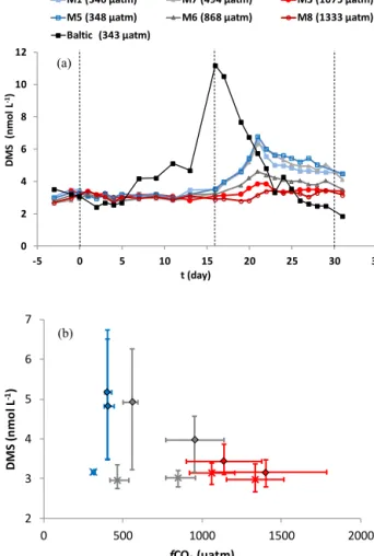
Figure 2. (a)Mean DMS concentrations measured daily in the mesocosms and Baltic Sea from an integrated water sample of the surface 10 m. Dashed lines show the phases of the experiment as given in Fig. 1;fCO2shown in the legend is meanfCO2across the duration of the experiment.(b)Mean DMS concentrations from each mesocosm during Phase I (crosses) and Phase II (diamonds), for ambient (blue), medium (grey), and highfCO2(red), with error bars showing the range of both the DMS andfCO2.
3 Results and discussion
3.1 Biogeochemical changes within the mesocosms The mesocosm experiment was split into three phases based on the temporal variation in Chla (Fig. 2; Paul et al., 2015) evaluated after the experiment was completed:
– Phase 0 (dayst−5 tot0) – pre-CO2addition;
– Phase I (dayst1 tot16) – “productive phase”;
– Phase II (dayst17 to t30) – temperature-induced au- totrophic decline.
3.1.1 Physical parameters
fCO2 decreased over Phase I in the three highest-fCO2 mesocosms, mainly through air–sea gas exchange and car- bon fixation by phytoplankton (Fig. 1a). All mesocosms still showed distinct differences in fCO2 levels throughout the experiment (Table 1), and there was no overlap of mesocosm fCO2values on any given day, save for the two controls (M1 and M5). The control mesocosm fCO2 increased through Phase I of the experiment, likely as a result of undersatura- tion of the water column encouraging dissolution of atmo- spheric CO2(Paul et al., 2015). Salinity in the mesocosms remained constant throughout the experiment at 5.70±0.004 and showed no variation with depth (data not shown but available in Paul et al., 2015). It remained similar to salin- ity in the Baltic Sea surrounding the mesocosms, which was 5.74±0.14. Water temperature varied from a low of 8.6±0.4◦C during Phase 0 to a high of 15.9±2.2◦C mea- sured on dayt16, before decreasing once again (Fig. 1b).
Summertime upwelling events are common and well de- scribed (Gidhagen, 1987; Lehmann and Myrberg, 2008) and induce a significant temperature decrease in surface waters;
such an event appears to have commenced aroundt16, as in- dicated by significantly decreasing temperatures inside and out of the mesocosms (Fig. 1b) and increased salinity in the Baltic Sea from 5.5 to 6.1 over the following 15 days to the end of the experiment. Due to the enclosed nature of the mesocosms, the upwelling affected only the temperature and not pH, fCO2, or the microbial community. However, the temperature decrease aftert16 was likely to have had a significant effect on phytoplankton growth (and biogenic gas production), explaining the lower Chlain Phase II.
3.1.2 Community dynamics
Mixing of the mesocosms and redistribution of the nutrients throughout the water column after closure (prior tot−3) did not trigger a notable increase in total Chl a in Phase 0 as was identified in previous mesocosm experiments. During Phase I, light availability, combined with increasing water temperatures, favoured the growth of phytoplankton in all mesocosms (Paul et al., 2015) and was unlikely to be a direct result of the CO2enrichment, as no difference was identified between enriched mesocosms and controls. Mean Chladur- ing Phase I was 1.98 (±0.29) µg L−1 from all mesocosms, decreasing to 1.44 (±0.46) µg L−1in Phase II; this decrease was attributed to a temperature-induced decreased in phyto- plankton growth rates and higher grazing rates as a result of higher zooplankton reproduction rates during Phase I (Lis- chka et al., 2015; Paul et al., 2015). Mesocosm Chl a de- creased until the end of the experiment ont31.
The largest contributors to Chlain the mesocosms during the summer of 2012 were the chlorophytes and cryptophytes, with up to 40 and 21 % contributions to the Chlarespectively (Table 3; Paul et al., 2015). Significant long-term differences
in abundance between mesocosms developed as a result of elevatedfCO2in only two groups: picoeukaryotes I showed higher abundance at highfCO2 (F =8.2,p<0.01; Craw- furd et al., 2016, and Supplement Fig. S2), as seen in pre- vious mesocosm experiments (Brussaard et al., 2013; New- bold et al., 2012), and picoeukaryotes III showed the opposite trend (F=19.6,p<0.01; Crawfurd et al., 2016). Temporal variation in phytoplankton abundance was similar between all mesocosms (Figs. S1 and S2).
Diazotrophic, filamentous cyanobacterial blooms in the Baltic Sea are an annual event in summer (Finni et al., 2001), and single-celled cyanobacteria have been found to comprise as much as 80 % of the cyanobacterial biomass and 50 % of the total primary production during the summer in the Baltic Sea (Stal et al., 2003). However, CHEMTAX analysis identi- fied cyanobacteria as contributing less than 10 % of the total Chla in the mesocosms (Crawfurd et al., 2016; Paul et al., 2015). These observations were backed up by satellite obser- vations showing reduced cyanobacterial abundance through- out the Baltic Sea in 2012 compared to previous and later years (Oberg, 2013). It was proposed that light availability and surface water temperatures during the summer of 2012 were suboptimal for triggering a filamentous cyanobacteria bloom (Wasmund, 1997).
3.2 DMS and DMSP 3.2.1 Mesocosm DMS
A significant 34 % reduction in DMS concentrations was detected in the high-fCO2 treatments during Phase II compared to the ambient-fCO2 mesocosms (F=31.7, p<0.01). Mean DMS concentrations of 5.0 (±0.8; range 3.5–6.8) nmol L−1in the ambient treatments were compared to 3.3 (±0.3; range 2.9–3.9) nmol L−1 in the 1333 and 1075 µatm mesocosms (Fig. 2a). The primary differences identified were apparent from the start of Phase II ont17, after which maximum concentrations were observed in the ambient mesocosms ont21. The relationship between DMS and increasingfCO2 during Phase II was found to be lin- ear (Fig. 2b), a finding also identified in previous mesocosm experiments (Archer et al., 2013; Webb et al., 2015). Further- more, increases in DMS concentrations under highfCO2
were delayed by 3 days relative to the ambient- and medium- fCO2treatments, a situation which has been observed in a previous mesocosm experiment. This was attributed to small- scale shifts in community composition and succession which could not be identified with only a once-daily measurement regime (Vogt et al., 2008). DMS measured in all mesocosms fell within the range 2.7 to 6.8 nmol L−1across the course of the experiment. During Phase I, no difference was identified in DMS concentrations betweenfCO2treatments, with the mean of all mesocosms being 3.1 (±0.2) nmol L−1. Concen- trations in all mesocosms gradually declined fromt21 until the end of DMS measurements ont31. DMS concentrations
4602 A. L. Webb et al.: Effect of ocean acidification and elevatedfCO2 Table 3.Abundance and contributions of different phytoplankton groups to the total phytoplankton community assemblage, showing the range of measurements from total Chla(Paul et al., 2015), CHEMTAX analysis of derived Chla(Paul et al., 2015), and phytoplankton abundance (Crawfurd et al., 2016). Data are split into the range of all the mesocosm measurements and those from the Baltic Sea.
Mesocosm Baltic Sea
Range Range % contribution Range Range % contribution
Integrated 10 m Integrated 17 m to Chla Integrated 10 m Integrated 17 m to Chla
Chla 0.9–2.9 0.9–2.6 100 1.3–6.5 1.12–5.5 100
Phytoplankton taxonomy (equivalent chlorophyll µg L−1)
Cyanobacteria 0.01–0.4 8 0.0–0.1 1
Prasinophytes 0.04–0.3 7 0.01–0.3 4
Euglenophytes 0.0–1.6 15 0.0–2.6 21
Dinoflagellates 0.0–0.3 3 0.04–0.6 9
Diatoms 0.1–0.3 7 0.04–0.9 9
Chlorophytes 0.3–2.0 40 0.28–3.1 41
Cryptophytes 0.1–1.4 21 0.1–1.0 15
Small phytoplankton (< 10 µm) abundance (cells mL−1)
Cyanobacteria 55 000–380 000 65 000–470 000 30 000–180 000 30 000–250 000
Picoeukaryotes I 15 000–10 0000 17 000–111 000 5000–70 000 6100–78 000
Picoeukaryotes II 700–4000 600–4000 400–3000 460–3700
Picoeukaryotes III 1000–9000 1100–8500 1000–6000 950–7500
Nanoeukaryotes I 400–1400 270–1500 200–4000 210–4100
Nanoeukaryotes II 0–400 4–400 100–1100 60–1300
measured in the mesocosms and Baltic Sea were compara- ble to those measured in temperate coastal conditions in the North Sea (Turner et al., 1988), the Mauritanian upwelling (Franklin et al., 2009; Zindler et al., 2012), and the South Pacific (Lee et al., 2010).
The majority of DMS production is presumed to be from DMSP. However, an alternative production route for DMS is available through the methylation of methanethiol (Drotar et al., 1987; Kiene and Hines, 1995; Stets et al., 2004), predom- inantly identified in anaerobic environments such as fresh- water lake sediments (Lomans et al., 1997), salt marsh sedi- ments (Kiene and Visscher, 1987), and microbial mats (Viss- cher et al., 2003; Zinder et al., 1977). Recent studies have also identified this pathway of DMS production fromPseu- domonas deceptionensisin an aerobic environment (Carrión et al., 2015), where P. deceptionensis was unable to syn- thesise or catabolise DMSP but was able to enzymatically mediate DMS production from methanethiol (MeSH). The same enzyme has also been identified in a wide range of other bacterial taxa, including the cyanobacterialPseudan- abaena, which was identified in the Baltic Sea during this and previous investigations (A. Stuhr, personal communica- tion, 2015; Kangro et al., 2007; Nausch et al., 2009). Cor- relations between DMS and the cyanobacterial equivalent Chla (ρ=0.42, p<0.01; Fig. S1g) and DMS and single- celled cyanobacteria (ρ=0.58,p<0.01; Fig. S2a) suggest that the methylation pathway may be a potential source of DMS within the Baltic Sea community. In addition to the
methylation pathway, DMS production has been identified from S-methylmethionine (Bentley and Chasteen, 2004), as well as from the reduction of dimethylsulfoxide (DMSO), in both surface and deep waters by bacterial metabolism (Hat- ton et al., 2004). As these compounds were not measured in the mesocosms, it is impossible to determine whether they were significant sources of DMS.
3.2.2 DMS and community interactions
Throughout Phase I, DMS showed no correlation with any measured variables of biological activity or cell abundance and was unaffected by elevatedfCO2, indicating that mea- sured DMS concentrations were not directly related to the perturbation of the system and associated cellular stress (Sunda et al., 2002). Of the studied phytoplankton group- ings, neither the cryptophytes nor chlorophytes as the largest contributors of Chlawere identified as significant producers of DMSP. During Phase II, DMS was negatively correlated with Chla in the ambient- and medium-fCO2mesocosms (ρ= −0.60,p<0.01). During Phase II, a significant corre- lation was seen between DMS and single-celled cyanobac- teria identified predominantly asSynechococcus (ρ=0.53, p<0.01; Crawfurd et al., 2016, and Table S1) and pi- coeukaryotes III (ρ=0.75,p<0.01). The peak in DMS con- centrations ont21 is unlikely to be a delayed response to the increased Chla ont16 due to the time lag of 7 days. These higher DMS concentrations were likely connected to a peak
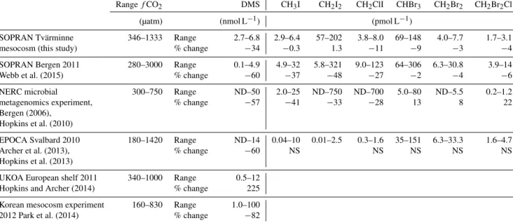
Table 4.Concentration ranges of trace gases measured in the mesocosms compared to other open-water ocean acidification experiments, showing the range of concentrations for each gas and the percentage change between the control and the highest-fCO2treatment. SOPRAN:
Surface Ocean Processes in the Anthropocene; NERC: Natural Environment Research Council; EPOCA: European Project on OCean Acid- ification; UKOA: UK Ocean Acidification Research Programme.
RangefCO2 DMS CH3I CH2I2 CH2ClI CHBr3 CH2Br2 CH2Br2Cl
(µatm) (nmol L−1) (pmol L−1)
SOPRAN Tvärminne 346–1333 Range 2.7–6.8 2.9–6.4 57–202 3.8–8.0 69–148 4.0–7.7 1.7–3.1
mesocosm (this study) % change −34 −0.3 1.3 −11 −9 −3 −4
SOPRAN Bergen 2011 280–3000 Range 0.1–4.9 4.9–32 5.8–321 9.0–123 64–306 6.3–30.8 3.9–14
Webb et al. (2015) % change −60 −37 −48 −27 −2 −4 −6
NERC microbial 300–750 Range ND–50 2.0–25 ND–750 ND–700 5.0–80 ND–5.5 0.2–1.2
metagenomics experiment, % change −57 −41 −33 −28 13 8 22
Bergen (2006), Hopkins et al. (2010)
EPOCA Svalbard 2010 180–1420 Range ND–14 0.04–10 0.01–2.5 0.3–1.6 35–151 6.3–33.3 1.6–4.7
Archer et al. (2013), % change −60 NS NS NS NS NS
Hopkins et al. (2013)
UKOA European shelf 2011 340–1000 Range 0.5–12
Hopkins and Archer (2014) % change 225
Korean mesocosm experiment 160–830 Range 1.0–100
2012 Park et al. (2014) % change −82
ND – not detected.
NC – no change.
in dissolved organic carbon (DOC) on t15, as well as in- creasing bacterial abundance during Phase II (Hornick et al., 2016). It is also likely that DMS concentrations increased as a response to the mesocosm wall cleaning which took place ont16. The variation in inorganic nutrient concentrations be- tween mesocosms at the start of the experiment did not have an effect on DMS concentrations during Phase I, and by the start of Phase II the variation between mesocosms had de- creased.
In previous mesocosm experiments (Archer et al., 2013;
Hopkins et al., 2010; Webb et al., 2015), DMS has shown poor correlations with many of the indicators of primary pro- duction and phytoplankton abundance, as well as showing the same trend of decreased concentrations in high-fCO2 mesocosms compared to ambient ones. DMS production is often uncoupled from measurements of primary production in open waters (Lana et al., 2012) and also often from the production of its precursor DMSP (Archer et al., 2009). DMS and DMSP are important sources of sulfur and carbon in the microbial food web for both bacteria and algae (Simó et al., 2002, 2009), and since microbial turnover of DMSP and DMS play a significant role in net DMS production, it is unsurprising that DMS concentrations have shown poor cor- relation with DMSP-producing phytoplankton groups in past experiments and open waters.
DMS concentrations have been reported to be lower under conditions of elevatedfCO2compared to ambient controls, in both mesocosm experiments (Table 4) and phytoplankton monocultures (Arnold et al., 2013; Avgoustidi et al., 2012).
However, the varying response of the community within each experiment limits our ability to generalise the response of al- gal production of DMS and DMSP in all situations due to the characteristic community dynamics of each experiment in specific geographical areas and temporal periods. Previ- ous experiments in the temperate Raunefjorden of Bergen, Norway, showed lower abundance of DMSP-producing algal species, and subsequently of DMSP-dependent DMS con- centrations (Avgoustidi et al., 2012; Hopkins et al., 2010;
Vogt et al., 2008; Webb et al., 2015). In contrast mesocosm experiments in the Arctic and Korea have shown increased abundance of DMSP producers (Archer et al., 2013; Kim et al., 2010) but lower DMS concentrations, while incubation experiments by Hopkins and Archer (2014) showed lower DMSP production but higher DMS concentrations at high fCO2. However, in all previous experiments with DMSP as the primary precursor of DMS, elevated fCO2 had a less marked effect on measured DMSP concentrations than on measured DMS concentrations. Hopkins et al. (2010) sug- gested that “the perturbation of the system has a greater ef- fect on the processes that control the conversion of DMSP to DMS rather than the initial production of DMSP itself”.
Previous mesocosm experiments have suggested signifi- cant links between increased bacterial production through greater availability of organic substrates at highfCO2(En- gel et al., 2013; Piontek et al., 2013). Further, Endres et al. (2014) identified significant enhanced enzymatic hydrol- ysis of organic matter with increasing fCO2, with higher bacterial abundance. Higher bacterial abundance will likely
4604 A. L. Webb et al.: Effect of ocean acidification and elevatedfCO2
0 1 2 3 4 5 6 7 8 9 10
-5 0 5 10 15 20 25 30 35
CH3I (pmol L-1)
t (day)
M1 (346 μatm) M7 (494 μatm) M3 (1075 μatm) M5 (348 μatm) M6 (868 μatm) M8 (1333 μatm) Baltic (343 μatm)
0.0 0.2 0.4 0.6 0.8 1.0 1.2
-5 0 5 10 15 20 25 30 35
C2H5I (pmol L-1)
t (Day)
0 50 100 150 200 250 300 350 400
-5 0 5 10 15 20 25 30 35
CH2I2(pmol L-1)
t (day)
0 4 8 12 16 20
-5 0 5 10 15 20 25 30 35
CH2ClI (pmol L-1)
t (day)
(a) (b)
(c) (d)
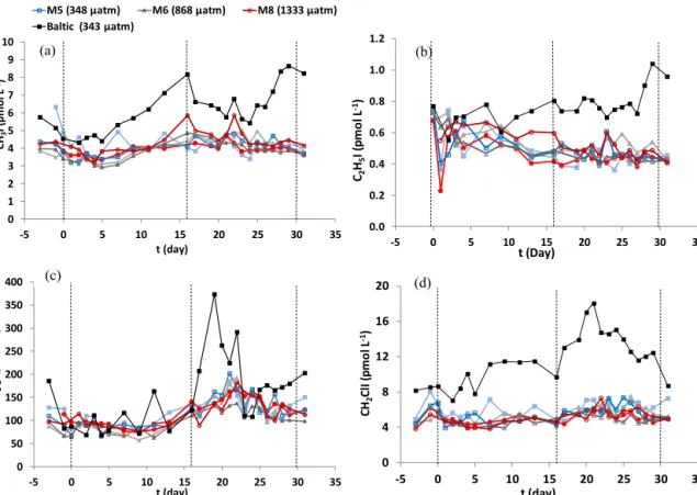
Figure 3.Mean concentrations (pmol L−1)of(a)CH3I,(b)C2H5I,(c)CH2I2, and(d)CH2ClI taken from a water sample integrated from the surface 10 m. Dashed lines indicate the phases of the experiment, as given in Fig. 2.fCO2shown in the legend is meanfCO2across the duration of the experiment.
result in greater bacterial demand for sulfur and therefore greater consumption of DMS and conversion to DMSO. This was suggested as a significant sink for DMS in a previous experiment (Webb et al., 2015), but during the present ex- periment, both bacterial abundance and bacterial production were lower at high fCO2(Hornick et al., 2016). However, as it has been proposed that only specialist bacterial groups are DMS consumers (Vila-Costa et al., 2006b) and there is no determination of the DMS consumption characteristics of the bacterial community in the Baltic Sea, it is not known if this loss pathway is stimulated at highfCO2. As microbial DMS yields can vary between 5 and 40 % depending on the sul- fur and carbon demand (Kiene and Linn, 2000), a change in the bacterial sulfur requirements could change DMS turnover despite lower abundance.
3.3 Iodocarbons in the mesocosms and relationships with community composition
ElevatedfCO2did not affect the concentration of iodocar- bons in the mesocosms significantly at any time during the experiment, which is in agreement with the findings of Hop- kins et al. (2013) in the Arctic but in contrast to Hopkins et al. (2010) and Webb (2015), where iodocarbons were
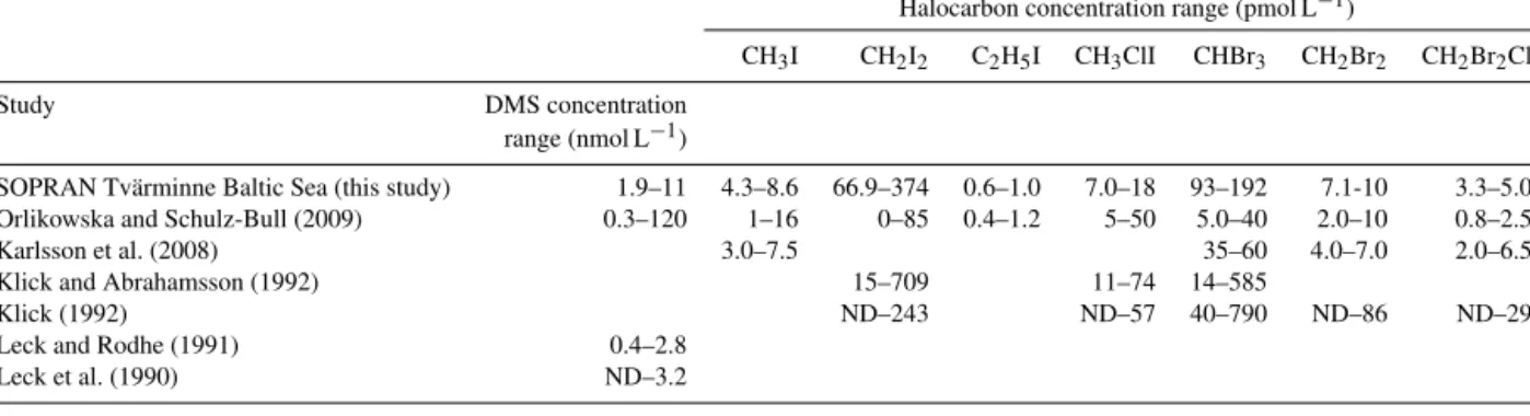
measured to be significantly lower under elevated fCO2 (Table 4). Concentrations of all iodocarbons measured in the mesocosms and the Baltic Sea fall within the range of those measured previously in the region (Table 5). Meso- cosm concentrations of CH3I (Fig. 3a) and C2H5I (Fig. 3b) showed concentration ranges of 2.91 to 6.25 and 0.23 to 0.76 pmol L−1 respectively. CH3I showed a slight increase in all mesocosms during Phase I, peaking on t16, which corresponded to higher Chla concentrations and correlated throughout the entire experiment with picoeukaryote groups II (ρ=0.59,p<0.01) and III (ρ=0.23,p<0.01; Crawfurd et al., 2016) and nanoeukaryotes I (ρ=0.37,p<0.01). Sig- nificant differences identified between mesocosms for CH3I were unrelated to elevated fCO2 (F=3.1, p<0.05), but concentrations were on average 15 % higher in Phase II than Phase I. C2H5I decreased slightly during Phases I and II, al- though concentrations of this halocarbon were close to its detection limit (0.2 pmol L−1), remaining below 1 pmol L−1 at all times. As this compound showed no significant ef- fect of elevatedfCO2and was identified by Orlikowska and Schulz-Bull (2009) as having extremely low concentrations in the Baltic Sea (Table 5), it will not be discussed further.
Table 5.Concentration ranges of trace gases measured in the Baltic Sea compared to concentrations measured in the literature.
Halocarbon concentration range (pmol L−1)
CH3I CH2I2 C2H5I CH3ClI CHBr3 CH2Br2 CH2Br2Cl
Study DMS concentration
range (nmol L−1)
SOPRAN Tvärminne Baltic Sea (this study) 1.9–11 4.3–8.6 66.9–374 0.6–1.0 7.0–18 93–192 7.1-10 3.3–5.0 Orlikowska and Schulz-Bull (2009) 0.3–120 1–16 0–85 0.4–1.2 5–50 5.0–40 2.0–10 0.8–2.5
Karlsson et al. (2008) 3.0–7.5 35–60 4.0–7.0 2.0–6.5
Klick and Abrahamsson (1992) 15–709 11–74 14–585
Klick (1992) ND–243 ND–57 40–790 ND–86 ND–29
Leck and Rodhe (1991) 0.4–2.8
Leck et al. (1990) ND–3.2
ND – not detected.
No correlation was found between CH3I and Chlaat any phase, and the only correlation of any phytoplankton group- ing was with nanoeukaryotes II (ρ=0.88,p<0.01; Craw- furd et al., 2016). These CH3I concentrations compare well to the 7.5 pmol L−1measured by Karlsson et al. (2008) dur- ing a cyanobacterial bloom in the Baltic Sea (Table 5) and the summer maximum of 16 pmol L−1identified by Orlikowska and Schulz-Bull (2009).
Karlsson et al. (2008) showed Baltic Sea halocarbon pro- duction occurring predominately during daylight hours, with concentrations at night decreasing by 70 % compared to late afternoon. Light-dependent production of CH3I has been shown to take place through abiotic processes, including radical recombination of CH3 and I (Moore and Zafiriou, 1994). However, since samples were integrated over the sur- face 10 m of the water column, it was impossible to deter- mine whether photochemistry was affecting iodocarbon con- centrations near the surface where some UV light was able to pass between the top of the mesocosm film material and the cover. For the same reason, photodegradation of halo- carbons (Zika et al., 1984) within the mesocosms was also likely to have been significantly restricted. Thus, as photo- chemical production was expected to be minimal, biogenic production was likely to have been the dominant source of these compounds. Karlsson et al. (2008) identifiedPseudan- abaenaas a key producer of CH3I in the Baltic Sea. However, the abundance ofPseudanabaenawas highest during Phase I of the experiment (A. Stuhr, personal communication, 2015) when CH3I concentrations were lower, and as discussed pre- viously, the abundance of these species constituted only a very small proportion of the community. Previous investiga- tions in the laboratory have identified diatoms as significant producers of CH3I (Hughes et al., 2013; Manley and De La Cuesta, 1997), and the low, steady-state abundance of the di- atom populations in the mesocosms could have produced the same relatively steady-state trends in the iodocarbon concen- trations.
Measured in the range 57.2–202.2 pmol L−1in the meso- cosms, CH2I2 (Fig. 3c) showed the clearest increase in
concentration during Phase II, when it peaked on t21 in all mesocosms, with a maximum of 202.2 pmol L−1 in M5 (348 µatm). During Phase II, concentrations of CH2I2were 57 % higher than Phase I and were therefore negatively cor- related with Chl a. The peak on t21 corresponds to the peak identified in DMS ont21, and concentrations through all three phases correlate with picoeukaryotes II (ρ=0.62, p<0.01) and III (ρ=0.47,p<0.01) and nanoeukaryotes I (ρ=0.88,p<0.01; Crawfurd et al., 2015). CH2ClI (Fig. 3d) showed no peaks during either Phase I or Phase II, remaining within the range of 3.81 to 8.03 pmol L−1and again corre- lated with picoeukaryotes groups II (ρ=0.34,p<0.01) and III (ρ=0.38,p<0.01). These results may suggest that these groups possessed halo-peroxidase enzymes able to oxidise I−, most likely as an antioxidant mechanism within the cell to remove H2O2(Butler and Carter-Franklin, 2004; Pedersen et al., 1996; Theiler et al., 1978). However, given the lack of response of these compounds to elevatedfCO2(F =1.7, p<0.01), it is unlikely that production was increased in re- lation to elevatedfCO2. Production of all iodocarbons in- creased during Phase II when total Chl a decreased, par- ticularly after the walls of the mesocosms were cleaned for the first time, releasing significant volumes of organic ag- gregates into the water column. Aggregates have been sug- gested as a source of CH3I and C2H5I (Hughes et al., 2008), likely through the alkylation of inorganic iodide (Urhahn and Ballschmiter, 1998) or through the breakdown of organic matter by microbial activity to supply the precursors required for iodocarbon production (Smith et al., 1992). Hughes et al. (2008) did not identify this route as a pathway for CH2I2
or CH2ClI production, but Carpenter et al. (2005) suggested a production pathway for these compounds through the reac- tion of HOI with aggregated organic materials.
3.4 Bromocarbons in the mesocosms and the relationships with community composition
No effect of elevated fCO2 was identified for any of the three bromocarbons, which compared well with the findings from previous mesocosms where bromocarbons were studied
4606 A. L. Webb et al.: Effect of ocean acidification and elevatedfCO2 (Hopkins et al., 2010, 2013; Webb, 2015; Table 4). Measured
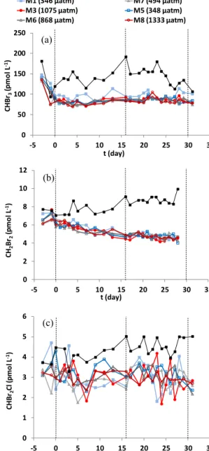
concentrations were comparable to those of Orlikowska and Schulz-Bull (2009) and Karlsson et al. (2008) measured in the southern part of the Baltic Sea (Table 3). The concen- trations of CHBr3, CH2Br2, and CHBr2Cl showed no ma- jor peaks of production in the mesocosms. CHBr3(Fig. 4a) decreased rapidly in all mesocosms over Phase 0 from a maximum measured concentration of 147.5 pmol L−1in M1 (mean of 138.3 pmol L−1 in all mesocosms) to a mean of 85.7 (±8.2 SD) pmol L−1in all mesocosms for the periodt0 tot31 (Phases I and II). The steady-state CHBr3concentra- tions indicated a production source; however, there was no clear correlation with any measured algal groups. CH2Br2
concentrations (Fig. 4b) decreased steadily in all mesocosms fromt−3 through tot31, over the range 4.0 to 7.7 pmol L−1, and CHBr2Cl followed a similar trend in the range 1.7 to 4.7 pmol L−1 (Fig. 4c). Of the three bromocarbons, only CH2Br2 showed correlation with total Chl a (ρ=0.52, p<0.01) and with cryptophyte (ρ=0.86,p<0.01) and di- noflagellate (ρ=0.65,p<0.01)-derived Chla. Concentra- tions of CH2BrI were below detection limit for the entire ex- periment.
CH2Br2showed positive correlation with Chla(ρ=0.52, p<0.01), nanoeukaryotes II (ρ=0.34,p<0.01), and cryp- tophytes (ρ=0.86, p<0.01; see Supplement), whereas CHBr3 and CHBr2Cl showed very weak or no correlation with any indicators of algal biomass. Schall et al. (1997) have proposed that CHBr2Cl is produced in seawater by the nucleophilic substitution of bromide by chloride in CHBr3, which given the steady-state concentrations of CHBr3would explain the similar distribution of CHBr2Cl concentrations.
Production of all three bromocarbons was identified from large-size cyanobacteria such asAphanizomenon flos-aquae by Karlsson et al. (2008), and in addition, significant correla- tions were found in the Arabian Sea between the abundance of the cyanobacteriumTrichodesmiumand several bromocar- bons (Roy et al., 2011), and the low abundance of such bac- teria in the mesocosms would explain the low variation in bromocarbon concentrations through the experiment.
Halocarbon loss processes such as nucleophilic substitu- tion (Moore, 2006), hydrolysis (Elliott and Rowland, 1995), sea–air exchange, and microbial degradation are suggested as of greater importance than the production of these com- pounds by specific algal groups, particularly given the rela- tively low growth rates and low net increase in total Chla.
Hughes et al. (2013) identified bacterial inhibition of CHBr3
production in laboratory cultures of Thalassiosira diatoms but that it was not subject to bacterial breakdown, which could explain the relative steady state of CHBr3 concen- trations in the mesocosms. In contrast, significant bacterial degradation of CH2Br2 in the same experiments could ex- plain the steady decrease in CH2Br2concentrations seen in the mesocosms. Bacterial oxidation was also identified by Goodwin et al. (1998) as a significant sink for CH2Br2. As discussed for the iodocarbons, photolysis was unlikely due
0 50 100 150 200 250
-5 0 5 10 15 20 25 30 35
CHBr3(pmol L-1)
t (day)
M1 (346 μatm) M7 (494 μatm) M3 (1075 μatm) M5 (348 μatm) M6 (868 μatm) M8 (1333 μatm)
0 2 4 6 8 10 12
-5 0 5 10 15 20 25 30 35
CH2Br2(pmol L-1)
t (day)
0 1 2 3 4 5 6
-5 0 5 10 15 20 25 30 35
CHBr2Cl (pmol L-1)
t (day) (a)
(c) (b)
Figure 4. Mean concentrations (pmol L−1) of (a) CHBr3, (b)CH2Br2, and(c)CHBr2Cl taken from a water sample integrated from the surface 10 m. Dashed lines indicate the phases of the ex- periment as defined in Fig. 2;fCO2shown in the legend is mean fCO2across the duration of the experiment.
to the UV absorption of the mesocosm film and limited UV exposure of the surface waters within the mesocosm due to the mesocosm cover. The ratio of CH2Br2to CHBr3was also unaffected by increasedfCO2, staying within the range 0.04 to 0.08. This range in ratios is consistent with that calculated by Hughes et al. (2009) in the surface waters of an Antarctic depth profile and attributed to higher sea–air flux of CHBr3 than CH2Br2 due to a greater concentrations gradient, de- spite the similar transfer velocities of the two compounds (Quack et al., 2007). Using cluster analysis in a time series in the Baltic Sea, Orlikowska and Schulz-Bull (2009) identified