CO 2 Profiling in the Lower Troposphere using a High Spectral Resolution Infrared
Radiometer
Inaugural-Dissertation zur
Erlangung des Doktorgrades
der Mathematisch-Naturwissenschaftlichen Fakult¨ at der Universit¨ at zu K¨ oln
vorgelegt von
Kobra Khosravian Ghadikolaei aus Ghaemshahr
K¨ oln
2017
Berichterstatter: PD. Dr. U. L¨ohnert Prof. Dr. A. Wahner Dr. D. D. Turner Tag der m¨undlichen Pr¨ufung:
16.10.2017
Abstract
The rapid increase of CO2 concentration in the atmosphere due to the anthropogenic activi- ties since the beginning of the industrial revolution in 1750 makes CO2 the most important anthropogenic atmospheric trace gas. Improvements in space-based and ground-based in- strumentation during the last decades provide a high potential to observe atmospheric CO2 spatial and temporal variability in unprecedented details. The interaction of atmospheric CO2 with the terrestrial ecosystem such as plant photosynthesis and soil respiration can produce a considerable diurnal change in the CO2 concentration near the surface. The mea- surement of this diurnal evolution would provide a valuable tool to study the land-vegetation interaction with the atmospheric CO2. Such a tool would also be useful to help evaluate the output of numerical models which predict the CO2 flux near the surface. However, despite all improvements in the measurement capability, capturing this diurnal change in the boundary layer still remains a challenge.
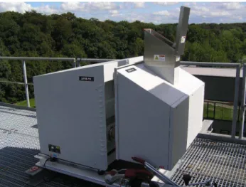
One possibility to improve the observation of the diurnal CO2 cycle is to use the Fourier Transform InfraRed (FTIR) spectrometer. One example of ground-based FTIR spectrom- eter is Atmospheric Emitted Radiance Interferometer (AERI). The AERI was installed in 2011, at J¨ulich ObservatorY for Cloud Evolution (JOYCE), in Germany. It measures the downwelling atmospheric radiation in the mid-infrared region from 520 cm−1 (19µm) to 3020 cm−1 (3.3µm). High temporal (less than 30 s) and spectral (better than 1 cm−1) resolution as well as continuous measurements of the AERI give the opportunity to retrieve the atmo- spheric thermodynamic profiles and cloud properties. In addition, the AERI also observes the emission from several trace gas absorption bands, such as the 15µm CO2 band. These bands can be used to provide useful information about the atmospheric concentration of these trace gases. In the present work, the ability to retrieve profiles of CO2 over the diurnal cycle from AERI-observed radiances is investigated. For this purpose, an algorithm, called AERIoe is utilized and modified to retrieve the CO2 profile in the boundary layer.
Prior to applying the AERIoe to real AERI measurements, simulated radiances are used to evaluate the potential of retrieving atmospheric CO2 concentration from AERI radiance ob- servations. A line-by-line radiative transfer model (LBLRTM) using numerical model profiles as input are utilized to compute downwelling radiances, which are convolved with the instru- ment function and random noise added in order to simulate an AERI observation. In the first step, a constant atmospheric mixing ratio is considered for the atmospheric CO2 profile.
AERIoe results show about 2 ppm overestimation in retrieving the constant CO2 mixing ratio. In order to improve the results, reduced noise, which can be interpreted as using tem- porally averaged AERI radiances, is added to the simulated radiances. These results show considerable improvement compared to the previous results where by ∼70% of the retrieved values are within the expected uncertainty. However, a constant atmospheric profile can not provide any information related to the diurnal change of CO2 concentration near the surface,
i
ii
meaning that a profile which can represent the diurnal CO2 variation needs to be retrieved.
Due to the low numbers of degrees of freedom for signal in retrieving the CO2 concentration, the CO2 profile is parametrized using an exponential function. This exponential function gives the opportunity to calculate the CO2 profile by retrieving 2 shape parameters, rather than retrieving whole profile.
In order to evaluate the modified AERIoe, simulated radiances with the reduced noise for one month are provided to the algorithm. The AERIoe is then run while temperature and humidity profiles are considered as known profiles. The CO2 concentrations in different levels are captured quite accurately by the algorithm where the root mean square values between true and retrieved CO2 concentrations are 6.8, 5.4, 4.0 and 1.9 ppm at the surface, 90 m, 200 m and 1 km respectively. The retrieved profiles improved the root mean square between true and prior profiles by ∼ 50%. The algorithm is then used to retrieve the temperature, humidity and CO2 profiles simultaneously. These results show a significant reduction in the CO2 degrees of freedom which causes poor retrieval results. Consequently, a second method is used wherein a principal component noise filter is applied to reduce the random error in the AERI observations. High temporal resolution simulated radiances are used to test the new method. The results of the AERIoe run with the noise-filtered radiances demonstrate considerable improvement in retrieving the CO2 concentration near the surface.
The AERIoe is then applied to real AERI observations from two clear sky days at J¨ulich to retrieve profiles of CO2. The tower in-situ measurements at J¨ulich are utilized to compare with the retrieved CO2 concentration near the surface. It is shown that the AERI radiances have the potential to capture the diurnal variation of the CO2concentration near the surface.
The retrieved values for the surface CO2 concentration show between 5 to 10 ppm difference with the tower measurements during these two days, while the uncertainties in the retrieved values are between 4 to 7 ppm. The AERI radiances are also used to estimate the height where the CO2 concentration deviates from its background value. The diurnal change of the derived heights for one of these two days are in good agreement with the expected diurnal change of the boundary layer for a sunny and clear sky day.
Zusammenfassung
Der schnelle Anstieg der CO2 Konzentration in der Atmosph¨are, der seit dem Beginn der industriellen Revolution ab 1750 durch anthropogene Aktivit¨aten hervorgerufen wird, macht CO2 zum wichtigsten anthropogenen Spurengas der Atmosph¨are. Fortschritte der satelliten- und bodengest¨utzten Messtechnik in den letzten Jahrzehnten bieten ein hohes Potential, die r¨aumliche und zeitliche Ver¨anderung von atmosph¨arischem CO2 in noch nie da gewe- senem Detail zu erfassen. Das Zusammenspiel von atmosph¨arischem CO2 und dem irdischen Okosystem, zum Beispiel durch Pflanzenphotosynthese und Bodenatmung, kann einen er-¨ heblichen Tagesgang in der oberfl¨achennahen CO2 Konzentration verursachen. Messungen dieses Tagesgangs w¨aren ein wertvolles Hilfsmittel zur Untersuchung des Zusammenspiels von Land und Vegetation mit dem atmosph¨arischen CO2. Ein solches Hilfsmittel k¨onnte außerdem eine Beurteilung von numerischen Modellen, die den oberfl¨achennahen CO2 Fluss vorhersagen, erm¨oglichen. Trotz Verbesserung der Messungm¨oglichkeiten ist die Messung dieses Tagesgangs in der Grenzschicht nach wie vor eine Herausforderung.
Eine M¨oglichkeit, die Beobachtung des CO2Tagesgangs zu verbessern, ist die Benutzung eines Fourier Transform InfraRot (FTIR) Spektrometers. Das Atmospheric Emitted Radiance Interferometer (AERI) ist ein Beispiel eines bodengest¨utzten FTIR Spektrometers. AERI wurde 2011 am J¨ulich ObservatorY for Cloud Evolution (JOYCE) in Deutschland installiert.
Es misst die einfallende atmosph¨arische Strahlung im mittleren Infrarotbereich von 520 cm−1 (19µm) bis 3020 cm−1 (3.3µm). Eine hohe zeitliche (weniger als 30s) und spektrale (besser als 1 cm−1) Aufl¨osung sowie kontinuierliche Messungen des AERI erm¨oglichen es, thermody- namische Atmosph¨arenprofile und Wolkeneigenschaften zu erfassen. Außerdem beobachtet AERI die Emission von mehreren Absorptionsbanden von Spurengasen, zum Beispiel die 15 µm CO2 Bande. Diese Banden k¨onnen benutzt werden, um Informationen ¨uber atmo- sph¨arische Spurengaskonzentration zu liefern. In der vorliegenden Arbeit wird die M¨oglichkeit untersucht, Profile von CO2 im Tagesgang durch von AERI gemessene Strahldichten zu er- fassen. Zu diesem Zweck wird ein AERIoe genannter Algorithmus benutzt und angepasst um CO2 Profile in der Grenzschicht ableiten.
Bevor AERIoe auf reale AERI-Messungen angewandt wird, werden simulierte Strahldichten benutzt, um das Ableitungsotential atmosph¨arischer CO2-Konzentrationen aus der Strahldich- temessung von AERI zu evaluieren. Ein line-by-line radiative transfer model (LBLRTM), das Profile von numerischen Modellen als Eingabe benutzt, wird benutzt, um einfallende Strahldichten zu berechnen, welche mit der Sensorfunktion gefaltet werden und mit zuf¨alligem Rauschen versehen werden, um Messungen von AERI zu simulieren. Im ersten Schritt wird ein konstantes Mischungsverh¨altnis des atmosph¨arischen CO2 Profils angenommen. Ergeb- nisse von AERIoe ¨ubersch¨atzen das konstante CO2 Mischungsverh¨altnis um etwa 2 ppm. Um die Ergebnisse zu verbessern, wird ein reduziertes Rauschen zu der simulierten Strahldichte addiert. Dieses reduzierte Raschen kann als zeitlich gemittelte AERI Strahldichte aufge- fasst werden. Diese Ergebnisse zeigen eine erhebliche Verbesserung verglichen zu vorherigen
iii
iv
Ergebnissen: Etwa 70% der abgeleiteten Werte liegen innerhalb der erwarteten Unsicher- heit. Jedoch kann ein konstantes atmosph¨arisches Profil keine Informationen ¨uber den Tages- gang der oberfl¨achennahen CO2 Konzentration liefern, sodass ein Profil, das den Tagesgang repr¨asentieren kann, abgeleitet werden muss. Auf Grund der geringen Anzahl an Freiheits- graden f¨ur das Signal beim Ableiten der CO2Konzentration wird das CO2Profil mithilfe einer Exponentialfunktion parametrisiert. Diese Exponentialfunktion erm¨oglicht es, CO2 Profile zu berechnen, indem 2 Parameter anstelle des ganzen Profiles abgeleitet werden.
Zur Evaluation des modifizierten AERIoe Algorithmus, wird er auf simulierte Strahldichten mit reduziertem Rauschen angewendet. AERIoe wird dabei mit bekannt angenommen Temp- eratur- und Feuchteprofilen ausgef¨uhrt. Die CO2Konzentrationen in unterschiedlichen H¨ohen werden von dem Algorithmus ziemlich genau erfasst: Die mittlere quadratische Abweichung zwischen wahren und erfassten Konzentrationen ist jeweils 6.8, 5.4, 4.0 und 1.9 ppm an der Oberfl¨ache und in 90 m, 200 m und 1 km H¨ohe. Die abgeleiteten Profile verbessern die mittlere quadratische Abweichung zwischen wahren und a Priori Profilen um etwa 50%. Dann wird der Algorithmus benutzt, um die Temperatur-, Feuchte- und CO2 Profile gleichzeitig abzuleiten. Die Ergebnisse zeigen eine signifikante Reduktion der Freiheitsgrade und damit einhergehend eine Verschlechterung der Ableitung von CO2 Profilen. Infolgedessen wird eine zweite Methode benutzt, in der ein Hauptkomponenten-Rauschfilter angewandt wird, um den zuf¨alligen Fehler in den AERI Messungen zu reduzieren. Um diese neue Methode zu testen, werden simulierte Strahldichten mit hoher zeitlicher Aufl¨osung benutzt. Die Ergebnisse von AERIoe mit den gefilterten Strahldichten zeigen eine erhebliche Verbesserung in der Erfassung von oberfl¨achennahen CO2 Konzentrationen.
AERIoe wird letzlich auf reale AERI Messungen von zwei Strahlungstagen in J¨ulich ange- wandt, um CO2 Profile abzuleiten. Die in-situ Messungen des Messmasts in J¨ulich werden mit den abgeleiteten oberfl¨achennahen CO2 Konzentrationen verglichen. Es wird gezeigt, dass die Strahldichten von AERI das Potential haben, den Tagesgang der oberfl¨achennahen CO2 Konzentration darzustellen. Die abgeleiteten oberfl¨achennahen CO2 Konzentration un- terscheiden sich an diesen zwei Tage zwischen 5 und 10 ppm von den Messungen am Mast, w¨ahrend die Unsicherheiten in den abgeleiteten Konzentration zwischen 4 und 7 ppm liegen.
Die AERI Strahldichten werden auch benutzt, um die H¨ohe abzusch¨atzen, ab der die CO2
Konzentration vom Hintergrundwert abweicht. Der Tagesgang der abgeleiteten H¨ohen f¨ur einen dieser zwei Tage ist in ¨Ubereinstimmung mit dem erwarteten Tagesgang der Gren- zschicht f¨ur einen Strahlungstag.
Contents
1 Introduction 1
1.1 Motivation . . . 1
1.2 Carbon cycle . . . 3
1.2.1 Terrestrial ecosystem . . . 4
1.2.2 Ocean . . . 5
1.3 Atmospheric CO2 measurement . . . 6
1.3.1 In situ measurements . . . 6
1.3.2 Space-based measurements . . . 8
1.3.3 Ground-based measurements . . . 9
1.4 Goal and structure of the thesis . . . 10
2 Radiative transfer 13 2.1 Basic radiative transfer in clear sky . . . 13
2.2 Radiative transfer in the infrared region for clear sky condition . . . 15
2.2.1 Vibrational and rotational transition . . . 16
2.2.2 Line broadening . . . 17
2.2.3 Continuum absorption . . . 17
2.2.4 Some important atmospheric gas absorbers in mid-infrared . . . 18
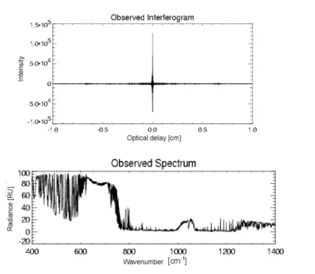
2.2.5 Example of downwelling atmospheric infrared measurement . . . 18
2.3 Weighting function . . . 20
2.4 The line-by-line radiative calculation . . . 21
2.5 Sensitivity study . . . 23 v
vi CONTENTS
3 Instrument and model data 27
3.1 AERI . . . 27
3.1.1 Instrument design . . . 28
3.1.2 Data acquisition . . . 29
3.2 Microwave radiometer . . . 32
3.3 GPS data . . . 33
3.4 Tower measurement . . . 34
3.5 COSMO DE model . . . 35
3.6 REMO model . . . 36
4 Quality control and evaluation of AERI data 39 4.1 Flagging low-quality data . . . 39
4.1.1 Imaginary part of observed radiances . . . 39
4.1.2 Instrument responsivity . . . 40
4.2 Finding clear sky cases . . . 40
4.3 Finding the best measured IWV and surface temperature to scale COSMO DE profiles 43 4.4 Spectral calibration . . . 47
4.5 Radiometric calibration . . . 49
4.5.1 Obstruction correction . . . 50
4.5.2 Aft optic correction . . . 52
5 Retrieval algorithm 55 5.1 Optimal Estimation theory . . . 56
5.2 The AERIoe . . . 58
6 CO2 profile retrieval for simulated radiances 63 6.1 CO2 retrieval with fixed temperature and humidity . . . 63
6.1.1 Retrieve the constant CO2 mixing ratio . . . 65
6.1.2 Parametrization of the CO2 profile . . . 67
6.1.3 Prior data of the three exponential function parameters . . . 69
6.1.4 Case studies . . . 72
6.1.5 Statistical assessment . . . 76
6.2 Simultaneous retrieval of CO2, temperature and humidity profiles . . . 79
6.2.1 The prior data of temperature and humidity profile . . . 79
6.2.2 Case studies . . . 80
6.2.3 Fixed surface CO2 concentration . . . 83
6.2.4 Noise filtering . . . 86
7 CO2 profile retrieval from real AERI measurements 91 7.1 Prior data of temperature and humidity profiles . . . 91 7.2 Simultaneous retrieval of temperature, humidity and CO2 profile . . . 93 7.2.1 Fixed the CO2 surface value . . . 109
8 Summary and outlook 113
Outlook . . . 116
Bibliography 119
Chapter 1
Introduction
Global warming, which is one of the main issues of the modern world, is a consequence of a rapid increase of atmospheric CO2 (Houghton, 2005). Analyzing the Greenland and Antarctic ice cores revealed a significant correlation between climate change and the increase in concentration of some atmospheric trace gases where CO2 was one of these trace gases (Delmas et al., 1980; Neftelet al., 1982). Therefore, during the last decades many studies focused on measuring and analyzing the atmospheric CO2 variation. Near the surface, the atmospheric CO2 concentration can have large diurnal variation due to interaction with the terrestrial ecosystem. Capturing this diurnal cycle can help characterize this interaction as one of the important parts of the natural carbon cycle. However, there is still a significant deficiency in the continuous measurement of the CO2 diurnal cycle in the boundary layer.
In the present study, we use continuous infrared measurements provided by a ground-based instrument to partially fill this gap.
1.1 Motivation
Thermal radiation emitted by the earth can be absorbed by several atmospheric trace gases such as H2O, CO2, O3, CH4 and N2O which causes an increase in the temperature of the troposphere. The troposphere then emits thermal radiation which can be absorbed by the earth. Absorption of thermal radiation by the earth increases the earth temperature and leads to further thermal emission by the earth. This cycle, which is known as greenhouse effect, causes a change in the mean surface temperature of our planet from -18 °C to 15
°C (Mitchell, 1989; Lorius et al., 1990; Mudge, 1997; Houghton, 2005). CO2 is the second most important atmospheric greenhouse gas after water vapor (Lorius et al., 1990; Houghton, 2005). However, the rapid increase of its emission due to human activities such as fossil fuel combustion and land use change makes it the most important anthropogenic greenhouse gas (IPCC, 1990). Since the industrial revolution at the beginning of 1750, 4000 million tons of anthropogenic carbon mainly in the form of CO2 along with substantial amounts of other trace gases such as CH4, N2O and chlorofluorocarbons (CFCs) have been released to the atmosphere annually (IPCC, 2013). As a result, the CO2 concentration in the atmosphere has increased by more than 40% since the industrial revolution (IPCC, 2013) and reached from 278 ppm (before 1750) to more than 400 ppm in 2016 (http://cdiac.ornl.gov/). If this growth rate continues during the 21st century, the CO2 content can reach the level that is the highest level in the past 20 million years (Houghton, 2005).
1
2 1. Introduction
The increase of the atmospheric CO2 content causes strong positive feedbacks such as an in- crease in the water vapor amount of the atmosphere (Manabe and Wetherald, 1967; Mitchell, 1989). The increment mainly of these two trace gases, H2O and CO2, enhances the absorp- tion of terrestrial radiation by the atmosphere. The consequence of this rise is an increase in the mean temperature of the earth surface as well as in the temperature of the atmo- sphere. The ice-core analysis in Vostok (East Antarctica) showed that there is a significant correlation (r=0.79) between atmospheric CO2 level and the change in the earth temperature (Barnola et al., 1987). The increase of the atmospheric CO2 and other trace gases also has some negative feedbacks such as the enhancement of low or middle clouds amount that can compensate the increase in the earth and atmosphere temperature (Charney et al., 1979).
However, several studies showed that the overall effect is a substantial warming (IPCC, 2001; IPCC, 2013). By using a radiative–convective model, Manabe and Wetherald (1967) predicted the climate sensitivity, which is defined as the change in the global mean equilibrium temperature of near surface as a result of doubling the atmospheric CO2, equals 2.2 K. Later in 1975, they derived an increase of 3 K using a three dimensional global circulation model (GCM). Further studies with more observational and reanalysis datasets support this overall substantial positive feedback and it was shown that the minimum increase is very unlikely to be below 1.5-2 K (Knutti et al., 2006). Finding an upper limit for climate sensitivity has been more challenging. Annan and Hargreaves (2006) proposed that the upper limit with very small probability (less than 5%) is more than 4.5 K. The range between 1.5 and 4.5 ◦C for the climate sensitivity is confirmed by other studies based on new observations and models during the last two decades. However, a small probability for an increase higher than 4.5 ◦C remains (Hegerl et al., 2006; Rogelj et al., 2012; IPCC, 2013; Mart´ınez-Bot´ıet al., 2015).
Accurate prediction of the future increase in global equilibrium temperature still suffers from different sources of uncertainty. One of them is the uncertainty in the carbon cycle mea- surement (Knutti et al., 2006). More accurate measurements of the atmospheric CO2 as the main carbon carrier in the atmosphere can substantially reduce this uncertainty. Sig- nificant progress in space-borne CO2 measurements in recent years has made considerable improvement in the accuracy of numerical model outputs. Besides, these measurements have also made a remarkable impact on providing a global view of carbon in the atmosphere (Ch´edin et al., 2002; Crevoisier et al., 2004; Buchwitz et al., 2005). However, satellite obser- vations are usually quite poor in capturing the diurnal cycle of CO2 in lower levels of the troposphere (Crevoisier et al., 2004; Morino et al., 2011). This problem can be solved by ground-based instruments since they can provide more accurate measurements in lower at- mospheric levels compared to satellites. The Total Carbon Column Observing Network (TC- CON) is a good example of a ground-based network implemented to produce accurate mea- surements for studying the carbon cycle as well as validation of satellites data (Wunch et al., 2011). However, because of using sunlight radiances for measuring the CO2, this network can only provide daytime measurements (Wunch et al., 2011) so that it does not have the abil- ity to capture the diurnal variation of the atmospheric CO2 profile. Terrestrial mechanisms such as photosynthesis and soil respiration as well as boundary layer processes can produce significant diurnal variation in the CO2 profile of lower tropospheric levels. Capturing this diurnal cycle which is important for studying the effect of the terrestrial ecosystem on the atmospheric CO2 profile is one of the main challenges for numerical models predicting the near surface CO2 flux (Tolk et al., 2009). Therefore, continuous CO2 measurements during daytime and nighttime are highly needed in order to improve these models and to validate their outputs as well as studying the CO2 diurnal variation and its effect on the carbon cycle.
The Fourier Transform InfraRed (FTIR) emission spectroscopy is a well-known method
1.2. Carbon cycle 3 of remote sensing in different fields. In atmospheric research, for the first time in 1969, an Infrared Radiation Interferometer Spectrometer (IRIS) was used on-board the Nimbus- 3 satellite (Conrath et al., 1970) and later an improved one used on-board the Nimbus-4 (Hanel et al., 1972). Afterwards, the request for more accurate measurements of atmospheric parameters lead to the design and installation of a new generation of FTIR spectrometers on-board several satellites (Smith et al., 1983, 1990a;Revercomb et al., 1988;Clerbaux et al., 2009). For ground-based atmospheric measurements, the FTIR spectroscopy is applied with roughly 20 years delay compared to satellite measurements (Smith et al., 1990b). Since then, several FTIR spectrometers have been developed and installed around the world in different fields of atmospheric research such boundary layer studies, climate research and cloud studies (Smith et al., 1993, 1999; Lubin, 1994; Sp¨ankuch et al., 1996;Feltz et al., 2003;
L¨ohnertet al., 2009;Turner and L¨ohnert, 2014). One of these FTIR instruments which were designed to measure the atmospheric thermal emission with high spectral and temporal reso- lution is the Atmospheric Emitted Radiance Interferometer (AERI) (Revercomb et al., 1994;
Knuteson et al., 2004a). The AERI is a ground-based instrument that measures downwelling atmospheric mid-infrared radiances continuously. It was designed and developed at the Uni- versity of Wisconsin-Madison (Knuteson et al., 2004a). The AERI measurements have shown high ability to retrieve atmospheric parameters such as temperature and humidity profile as well as cloud properties (e.g. L¨ohnertet al., 2009; Turner and L¨ohnert, 2014). Its obser- vations also showed sensitivity to the atmospheric CO2 content (Feldman et al., 2015). In 2011, an AERI instrument was installed at J¨ulich ObservatorY for Cloud Evolution (JOYCE) (L¨ohnert et al., 2015), Germany and it has provided measurements since 2012. Continuous measurements of the AERI during nighttime and daytime provide a great opportunity for studying the diurnal CO2 variation in the boundary layer. The aim of the present work is to use these highly spectrally and temporally resolving measurements to provide information about the CO2diurnal cycle in the lower atmosphere in order to partially improve deficiencies in carbon cycle studies.
This research has been supported by HITEC graduate school for energy and climate
(www.hitec-graduate-school.de). HITEC is a graduate school at the Forschungszentrum J¨ulich that supports the PhD students working on energy and climate research. It is a partner of different universities such as Universit¨at zu K¨oln, RWTH Aachen University and Heinrich-Heine-Universit¨at D¨usseldorf. The aim of HITEC is to provide an interdisciplinary communication between PhD students in order to enhance their scientific experiences as well as providing different opportunities to improve their professional skills and qualifications.
HITEC is funded by the Helmholtz Initiative and Networking.
1.2 Carbon cycle
Carbon does not have a natural sink; it can only flow between three natural reservoirs con- sisting of land (the biggest one), ocean and atmosphere (the smallest one). This natural cycle is called the global carbon cycle (IPCC, 1990). For several thousands of years, before the industrialization, the concentration of CO2 in the atmosphere was fluctuating roughly between 180 and 280 ppm (Petit et al., 1999; L¨uthi et al., 2008; H¨onisch et al., 2009). Since the industrial era around 1750, anthropogenic activities such as extracting fossil fuels from geological pools and burning them along with deforestation in large areas released around 240 ± 10 PgC (1 PgC = 1015 gC) anthropogenic carbon into the atmosphere (IPCC, 2013).
However, less than half of this amount remained in the atmosphere and the rest has been
4 1. Introduction
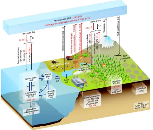
uptaken by two other reservoirs. This extra anthropogenic carbon emission increased the CO2 atmospheric concentration by more than 100 ppm (IPCC, 2013). Fig. 1.1 shows the global carbon cycle between the three natural reservoirs for the time period before and after the industrial revolution.
Carbon exchanges between atmosphere and other reservoirs can be divided into different classifications based on their time scale; carbon cycling from decade to centuries which can happen in the carbon exchange between plants, soils and the ocean surface with the at- mosphere; centuries to millennia for exchanging carbon between deeper soils and the deep ocean with the atmosphere; and up to millions of years for transferring carbon between the atmosphere and geological pools e.g. carbonate sediments in deep sea (IPCC, 2013).
The atmospheric CO2 is growing at about half of the rate of total CO2 anthropogenic emis- sions into the atmosphere. The other half is uptaken either by the terrestrial ecosystems or dissolves in the sea water surface and the deep ocean (IPCC, 2001). Therefore, any small change in these two reservoirs can have a considerable effect on the atmospheric CO2 con- tent within years to a decade. Consequently, it is essential to learn about these reservoirs and their mechanism for uptaking or emitting the CO2 in different conditions as well as the impact of the rapid increase of anthropogenic atmospheric carbon on them. In the next two subsections, these two reservoirs and their role in the global carbon cycle is briefly explained.
1.2.1 Terrestrial ecosystem
A terrestrial ecosystem can have different impacts on the atmospheric CO2 content. While plant photosynthesis during daytime produces a sink for atmospheric CO2, soil respiration and other oxidization processes such as decomposition or oxidation of organic materials generate a source of atmospheric CO2.
The total amount of CO2 uptaken by plants is known as gross primary production (GPP) (IPCC, 2001). The CO2interacts with water inside leaves and its oxygen isotope changes from
16O to 18O. Many of these CO2 molecules participate in photosynthesis process and diffuse out again which make them measurable in the atmosphere (Ciais et al., 1997). By measuring this CO2 type, the contribution of plants in the uptake of the atmospheric CO2 can be estimated. About half of the uptaken CO2 amount, known as net primary production (NPP) remains in the plants and is consumed for growing new plant tissues such as leaves, roots and woods; the rest returns to the atmosphere by plant tissue respiration (Lloyd and Farquhar, 1996; Waring et al., 1998). Ultimately, all the carbon which is used for growing plant tissues comes back to the atmospheric reservoir mainly by two processes; plant and soil respiration by bacteria, some fungi types and herbivores; and natural combustion or human-made fires (IPCC, 2001). The amount of carbon that is lost or gained by every ecosystem can be influenced by anthropogenic activities, perturbation in the natural ecosystem and climate variability (IPCC, 2001). However, currently, the terrestrial ecosystem acts as a global sink for atmospheric carbon (IPCC, 2013).
The growth of the human population and consequently the increase in the request for more food as well as wood products have caused deforestation in large areas and land use change mainly for growing more agricultural products. These activities have decreased the ability of the ecosystem for uptaking the atmospheric CO2. However, reforestation in Europe and North America has compensated this effect in recent years (IPCC, 2013). Some other im- portant anthropogenic factors which affect the amount of CO2 that can be uptaken by the
1.2. Carbon cycle 5
Figure 1.1: The carbon cycle between the 3 natural reservoirs, land, ocean and atmosphere.
Black numbers and arrows show the estimated carbon mass in each reservoir and annual ex- change fluxes between the three reservoirs for the time period before the industrial revolution.
Red arrows represent the mean annual anthropogenic fluxes over time period between 2000 and 2009. Red numbers indicate the cumulative change of carbon in each reservoir due to the anthropogenic activities over the 1750-2011 industrial period (taken from IPCC, 2013).
terrestrial ecosystem are fire, drastic grazing and draining peatlands or wetlands for agricul- tural purposes (IPCC, 2001).
A significant amount of carbon is transported from soil to water through several ways. Carbon can be buried in the organic sediment of freshwater or it can go to the coastal ocean through rivers while parts of it may outgas as CO2and back to the atmosphere (Tranvik et al., 2009).
In the next subsection, the role of the ocean as the second most important natural reservoir in the global carbon cycle is presented.
1.2.2 Ocean
Higher solubility and chemical reactivity of CO2compared to other anthropogenic gases such as CH4and CFCs allows for a more efficient uptake by sea water (IPCC, 2001). The exchange of CO2 between the ocean surface and the atmosphere can be shown as:
CO2+H2O+CO32−⇋2HCO−3, (1.1) where CO2−3 and HCO−3 indicate the carbonate ion and bicarbonate ion (IPCC, 2013). This flux known as “solubility pump” is mainly due to the CO2 partial pressure (pCO2) difference
6 1. Introduction
between ocean surface and the atmosphere as well as the solubility of CO2. The solubility by itself is a function of temperature and gas transfer coefficient (IPCC, 2001). The enhancement of the anthropogenic CO2in the atmosphere increases pCO2so that the uptake of atmospheric CO2 by the surface ocean rises which is a superimposed uptake on the global natural transfer (IPCC, 2001; IPCC, 2013). The dissolved CO2 in the ocean is known as Dissolved Inorganic Carbon (DIC). As Eq. 1.1 shows, the DIC is found in three main forms. The biggest part belongs to the bicarbonate ion (HCO−3, about 90%) where the carbonate ion (CO2−3 , about 8%) and the dissolved CO2 (non-ionic about 1%) are quite smaller parts (IPCC, 2001).
Another main source of carbon in the ocean is the Dissolved Organic Carbon (DOC) (IPCC, 2013). The DOC is a result of the gross primary production produced by phytoplanktons and other microorganisms in the ocean. The DOC together with dead organism and detritus transfer organic carbon vertically into the deeper ocean. Part of this production remains as the net primary production of the ocean (the main source of the DOC) while the other part is returned to the DIC through autotrophic respiration i.e. respiration by photosynthetic organisms. The sinking of a fraction of the DOC along with other particular organic carbon which is composed of dead organisms and detritus create a downward flux of organic carbon from upper ocean known as export production (IPCC, 2001). A very small fraction (less than 1%) of this export production remains in the ocean reservoir as sediments, mostly in the coastal ocean. The rest converts to the DIC. Without this mechanism which is known as biological pump, the atmospheric concentration would be about 200 ppm higher than its current concentration (Sarmiento and Toggweiler, 1984; Maier-Reimeret al., 1996).
Conceptually, the ocean has enough capacity to uptake more than 70 to 80% of anthro- pogenic atmospheric CO2. However, the solubility rate of CO2 in the ocean surface sets a considerable limit for this capacity meaning that the ocean needs several hundred years to reach this capacity (Maier-Reimer and Hasselmann, 1987; Enting et al., 1994; Archer et al., 1997). Since the atmosphere is the smallest reservoir of the carbon cycle, any slight change in the atmospheric carbon amount (particularly in the atmospheric CO2 as a main carbon barrier in the atmosphere) can cause a significant effect on the global carbon cycle. This indicates the importance of tracking the atmospheric CO2 content. Accurate measurements of the CO2 content in the atmosphere can help to properly estimate the effect of rising the human-emitted CO2 mainly on the future climate. In the next section the history of atmo- spheric CO2 measurements, as well as recently-used methods and instruments in this field, are presented.
1.3 Atmospheric CO
2measurement
Reliable prediction of future atmospheric CO2 concentration and its impact on the earth climate need accurate measurements of its mean atmospheric concentration as well as its diurnal, seasonal and annual cycles in the atmosphere. In this section different kinds of atmospheric CO2 measurements i.e. in-situ, space-based and ground-based measurements, together with their advantages and deficiencies, are introduced.
1.3.1 In situ measurements
Because of the long lifetime of the atmospheric CO2 (Archer et al., 1997), even a local mea- surement can represent approximately the CO2 global trend. There are many in situ mea- surements of CO2 around the world; the oldest one is the Mauna Loa observatory located in
1.3. Atmospheric CO2 measurement 7
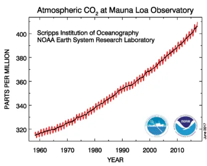
Figure 1.2: The CO2 volume mixing ratio measured at the Mauna Loa Station in Hawaii.
The data are presented from 1958 to June 2017 (taken from http://esrl.noaa.gov/gmd/).
the Hawaiian Islands (Keeling et al., 1976). The hourly collected air samples at the top of four 7-m towers are analyzed using a nondispersive infrared gas analyzer in order to determine the CO2 concentration. Fig. 1.2 shows the long term observation of the CO2 volume mixing ratio (VMR) provided by this site from 1958 to 2017. In addition to the seasonal cycle of CO2 which can be seen clearly in the plot, it shows the significant increase of atmospheric CO2 during last 60 years in a way that it reached up to 400 ppm in 2016.
In addition to the Mauna Loa station, the Scripps Institution of Oceanography (SIO) air sampling network has 11 observatory stations for recording the atmospheric CO2 which are distributed mainly on the Pacific Ocean (http://cdiac.ornl.gov). Furthermore, the In- Situ Measurement Program of the Global Monitoring Division (GMD), belonging to the National Oceanic and Atmospheric Administration (NOAA)’s Earth System Research Lab- oratory (ESRL), monitors several greenhouse gases including CO2 to analyze its short term and long term variations. These in situ measurements include 4 NOAA Baseline Observato- ries at Barrow, Mauna Loa, American Samoa and South Pole; and a tall tower network in US (e.g. Thoning et al., 1989; 2000; www.esrl.noaa.gov). These in-situ measurements mainly use the nondispersive infrared gas analyzer to determine the CO2 concentration of the col- lected air samples at the towers. Besides, there are also some long term CO2 observatory stations around the world such as the Amsterdam Island station that was located in the south Indian Ocean 5000 km off South Africa. It measured data from 1980 to 1995 (Gaudry et al., 1983, 1991; Lambert et al., 1995); The K-puszta air pollution monitoring station that was set in Hungarian Great Plain and provided CO2 measurements between 1981-1997 (Haszpra, 1995); The Jubany Station on King George Island, Antarctic belongs to the Italian PNRA (National Research Program in Antarctica) and performed continuous CO2 measurements recording from 1994 to 2009 (e.g.Ciattaglia et al., 1997) and the Baring Head station in New Zealand which provided data from 1970 to 1993 (e.g. Manning and Pohl, 1986).
In addition to the ground-based in-situ measurements, there are radiosonde-based in-situ
8 1. Introduction
instruments such as AirCore (Karion et al., 2010) which is a stainless steel tube and can evacuate while ascending in order to collect the air samples while its descending. Moreover, the aircraft-based in-situ measurements collected during flight campaigns are used to validate and evaluate other measurements (Wunch et al., 2010, Messerschmidt et al., 2011). As an example, a flight campaign in 2009 over Europe which was used for calibration of ground- based CO2 measurements (Messerschmidtet al., 2011).
1.3.2 Space-based measurements
Recent significant progress in satellite measurements had a considerable impact on the study of the chemical components of the earth atmosphere such as CO2and O3. The big advantage of satellite measurements is to provide a global view of the atmospheric CO2 which is a practical tool for studying CO2sinks and sources on the surface (Raven and Falkowski, 1999).
One of the first atmospheric CO2 concentration retrievals from a space-borne instrument belongs to the Television and InfraRed Operational Satellite-Next generation (TIROS-N) Operational Vertical Sounder (TOVS) that was flown on-board the NOAA polar meteoro- logical satellites (Ch´edin et al., 2002). Infrared and microwave observations from the High resolution Infrared Radiation Sounder (HIRS-2), the Microwave Sounding Unit (MSU) and the Stratospheric Sounding Unit (SSU) over the tropic [20S:20N] for the period of July 1987–
June 1991 were used for retrieving the monthly mean mid-tropospheric CO2 concentration.
The results show good agreement with the present knowledge of the seasonal and annual atmospheric cycles (Ch´edin et al., 2002, 2003).
In March 2002, the European Space Agency (ESA) launched the environmental satellite ENVISAT carrying the SCanning Imaging Absorption spectroMeter for Atmospheric CHar- tographY (SCIAMACHY) (Burrows et al., 1995, Bovensmann et al., 1999). SCIAMACHY measured the upwelling radiation in near-infrared region from 240 to 2400 nm. The de- rived dry air column averaged mixing ratios, XCO2 from clear sky measurements over land showed good agreement with global model data. In addition, for the first time, a regional source/sink map of CO2 on earth was detected from the space using the SCIAMACHY ob- servation (Buchwitz et al., 2005).
In addition, NASA’s Aqua satellite was also launched in May 2002. Thermal infrared ra- diation near the CO2 absorption line at 15 µm has been measured by the Atmospheric Infrared Sounder (AIRS) on-board this satellite. Due to the strong absorption of this band, the instrument could not get any information about the CO2 near surface layer. Therefore, the measurements are limited to the mid-tropospheric CO2 concentration between 5 and 7 km (Crevoisier et al., 2004). A global map of the CO2 amount in the upper troposphere at a resolution of 15◦×15◦ is derived from monthly measurements over cloud-free condition (Crevoisier et al., 2004; Chevallier et al., 2005).
The Greenhouse gases Observing SATellite (GOSAT, IBUKI in Japanese) is the first satellite dedicated to measuring greenhouse gases (Kuze et al., 2009). GOSAT was a joint project of Japan Aerospace Exploration Agency (JAXA), the National Institute for Environmental Science (NIES) and the Ministry of the Environment (MOE), which was launched on 23 January 2009 (Kuzeet al., 2009). One instrument on-board GOSAT is the Thermal And Near infrared Sensor for carbon Observation (TANSO) that is a Fourier Transform Spectrometer (FTS). The TANSO FTS uses a Michelson interferometer with two sets of detectors. It can observe the solar radiation reflected from the earth only during the daytime as well as atmospheric thermal radiation during both daytime and nighttime (Kuze et al., 2009). The
1.3. Atmospheric CO2 measurement 9 shortwave radiance have been used to get information about CO2 concentration near the earth surface while the thermal radiation has provided CO2 concentration mainly above 2 km (Saitoh et al., 2009). Only observations of clear sky condition can be applied for retrieving the column averaged amount, XCO2 (Saitoh et al., 2009). The first validation of its retrieved data was performed using measurements from a ground-based network. It showed a negative bias equal to 8.85±4.75 ppm for XCO2. However, both data showed similar CO2 seasonal cycle for the Northern Hemisphere (Morino et al., 2011).
Another satellite dedicated to studying atmospheric CO2is the Orbiting Carbon Observatory- 2 (OCO 2, the first one lost during the launch in 2009) which was designed to capture regional CO2 sinks and sources on the earth surface. The OCO 2 was launched on 2 July 2014. Its first data was sent on 6 September 2014 (Crispet al., 2017). Same as GOSAT, OCO 2 also measures reflected sunlight from the earth surface to retrieve the XCO2. Around 7 to 12 % of its monthly measurements belonging to cloud free conditions, have been used to derive the monthly mean value of XCO2 (Crisp et al., 2017). The analysis of its first 18 months of data revealed main features such as a considerable enhancement of XCO2 from October until December over the eastern US and eastern China due to the strong fossil fuel combustion as well as enhanced XCO2 in Amazon, central Africa and Indonesia because of biomass burning in this time period; a reduction of more than 10 ppm in the XCO2 of Northern Hemisphere in May and June (compared to other months of year) due to the plant photosynthesis and a significant north-south gradient of XCO2 in May and June (Eldering et al., 2017).
1.3.3 Ground-based measurements
Although satellite measurements can give a global view of the atmospheric CO2concentration, they are usually rather poor in capturing fine CO2 variations near the earth surface. Besides, high-precision independent datasets are needed for validation of space-borne measurements.
For these reasons, ground-base measurements are designed and developed. The Total Carbon Column Observing Network (TCCON) is one of the best example of the ground-based network which was established in 2004. The main purpose of this network is to provide accurate measurements of XCO2 (0.25% or less than 1 ppm precision) for studying the global and regional carbon cycle, for data assimilation studies and linking satellite measurements to ground based measurements (Wunch et al., 2011). Currently, there are 18 sites affiliated with TCCON where 15 of them are operational (Wunch et al., 2011). TCCON instruments use near infrared measurements with sensitivity to the atmospheric CO2. Two detectors cover the sensitivity of entire spectral region from 3900-15500 cm−1 which is the same spectral region used by different satellites particularly SCIAMACHY, GOSAT and OCO 2. As auxiliary measurements, accurate surface temperature and pressure measurements are used at each site (Wunch et al., 2011).
A comparison between Park Falls TCCON data with SCIAMACHY measurements in lower tropospheric levels showed the accuracy of SCIAMACHY for capturing the seasonal cycle of the XCO2 as a result of growing plants on monthly time scales (Barkley et al., 2007).
Furthermore, comparing retrieved CO2 column amounts from five European TCCON sites with CO2profiles derived from an aircraft campaign over these sites showed the suitability of TCCON data for calibration and validation of nadir viewing satellites (Messerschmidt et al., 2011).
The TCCON measurements are limited to daytime measurements therefore these data are useless for capturing diurnal variations of CO2 concentration particularly in lower atmo- spheric levels where these variations due to the plant photosynthesis and respiration as well
10 1. Introduction
as boundary layer mechanism can be quite significant. Thermal infrared radiation can be measured both in daytime and nighttime. The high spectral resolution measurements of ther- mal infrared radiation which have sensitivity to several atmospheric trace gases including CO2
can help to study the diurnal cycle of CO2near the earth surface. The Atmospheric Emitted Radiance Interferometer (AERI) is a ground-based instrument that measures the downwelling atmospheric thermal radiation from 520 cm−1(19µm) to 3020 cm−1 (3.3µm) with a spectral resolution of better than 1 cm−1 (Knutesonet al., 2004a). AERI was designed to improve and evaluate the line-by-line radiation codes as well as to retrieve boundary layer properties such as temperature and humidity profile (e.g. Revercomb et al., 2003; Turneret al., 2004).
Its highly temporally and spectrally resolving measurements have already been used for re- trieving the temperature and humidity profile (e.g. L¨ohnert et al., 2009). However, there are just a few studies about using its measurements for studying atmospheric trace gases. In the present work, the sensitivity of AERI measurements to the atmospheric CO2 is analyzed and is used to provide proper information about the diurnal variation of CO2 near the surface.
In the next section, the main goal of this study and the structure of the thesis are described.
1.4 Goal and structure of the thesis
The analysis of atmospheric CO2 variations mainly in the boundary layer is a great tool for studying the impact of the terrestrial ecosystem as well as sea-water on the atmospheric CO2concentration. However, capturing these variations needs accurate measurements during daytime and nighttime. Thermal infrared radiation which includes the 15 µm CO2 line and is measurable during daytime and nighttime has the potential to be used in this respect.
The main focus of the present work is to exploit these radiances in order to provide the atmospheric CO2variations in the boundary layer. This information can be used for studying land vegetation mechanisms such as photosynthesis and soil respiration. Such data are also valuable for the validation of different numerical models which predict the near surface CO2 flux.
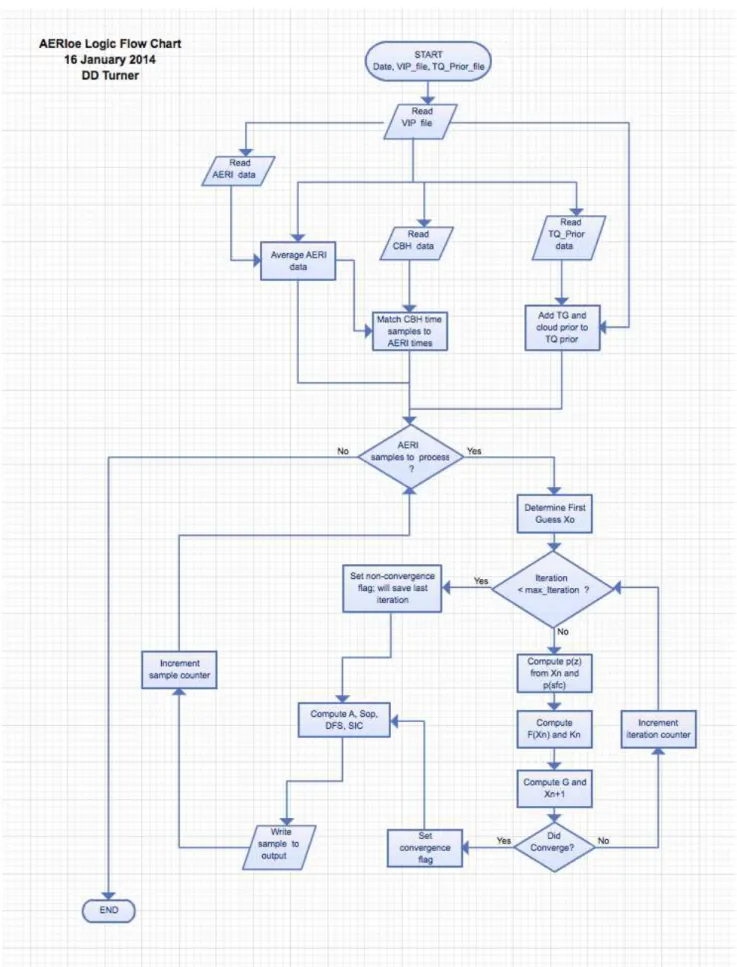
For this purpose, observations of the AERI instrument in 2012 at JOYCE are used. First the sensitivity of AERI radiances to the atmospheric CO2 profile is analyzed. Then an algorithm named AERIoe (Turner and L¨ohnert, 2014) is used to retrieve the CO2 profile in the boundary layer. The AERIoe is a variational retrieval algorithm which applies the optimal estimation method for retrieving the temperature and humidity profile. In the present study, the AERIoe is modified to retrieve the CO2 profile mainly in the boundary layer. In order to evaluate the theoretical potential of the algorithm in retrieving the atmospheric CO2 profile, the AERIoe is applied to simulated AERI radiances which are provided by an accurate line- by-line radiative transfer model. After that, the real calibrated measurements of the AERI in clear sky cases are used for retrieving the diurnal cycle of the CO2 concentration. Then retrieval results are compared with in-situ tower measurements in J¨ulich. In chapter 2, a general description of radiative transfer theory as well as short description of the line-by- line radiative transfer model LBLRTM are presented, followed by a section about studying the sensitivity of simulated AERI radiances to the variation of the atmospheric CO2 profile.
Different instruments as well as all measurements and data products related to this work are described in chapter 3. Chapter 4 deals with the calibration and the quality control of AERI measurements at JOYCE in 2012. The principal of optimal estimation method and the retrieval algorithm AERIoe which are used in the present work are given in chapter 5.
The modification of the AERIoe in order to retrieve the atmospheric CO2 profile is given in
1.4. Goal and structure of the thesis 11 chapter 6. Applying the simulated AERI radiances in the modified AERIoe as well as its results are also presented in this chapter. In chapter 7, real AERI observation radiances are used in the AERIoe and the results are compared with another observation provided by the tower mesurements at JOYCE. In addition, a discussion on some issues related to the real AERI observation radiances at JOYCE is given in this chapter. Finally, the summary of this study as well as the outlook for future work are presented in chapter 8.
Chapter 2
Radiative transfer
Electromagnetic radiation of the sun known as solar radiation consists of different wavelengths from gamma rays with wavelengths less than 0.01 nm to radio waves with wavelengths larger than 1 m. The maximum intensity of solar radiation occurs around 0.5 µm. In addition, earth and atmosphere also emit electromagnetic radiation called terrestrial radiation with its maximum intensity around 10 µm. According to the wavelength of the maximum inten- sity, solar radiation is named shortwave radiation while earth-atmosphere radiation is named longwave radiation.
Longwave radiation can be absorbed by several atmospheric trace gases such as H2O, CO2 and O3 due to the interaction between the electromagnetic radiation and these atmospheric trace gases. This interaction can be characterized by radiative transfer theory. The main focus of the present chapter is to shortly explain the Radiative Transfer Equation (RTE) specifically for the infrared region in clear sky conditions. In the first section, the basic RTE is derived. Then the possible solutions of this equation in the infrared region are investigated in section 2.2 followed by an overview of weighting functions that show the absorption weighting of a trace gas in terms of atmospheric altitude. In section 2.4, the line-by-line calculation of atmospheric radiation is explained and a pretty accurate numerical model for simulating atmospheric radiation is presented. Finally, in the last section, the sensitivity of thermal radiation to the change of CO2 content in the atmosphere is discussed. Detailed information can be found in many textbooks such as Petty (2006) and Liou (2002).
2.1 Basic radiative transfer in clear sky
The intensity of light (electromagnetic wave) may change along a path through a medium.
This change is due to the absorption or scattering of the light by different elements of the medium and can be characterized by the extinction coefficient βe.
βe=βa+βs, (2.1)
whereβaandβsrefer to the absorption and the scattering coefficients respectively. These two coefficients βa and βs mainly depend on the wavelength as well as physical medium. While scattering by a particle can be negligible for a specific wavelength in a specific medium, it can be very significant for another wavelength in the same medium. The single scatter albedo
13
14 2. Radiative transfer
˜
w is a ratio that shows the relative importance of scattering compared to absorption in a defined medium.
˜ w= βs
βe = βs
βs+βa. (2.2)
When this ratio goes to 0, scattering is negligible. Conversely, for a purely scattering medium, this ratio goes to 1. From now on, all equations in this chapter are obtained for the non- scattering atmosphere where ˜w and βs are negligible. In the next section, it is shown that why this assumption is valid for the present work.
For the clear sky atmosphere, absorption coefficients of several trace gases need to be consid- ered. Therefore, the total atmospheric gas absorption can be written as a sum of each trace gas absorption:
βa=X
i
βa,i. (2.3)
In addition, the absorption coefficient can be written in terms of mass absorption coefficient ka:
βa =ρka, (2.4)
where ρ shows the density of each trace gas. Consequently, we have:
βa=X
i
βa,i=X
i
ρika,i. (2.5)
When the light passes through a medium with the extinction coefficient of βa, its depletion along a path ds can be written as:
dIλ =Iλ(s+ds)−Iλ(s) =−Iλ(s)βa(s)ds, (2.6) where sshows the geometric distance between two points, I indicates the intensity of light and λ refers to the wavelength of the light. Note that I is considered as monochromatic meaning that it has a single wavelength. By integrating this equation froms1 tos2, we have:
Iλ(s2) =Iλ(s1) exp[−
Z s2
s1
βa(s)ds]. (2.7)
The term in the bracket is a dimensionless parameter which is called optical path τ: τ =
Z s2
s1
βa(s)ds. (2.8)
If the path is considered as a vertical distance, this term is known as optical depth or optical thickness and can be used as a vertical coordinate in the radiative application. Another useful parameter is transmittance twhich is defined by:
t(s1, s2) = exp[−τ(s1, s2)]. (2.9) Eq. (2.7) can be reformulated with this new parameter:
Iλ(s2) =t(s1, s2)Iλ(s1). (2.10) Another important interaction for radiative transfer is emission. Based on the Kirchhoff law, in the local thermodynamic equilibrium, the absorption of a specific matter is equal to its emission:
dIabs =−βa(s)Iλds=−dIemit=−βa(s)Bλ(T)ds, (2.11)
2.2. Radiative transfer in the infrared region for clear sky condition 15 where Bλ(T) shows the Planck function for a specific wavelength and temperature. This function gives the electromagnetic emission of a blackbody at a given temperature T in the thermal equilibrium. A blackbody is considered as a theoretically perfect absorber of all electromagnetic radiation which has no reflect on.
In general, for a non-scattering medium, the change in the radiation intensity can be written as:
dIλ =dIabs,λ+dIemit,λ=βa(s)(Bλ(T)−Iλ)ds, (2.12)
or dIλ
ds =βa(s)(Bλ(T)−Iλ). (2.13)
Eq. 2.13 is called Schwarzschild’s equation. This equation is the basic form of the radiative transfer equation (RTE).
The real atmosphere is often considered as a plane parallel atmosphere. The plane parallel atmosphere is an atmosphere whose parameters vary in the vertical direction, while these pa- rameters in the horizontal direction are assumed to be homogeneous. Therefore the variation in the zdirection, dz, can be used instead of dsand thus we have:
ds= dz cosθ = dz
µ, (2.14)
where θ is the zenith angle between the z and the sdirection andµ=cosθ. Substitution of Eq. (2.14) in Eq. (2.13) and using the mass absorption coefficient ka gives:
−µdIλ(z, µ)
kaρdz =Iλ(z, µ)−Bλ(T(z)). (2.15) In the next section, possible solutions of this equation in the infrared region are investigated.
2.2 Radiative transfer in the infrared region for clear sky con- dition
In the previous section, the RTE for the non-scattering plane-parallel atmosphere has been derived. This equation is well-suited for the thermal infrared region in the clear sky since the scattering of air molecules or aerosols, i.e. the only particles in a non-cloudy atmosphere, is negligible in the thermal infrared region. Therefore, the RTE can be characterized by two interactions, absorption and emission. For solving Eq. (2.15), two boundary conditions need to be defined. In a clear sky condition, the surface and the top of the atmosphere (TOA) can be considered as two appropriate boundaries. Note that the earth surface acts like a black body for the thermal infrared radiation and thus Iλ(surf ace)=Bλ(Tsurf ace). Besides, the total optical depth of the atmosphere needs to be calculated. The optical depth for a certain wavelength τλ can be calculated as:
τλ = Z z∞
z
kaλ(z′)ρ(z′)dz′. (2.16) Rewriting the Eq. (2.15) with τ gives:
µdIλ(τ, µ)
dτ =Iλ(τ, µ)−Bλ(T(τ)). (2.17)
16 2. Radiative transfer
Solving this equation gives the upward and downward components of the atmospheric radi- ation.
Iλ↑(τ, µ) =Bλ(T(τ∗))e
−(τ∗ −τ)
µ +
Z τ∗ τ
Bλ(T(τ′))e−(τ′−τ) µ
dτ′
µ , (2.18)
Iλ↓(τ,−µ) = Z τ
0
Bλ(T(τ′))e−(τ −τ′) µ
dτ′
µ , (2.19)
whereBλ(T(τ∗)) in Eq. (2.18) shows the emission from the earth. For the downward radiation, the emission from the TOA is Bλ(T OA) = 0. With these considerations, in Eq. (2.18), the first term shows the emission from the earth surface multiplied by the transmittance between the earth and an arbitrary altitude above it (shown by τ) which represents the attenuated emitted radiation of the earth surface. The second term in this equation is the integrated emission from each point between the earth and the arbitrary altitude. The downward radiation shown in Eq. (2.19) can be interpreted same as the upward radiation. The derived term in this equation shows the integrated emission between TOA and an arbitrary altitude below it (shown by τ).
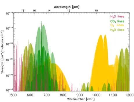
The most important atmospheric trace gases which lead to absorption and emission in the infrared region are H2O, CO2 and O3. The energy that is absorbed by a trace gas molecule can change into the different types of molecular energy such as translational kinetic energy, rotational kinetic energy, vibrational energy or it can change its electrical charge distribution.
While the translational kinetic energy of a molecule can have any continuous amount, the values of other three types of molecular energy are quantized. The quantized energy level means that the molecule can not have any arbitrary amount of energy and thus the energy levels are discrete such as E0, E1, ..., En. The electromagnetic radiation is also quantized.
The quantized unit of electromagnetic energy is called photon. Based on quantum mechanics, the energy E of a single photon is proportional to its wavelength/frequency.
E= hc
λ =hν, (2.20)
wherehis the Planck constant andcshows the speed of light;νandλrefer to wavelength and frequency of the photon respectively. A molecule can absorb/emit a photon, if the energy of the photon changes its molecular energy from one of its allowed state to another one meaning that only absorption/emission of a specified wavelength/frequency is allowed by a molecule.
Before reviewing the absorption/emission lines of atmospheric trace gases in the thermal infrared region, some fundamental concepts and definitions related to this topic are shortly summarized.
2.2.1 Vibrational and rotational transition
While the energy related to the microwave and far-infrared spectral bands can only change the rotational energy levels of a molecule and is too low for changing the molecular vibrational energy, the mid-infrared and near-infrared spectral region can change both the rotational and vibrational energy levels of a molecule. For changing the molecular electrical energy levels, higher frequency or lower wavelength such as visible or UV bands are needed. The focus of this section is on the thermal infrared or mid-infrared region and the different types of the molecular energy transition related to this region.
A pure vibrational transition is a transition from one allowed vibrational level to another one. The spectral band related to the pure vibrational transition is called Q branch. For
2.2. Radiative transfer in the infrared region for clear sky condition 17 example, a linear triatomic molecule such as CO2 has three different types of vibrational modes consisting of ν1, ν2 and ν3 corresponding to the symmetric stretch, bending and asymmetric stretch respectively. However, in reality, the vibrational and rotational transition may happen together. Consequently, the rotational levels which are shown by quantum number J can split the vibrational levels into finer ones. The Q branch is related to the
∆J = 0 and the spectral bands corresponding to ∆J =−1 and ∆J = +1 are called P and R branch respectively. The P and R branches present the vibrational-rotational transitions that are related to the emission or absorption lines slightly lower/higher than a pure vibrational line.
2.2.2 Line broadening
From the previous explanation given in section 2.2.1, one might assume that the absorption or emission lines have an exact frequency and thus should have a zero line width. However, in reality, they have a finite width. There are several reasons behind this physical phenomenon.
Some important ones, i.e. natural, pressure and Doppler broadening are summarized in the following.
The Heisenberg uncertainty principal is the fundamental reason for the line width which is called natural broadening. However, compared to other reasons, natural broadening is relatively small. In addition, in the troposphere and stratosphere with higher pressure and thus higher density of air molecules compared to the upper atmosphere, collision between air molecules disturb the basic absorption/emission molecular lines which is called pressure broadening. In the upper atmospheric levels such as the mesosphere and above it where the air molecules can move without restriction, the Doppler broadening is more significant.
The Doppler effect due to the speed of air molecules can cause the Doppler-shift in the absorption/emission wavelength of the molecules.
2.2.3 Continuum absorption
As it is mentioned in the previous subsection, in reality an absorption/emission line has a fi- nite width meaning that the line needs to be characterized with a line shape. The Lorentz line shape is the one which is used widely. This line shape is derived based on the instantaneous interaction between two molecules. This assumption agrees well for the weak interaction;
however, the close-range interaction deviates significantly from the Lorentz shape. For sim- plicity, an absorption/emission line is separated into two contribution, local line contribution and continuum contribution. The local line contribution can be considered as the spectral absorption up to some fixed distance from the line center (typically 25 cm−1) and any de- viation from the Lorentz shape within the line cutoff considered as continuum absorption (Turner and Mlawer, 2010).
The most important continuum absorption in the troposphere is water vapor continuum.
Although there is not any strong absorption line in 800 to 1200 cm−1, due to the water vapor continuum absorption, there is considerable thermal energy in this region. It has been shown that the optical depth of water vapor continuum absorption in this region varies with the square of the atmospheric water vapor amount which implies that these continuum bands are due to the interaction of two water vapor molecules known as “self-continuum”.
In addition, the interaction of water vapor molecules with different types of molecules can produce the continuum absorption known as foreign water vapor continuum. Clough et al.