Dynamics of Stone Habitats in Coastal Waters of the Southwestern Baltic Sea (Hohwacht Bay)

(1)

geosciences

Article

Dynamics of Stone Habitats in Coastal Waters of the Southwestern Baltic Sea (Hohwacht Bay)

Gitta Ann von Rönn^1,*, Knut Krämer¹, Markus Franz², Klaus Schwarzer¹ , Hans-Christian Reimers³ and Christian Winter¹

Citation: von Rönn, G.A.;

Krämer, K.; Franz, M.; Schwarzer, K.;

Reimers, H.-C.; Winter, C. Dynamics of Stone Habitats in Coastal Waters of the Southwestern Baltic Sea (Hohwacht Bay).Geosciences2021,11, 171. https://doi.org/10.3390/

geosciences11040171

Academic Editors: Vincent Lecours and Jesus Martinez-Frias

Received: 2 March 2021 Accepted: 7 April 2021 Published: 9 April 2021

Publisher’s Note:MDPI stays neutral with regard to jurisdictional claims in published maps and institutional affil- iations.

Licensee MDPI, Basel, Switzerland.

This article is an open access article distributed under the terms and conditions of the Creative Commons Attribution (CC BY) license (https://

creativecommons.org/licenses/by/

4.0/).

1 Institute of Geosciences, Coastal Geology and Sedimentology, Kiel University, 24118 Kiel, Germany;

knut.kraemer@ifg.uni-kiel.de (K.K.); klaus.schwarzer@ifg.uni-kiel.de (K.S.);

christian.winter@ifg.uni-kiel.de (C.W.)

2 GEOMAR Helmholtz Centre for Ocean Research Kiel, 24105 Kiel, Germany; markusfranz2707@gmx.de

3 State Agency for Agriculture, Environment and Rural Areas (LLUR), 24220 Flintbek, Germany;

hans-christian.reimers@llur.landsh.de

* Correspondence: gitta.vonroenn@ifg.uni-kiel.de

Abstract: Cobbles and boulders on the seafloor are of high ecological value in their function as habitats for a variety of benthic species, contributing to biodiversity and productivity in marine environments. We investigate the origin, physical shape, and structure of habitat-forming cobbles and boulders and reflect on their dynamics in coastal environments of the southwestern Baltic Sea. Stone habitats are not limited to lag deposits and cannot be sufficiently described as static environments, as different dynamic processes lead to changes within the physical habitat structure and create new habitats in spatially disparate areas. Dynamic processes such as (a) ongoing exposure of cobbles and boulders from glacial till, (b) continuous overturning of cobbles, and (c) the migration of cobbles need to be considered. A distinction between allochthonous and autochthonous habitats is suggested. The genesis of sediment types indicates that stone habitats are restricted to their source (glacial till), but hydrodynamic processes induce a redistribution of individual cobbles, leading to the development of new coastal habitats. Thus, coastal stone habitats need to be regarded as dynamic and are changing on a large bandwidth of timescales. In general, wave-induced processes changing the physical structure of these habitats do not occur separately but rather act simultaneously, leading to a dynamic type of habitat.

Keywords: stone habitat; dynamic habitat; habitat mapping; hard-bottom communities;

coastal evolution; Baltic Sea; shallow water

1. Introduction

Hard substrates are important geo-habitats in marine environments and function as vital contributors to coastal biodiversity [1–3]. In addition to rocky surfaces, essential features are stones, boulders, and blocks, which are here termed as cobbles and boulders, following the Kolp classification [4]. Cobble and boulder assemblages show high structural complexity and heterogeneity, which facilitate coexistence and higher biodiversity by increasing the availability of microhabitats and shelter from predation [5–7]. Additionally, these habitats provide feeding grounds for fish, birds, and marine mammals and serve as spawning and nursery areas for many fish species [8–10]. In the Baltic Sea, they belong to those habitats with the most diverse community types, providing various ecosystem services [11,12]. Conservation, protection, and suitable management of these environments require precise knowledge about their occurrence, structure and spatial diversity, their status, and their environmental conditions [13,14]. This system knowledge also in- forms reporting to guidelines such as the Marine Strategy Framework Directive (MSFD, 2008/56/EC) [15] and the Habitat Directive (HD 92/43/EEC annex 1 1170-reefs) [16,17].

Geosciences2021,11, 171. https://doi.org/10.3390/geosciences11040171 https://www.mdpi.com/journal/geosciences

(2)

Geosciences2021,11, 171 2 of 18

Coastal habitats are increasingly affected by human activities such as fishing, urban- ization, marine traffic, extraction of mineral resources, tourist industry, eutrophication, and coastal development [18,19]. From about 1800–1976, boulders have been extracted for commercial purposes from shallow water areas of the southwestern Baltic Sea [20,21].

This changed the sedimentological and geomorphological structure and the ecological conditions within these environments substantially [20,21]. However, some boulders have been left and since the ban of boulder extraction in 1976, their number is increasing again due to ongoing erosion and exposure of new cobbles and boulders from the glacial till [22].

Marine cobble and boulder habitats (stone habitats hereafter) within the southwestern Baltic Sea are mostly composed of cobbles (Ø 6.3–63 cm) and boulders (Ø 63–630 cm) on the otherwise sandy or cohesive consolidated seafloor [4]. The origin of these large clastic elements are glacial till deposits, in water depths from 0 down to about−20 m [22,23].

Therefore, in previous studies, it has been assumed that the occurrence of stone habitats is necessarily connected to lag deposits composed of coarse sand, gravel, cobbles, and boulders [24–26].

For several decades, cobbles and boulders on abrasion platforms have been considered to be immobile [27–29]; however, Schrottke et al. (2006) showed high mobility of gravel and small cobbles in field experiments [30]. Yet, little is known about the effects on habitats.

The sizes of cobbles and boulders, their spatial distribution and extent, the overturning of cobbles and boulders, and their transport have rarely been discussed in earlier studies.

In addition, information from shallow water environments (0–10 m water depth) is scarce since they are often influenced by strong waves impeding field surveys. Few studies concerning stone habitats in shallow waters exist, e.g., from the Mediterranean Sea in water depths between 15–20 m, where it was shown that instability of rocky substrates and their lithology can influence colonization [31]. Diverse studies on benthic community structure indicate a strong correlation between biodiversity and physical habitat structure [32–35], which can be assumed to be pronounced in the most dynamic shallow water environments.

Several studies on hard substrates reveal physical disturbance as one of the primary forces influencing species diversity [36–38]. Overturning, as a physical process acting on cobbles, destroys macroalgae on the substratum surfaces and results in opportunities for new organisms to settle [36,39].

Shallow water habitats are a particularly dynamic environment and seafloor changes depend on the timescales being considered. Wind-generated waves and resulting currents are the dominating hydrodynamic forces in the southwestern Baltic Sea. They have a high impact on seafloor morphology and sedimentology [40]. Physical and sedimentological processes can disturb benthic ecosystems, e.g., by sediment mobilization during storms when benthos is unable to remain attached or is buried under rapidly deposited sediments [41].

Our understanding of stone habitats in coastal environments is fragmentary as it originates from temporarily scattered observations. Additionally, investigations often lack spatial resolution to assess the habitat state. In this study, we investigated two stone habitats in Hohwacht Bay (SW Baltic Sea, Figure1) to characterize the size and shape of individual cobbles and boulders and their spatial distribution. Additionally, we analyzed the benthic community structure of single cobbles and boulders. We explain differences between physical structures of the stone habitats and describe different modes of stone habitat dynamics: (a) the formation and extension of the habitat through cobble and boulder exposure, (b) the development of new settlement space by overturning of cobbles, and (c) the creation of new habitats by the migration of cobbles.

(3)

Geosciences 2021, 11, x FOR PEER REVIEW 3 of 18

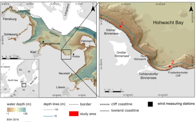
Figure 1. Bathymetric map of the southwestern Baltic Sea including the study areas (Bathymetric data provided by BSH (www.geoseaportal.de) (Accessed on: 20 August 2019).

2. Regional Setting

The seabed of Hohwacht Bay, located in the southwestern Baltic Sea (Figure 1), is mainly composed of glacial till deposited and consolidated during the last glaciation. Dur- ing the Holocene, the postglacial coastal landscape was flooded since the Littorina transgression, which began about 8.000 BP (Before Present) [42,43]. Since then, dynamic processes induced by waves and currents have constantly shaped the coastal environment by erosion, sediment transport, and deposition [23,43]. The initially strongly lobed coastlines, which were left after the deglaciation, have been smoothed: Protruding cliff sections were eroded and the sediments were transported and deposited alongshore, forming lagoons, freshwater lakes, and the so-called Bodden in Mecklenburg-Vorpommern. These freshwater lacustrine environments are separated from the open sea by beaches and beach ridges [23,44,45], and thus, organic-rich, fine-grained sediments known as gyttja or mudde are deposited under low-energy conditions [46–48].

Due to sea-level rise, earlier lagoons and lakes have been flooded by further transgression. The coast is retreating, and thus, lacustrine sediments, deposited in lakes or lagoons in the past, are cropping out in the shallow waters offshore the coastal lowlands today [45,48,49]. Contrastingly, in front of coastal cliffs, mostly between 0 and 20 m water depth, lag deposits composed of coarse sand, gravel, cobbles, and boulders cover the glacial till [23]. Typically, cobbles and boulders are distributed randomly within the lag deposits [22].

Two study areas, each with a size of 20 × 20 m, within the inner Hohwacht Bay were investigated—Study area 1 (SA1) is located in 3.5 m water depth, and 200 m offshore a coastal lowland and the freshwater lake “Kleiner Binnensee” (Figure 1). SA1 is primarily exposed to waves from northwesterly to easterly directions. The seafloor and its sur- roundings have been described as a large strip of gyttja, 400 m wide and extending parallel to the coast over 3 km [45]. This gyttja is completely exposed over wide areas and occasionally overgrown, either by eelgrass or covered by a thin layer of gravel. Landwards, it is bordered by mobile sand layers, seawards flanked by peat, which is followed seawards by glacial till. Study area 2 (SA2) is located 280 m offshore the Friederikenhofer Figure 1.Bathymetric map of the southwestern Baltic Sea including the study areas (Bathymetric data provided by BSH (www.geoseaportal.de) (Accessed on: 20 August 2019).

2. Regional Setting

The seabed of Hohwacht Bay, located in the southwestern Baltic Sea (Figure 1), is mainly composed of glacial till deposited and consolidated during the last glaciation.

During the Holocene, the postglacial coastal landscape was flooded since the Littorina transgression, which began about 8.000 BP (Before Present) [42,43]. Since then, dynamic processes induced by waves and currents have constantly shaped the coastal environment by erosion, sediment transport, and deposition [23,43]. The initially strongly lobed coastlines, which were left after the deglaciation, have been smoothed: Protruding cliff sections were eroded and the sediments were transported and deposited alongshore, forming lagoons, freshwater lakes, and the so-called Bodden in Mecklenburg-Vorpommern. These freshwater lacustrine environments are separated from the open sea by beaches and beach ridges [23,44,45], and thus, organic-rich, fine-grained sediments known as gyttja or mudde are deposited under low-energy conditions [46–48].

Due to sea-level rise, earlier lagoons and lakes have been flooded by further transgression. The coast is retreating, and thus, lacustrine sediments, deposited in lakes or lagoons in the past, are cropping out in the shallow waters offshore the coastal lowlands today [45,48,49]. Contrastingly, in front of coastal cliffs, mostly between 0 and 20 m water depth, lag deposits composed of coarse sand, gravel, cobbles, and boulders cover the glacial till [23]. Typically, cobbles and boulders are distributed randomly within the lag deposits [22].

Two study areas, each with a size of 20×20 m, within the inner Hohwacht Bay were investigated—Study area 1 (SA1) is located in 3.5 m water depth, and 200 m offshore a coastal lowland and the freshwater lake “Kleiner Binnensee” (Figure1). SA1 is primarily exposed to waves from northwesterly to easterly directions. The seafloor and its surround- ings have been described as a large strip of gyttja, 400 m wide and extending parallel to the coast over 3 km [45]. This gyttja is completely exposed over wide areas and occasionally overgrown, either by eelgrass or covered by a thin layer of gravel. Landwards, it is bordered by mobile sand layers, seawards flanked by peat, which is followed seawards by

(4)

glacial till. Study area 2 (SA2) is located 280 m offshore the Friederikenhofer Cliff (Figure1).

The water depth ranges from 5.5 m in its southern part to 6.3 m in its northern part. It is exposed to northwesterly to northeasterly directions. SA2 has been described as a part of a lag sediment deposit, which is the seaward extension of the cliff [50]. Mobile sand layers cover the seafloor landwards while lag sediment deposits extend seawards over the glacial till.

3. Materials and Methods 3.1. Area of Investigation

The seafloor of Hohwacht Bay (190 km²) was surveyed to identify areas with cobble and boulder assemblages and to distinguish sedimentological zones. Within the investigation area, two small-scale SAs were selected for a detailed analysis of the dynamics and functions of the occurring stone habitats (Figure1and Figure S1a–c). The selection was based on the differing geological prerequisites (offshore coastal cliff and offshore coastal lowland), geological units surrounding the stone habitats (lagoonal facies and glacial facies), and differences in water depth and exposition to wind and wave influence.

3.2. Hydroacoustic Surveys

Hydroacoustic surveys have been carried out in the investigation region to characterize the seafloor on a larger scale. Two cruises have been carried out with R/V Littorina in 2015 and 2016, surveying the seafloor between 5 and 18 m water depth. A towed side-scan sonar (SSS, Teledyne Benthos 1624) was used to collect full coverage acoustic backscatter information (Table1). Navigation data were obtained using the shipboard DGPS.

Within the shallow water (0.6–5 m water depth) a rubber boat was used to collect hydroacoustic data with a small-scale SSS (Tritech StarFish 452F) (Table1). Navigation data were recorded using an RTK–DGPS (GNSS 1200 +; Leica), combined with a heading sensor (Garmin Airmar).

Table 1.Survey Specifications.

Research Vessel.

Water

Depth (m) SSS Frequency (kHz)

Survey Speed (ms⁻¹)

Range (m)

Spatial Resolution (cm)

Littorina 5–18 Benthos

1624 400 2.3 100 20

Rubber

Boat 0.6–5 StarFish 452 2.3 80 20

Standard postprocessing was performed using geometric and radiometric correc- tions [51–53] in SonarWiz 7.03 [54]. Areas with high backscatter intensities are displayed in darker gray levels, while low backscatter intensities are shown in brighter gray levels (Figure S1a–c). Cobbles and boulders can be detected by their local high backscatter intensities due to the strong reflection of the acoustic signal, combined with their characteristic acoustic shadow [51,52,55]. ArcMap 10.6 (Esri) was used to manually create polygons around areas where cobbles and boulders occur. Areas were manually segmented, sepa- rating different seabed textures and backscatter areas, and were further classified using ground-truthing information from grab samples and underwater video observations.

3.3. Sediment Samples

Sediment samples to validate the SSS backscatter data were collected using a Van- Veen grab sampler (ship based) and by scientific scuba divers at SA1 and SA2. Grain size distributions of samples mainly composed of sand and fine gravel were obtained by mechanical sieving, using ¹₄PHI intervals according to the ASTM mesh standard [56].

Statistical parameters from the grain size distribution were determined using the software GRADISTAT [57]. Grain sizes were classified using the scheme of Kolp [4]. The sediment distribution map was not rigorously defined in grain size classes but categorized into four

(5)

sediment types, namely, lag sediments (sand–gravel), sand, fine-grained sediments (silt, clay), and gyttja (compacted, organogenic fine-grained sediments).

3.4. Size and Roundness of Individual Cobbles and Boulders

In this study, the term “stones” is used to describe solid geogenic hard substrates with grain sizes larger than 1 cm. Habitats composed of stones are referred to as “stone habitats,” accordingly. The Kolp scheme [4] was applied to further differentiate stones using the specific sedimentological terms “cobbles” (1–63 cm) and “boulders” (63–630 cm).

The Kolp classification was preferred over the Udden–Wentworth scale [58,59] and the in- ternational standard ISO 14688-1 [60] since it provides subclasses (small, medium, large;

Table2). The size class boundaries vary between the three different scales, which should be noted when relating the results of this study to others.

Table 2.Size Classification According to the Kolp Scheme.

Size Class Diameter (cm) Size Class Diameter (cm)

small cobble 1–6.3 small boulder 63–100

medium cobble 6.3–20 medium boulder 100–200

large cobble 20–63 large boulder 200–630

The physical habitat classifiers “habitat structure of hard-substrate areas” [34] or

“physical reef structure” [61] describe the abiotic components of stone habitats. Parameters characterizing the physical structure of stone habitats comprise the number of cobbles and boulders, their size, their form, their spatial distribution, and the type of their surrounding sediments. Here, divers performed in situ investigations within SA1 and SA2 including underwater video and image observations and sediment sampling. Within both study areas, all three axes (longest, medium, shortest) of cobbles and boulders, bigger than 10 cm in diameter, were measured to determine their size. For size classification in centimeters, the largest diameter was chosen.

For calculating the roundness of each cobble or boulder, the Corey shape factor (CSF) was used [62] as follows:

CSF= √^c

a∗b {CSF|0≤CSF≤1} (1)

witha= longest axis,b= medium axis, andc= shortest axis.

TheCSFdescribes the ratio of the cross-sectional area of a sphere to the maximum cross-sectional area of an ellipsoid, with the smallest value of theCSFdescribing the flattest form of the particle (Equation (1)) [62].

3.5. Wave Data

For local wave measurements, a pressure sensor (Driesen und Kern, MikroLog2-PT- S-STD-05) was deployed, and data were collected with a frequency of 2 Hz at SA1 in a water depth of 3.5 m. Since battery changes had to be conducted every two weeks and due to rough weather conditions, measurements were carried out in three periods: 14–26 March 2018, 4–16 April 2018, and 20 April–2 May 2018. For the period from 26 March to 7 May 2018, wave characteristics were calculated from pressure transducer data using the MATLAB functions by U. Neumeier [63]. The waves are described by significant wave height (HS) and maximum wave height (Hmax).

To extrapolate wave conditions for longer temporal periods, significant waves heights were calculated using the empirical shallow water forecasting equation (see below) in the Shore Protection Manual (SPM 84) [64] based on Bretschneider [65], which utilizes fetch length, water depth, and wind velocity (Equation (2)). Wind velocity and direction were obtained from the German Weather Service every 10 min [66]. Fetch length and average water depths, along with the profiles, were extracted from bathymetry [67] in 10^◦classes, corresponding with

(6)

the classes of wind directions from the DWD data. To achieve a good fit, the fetch was limited to Fmax= 20 km. The measured wave data were used to verify the recalculated wave heights.

gH_S,calc.

U²_A = 0.283tanh



0.530 gd U_A²

!3/4

tanh











0.00565 gF

U²_A

1/2

tanh

"

0.530 gd

U²_A

3/4#











(2)

whereg= gravitational acceleration [m/s²],H= wave height [m],UA= wind stress factor, d= water depth [m],F= fetch length [m],u= wind velocity [m/s].

To generate an average probability distribution of local significant wave heights (HS,calc.), a long-term record of hourly wind data was used (1 January 2010–31 December 2019) [66]

using Equation (2). To prevent multiple counting of single events, calculated wave heights were smoothed over a six-hour interval. The wind data were also used to calculate average wind directions and wind velocities. Since no wind measuring station is directly located at the SA1, wind data were interpolated by inverse distance weighting (IDW) between the stations Kiel Lighthouse and Putlos (for locations see Figure1).

3.6. Biological Sampling and Statistical Analysis

Hard-bottom communities associated with cobbles and boulders were sampled in May 2016. In each study area, divers collected biological samples. In SA1, five cobbles, and in SA2, six cobbles and boulders were randomly selected for sampling. The diameters of these cobbles and boulders ranged from 36 to 45 cm (SA1) and from 35 to 216 cm (SA2). For sample collection, a sampling frame (25 ×25 cm) was centrally positioned above a cobble or boulder and all contained biota were scraped off. The collected material was directly transferred into zipper bags and within the following three hours, fixed in a buffered formaldehyde solution (final concentration of 4%). The biological samples were analyzed for species occurrences at the lowest taxonomic level possible.

The structure of the sampled hard-bottom communities was compared between the two study areas using a nonmetric multidimensional scaling (nMDS) plot based on Bray–

Curtis dissimilarities. The nMDS were generated by 2000 random iterations. To identify the species contributing significantly to the dissimilarity between the study areas, the similarity percentage (SIMPER) routine in combination with permutation tests (2000 iterations) was used. All analyses were performed in R (Version 3.6.3) using the package vegan (Version 2.5-4) [68,69].

3.7. Underwater Image Enhancement

Underwater images were color corrected using automated color enhancement [70].

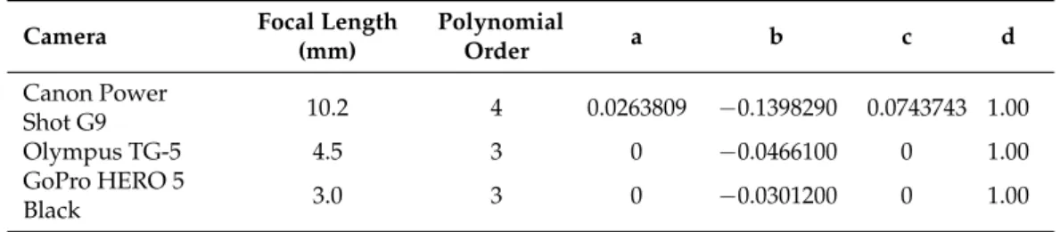
Lens distortion was corrected using a polynomial barrel inverse distortion model for the respective camera, lens, and focal length combinations with parameters obtained from the lensfun archive (https://github.com/lensfun/(Accessed on: 12 August 2020);

see Table3).

rrsc = ^r

(a∗r³+_b∗r²+_c∗r+_d) ⁽³⁾ wherer_src= target radius from central pixel,r= original image pixel,a-d= polynomial coefficients.

(7)

Table 3.Table of Distortion Parameters for Each Camera.

Camera Focal Length

(mm)

Polynomial

Order a b c d

Canon Power

Shot G9 10.2 4 0.0263809 −0.1398290 0.0743743 1.00

Olympus TG-5 4.5 3 0 −0.0466100 0 1.00

GoPro HERO 5

Black 3.0 3 0 −0.0301200 0 1.00

4. Results

4.1. Sediment Types and Distribution

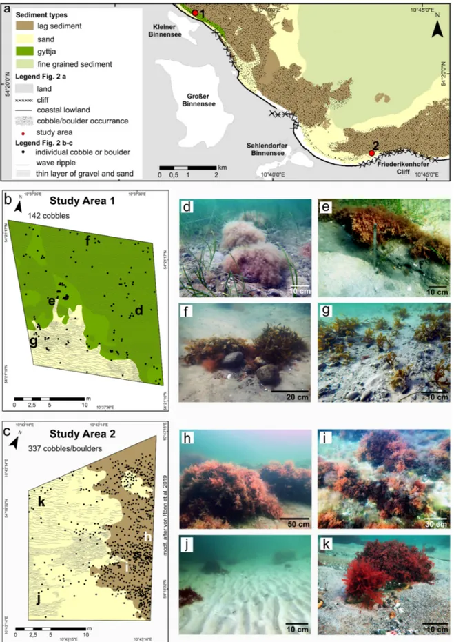
Sediments were classified into four sediment types (Figure2a)—lag sediment, sandy sediment, fine-grained sediment, and gyttja. Lag sediments were widespread and occurred particularly in front of coastal cliffs (0–20 m water depth) (Figure2a). They consisted mainly of grain sizes ranging from sand to boulders. Often, sandy sediments occurred in the shallow water zones (0–2 m water depth) parallel to the coast. Cobbles and boulders appeared occasionally within these sandy sediments. Seawards of the coastal lowland, gyttja extended alongshore and across-shore in water depths ranging from 3.5 m to 5 m.

In the area 60–100 m offshore of the gyttja, lag sediments characterized the seafloor, while fine sand occurred landwards up to the beach (Figure2a). Fine-grained sediments dominated the deepest zones (15–18 m water depth), where cobbles and boulders did not occur.

Observations by divers and sediment analyses indicated two zones within SA1, which were different in their sedimentological composition. Gyttja dominated most of the area (82%), partially covered with a thin layer of gravel and sand (Figure2b). Eelgrass grew on top of the gyttja (Figure2d,e), and cobbles were distributed on the surface as well (Figure2b,d–g). In the southern part of SA1, the gyttja formed a sharp edge with a height of 10 to 25 cm (Figure2e), followed landwards by sandy sediments (18%). Wave ripples were observed and gravel and shells occurred within the ripple troughs. Isolated cobbles or small cobble assemblages appeared within the sandy sediment (Figure2b,g). While the majority of cobbles in SA1 were colonized by macroalgae, the gravel and some small cobbles were not covered by vegetation (Figure2f,g).

SA2 is part of a seaward extending area composed of lag sediments on glacial till.

Observations by divers and sediment analyses indicated two different sedimentological zones. Unconsolidated sandy sediment characterized the southwestern part of SA2.

Within the northeastern zone, coarse sand and gravel dominated the seafloor (Figure2c).

Furthermore, a higher count of cobbles and boulders was observed, and boulders were larger. The southern zone was dominated by sandy sediments (59%) (Figure2c,j,k). Wave ripples were frequently observed within these areas, particularly in its southwestern part (Figure2c,j,k). Gravel and shells appeared in the ripple troughs. Isolated boulders or small boulder assemblages were observed within the sandy sediment (Figure2c,j,k). In contrast, mixed sediment characterized the northern zone, where grain sizes ranged from sand to gravel (41%) (Figure2c,h,i). The majority of cobbles and boulders were lying on top of the sediment, but individual boulders were not fully eroded out of the glacial till.

(8)

Figure 2. (a) Sediment distribution map of the inner Hohwacht Bay. (b) Sediment distribution and the location of all meas- ured cobbles in study area (SA)1. (d–g) Associated photographs characterizing SA1. (c) Sediment distribution of SA2 and the location of all measured cobbles and boulders. (h–k) Associated photographs of cobbles and boulders of SA2.

Figure 2. (a) Sediment distribution map of the inner Hohwacht Bay. (b) Sediment distribution and the location of all measured cobbles in study area (SA)1. (d–g) Associated photographs characterizing SA1. (c) Sediment distribution of SA2 and the location of all measured cobbles and boulders. (h–k) Associated photographs of cobbles and boulders of SA2.

(9)

4.2. Physical Habitat Structure

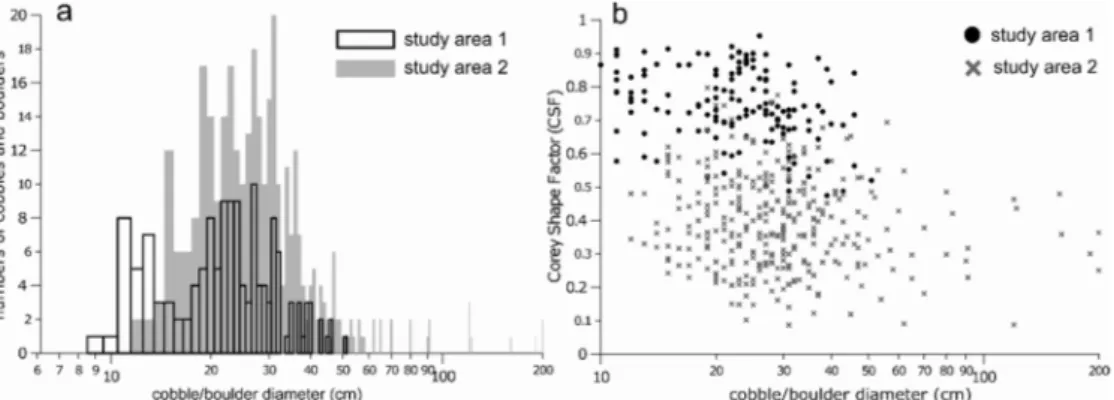
SA1: In this site, 142 cobbles were observed (Figure2b), with diameters ranging from 10 cm to 51 cm (Figure3a). On top of the gyttja, 117 cobbles were detected, while 25 cobbles were in the sandy zone. Cobbles were distributed randomly with no clear size distribution pattern. The size distribution displays high abundances of cobbles with diameters from 11 to 13 cm and from 20 to 32 cm (Figure3a). Cobbles observed in SA1 display a heterogeneous size distribution. CFS values range from 0.5 to 0.8 (Figure3b) with no correlation between size and rounding.

SA2: A total of 337 cobbles and boulders were observed (Figure2b) with diameters ranging from 12 cm to 200 cm (Figure3a). Within the lag deposits, 204 cobbles and boulders were identified and 133 within the sandy area. The size distribution displays the high abundance of diameters of 15 cm and from 19–31 cm (Figure3a), but boulder diameters from 50–200 cm were also present. High cobble and boulder accumulations occur in the northeastern zone of SA2, where boulder sizes are larger. CSF values for cobbles and boulders calculated in SA2 range from 0.1 and 0.8 (Figure3b). Boulders with diameters between 50 and 200 cm display noticeable lower CSF values (<0.6) than cobbles between 10 and 50 cm. Cobbles occurring in SA1 display a higher degree of roundness, compared to SA2 (Figure3b).

4.2. Physical Habitat Structure

SA1: In this site, 142 cobbles were observed (Figure 2b), with diameters ranging from 10 cm to 51 cm (Figure 3a). On top of the gyttja, 117 cobbles were detected, while 25 cobbles were in the sandy zone. Cobbles were distributed randomly with no clear size distribution pattern. The size distribution displays high abundances of cobbles with diameters from 11 to 13 cm and from 20 to 32 cm (Figure 3a). Cobbles observed in SA1 display a heterogeneous size distribution. CFS values range from 0.5 to 0.8 (Figure 3b) with no correlation between size and rounding.

SA2: A total of 337 cobbles and boulders were observed (Figure 2b) with diameters ranging from 12 cm to 200 cm (Figure 3a). Within the lag deposits, 204 cobbles and boulders were identified and 133 within the sandy area. The size distribution displays the high abundance of diameters of 15 cm and from 19−31 cm (Figure 3a), but boulder diameters from 50–200 cm were also present. High cobble and boulder accumulations occur in the northeastern zone of SA2, where boulder sizes are larger. CSF values for cobbles and boulders calculated in SA2 range from 0.1 and 0.8 (Figure 3b). Boulders with diameters between 50 and 200 cm display noticeable lower CSF values (<0.6) than cobbles between 10 and 50 cm. Cobbles occurring in SA1 display a higher degree of roundness, compared to SA2 (Figure 3b).

Figure 3. (a) Size distribution of all cobbles and boulders analyzed in SA1 and SA2. Sizes are di- vided into centimeter steps; note the logarithmic scale. (b) Calculated Corey shape factor (CSF) values vs. cobble/boulder sizes for SA1 and SA2 are plotted.

4.3. Benthic Community Structure

In total, 77 species were found in the sampled hard-bottom communities (Table 3).

The majority of these species belonged to the phyla Arthropoda (20), Rhodophyta (19), Cnidaria (7), and Annelida (7). The average species richness of both study areas was 30 and 31, respectively. The nMDS plot indicated differences in taxonomic community composition between the study areas (Figure S2). The samples of SA1 showed a larger spread around the group centroid than the samples of SA2. The SIMPER analysis revealed six species significantly contributing to the dissimilarity between the communities of the two study areas (Tables S1 and S2). Noticeably, these species occurred solely (Amphiblestrum auritum, Folliculina sp., Amathia gracilis, Leucosolenia botryoides, Ciona intestinalis) or mainly (Alcyonidium gelatinosum) at SA2.

4.4. Wind and Wave Conditions during Field Campaigns

The wave conditions are described by the measured (H^S) and calculated (H^{S, calc.}) significant wave heights and the maximum wave height (H^max) measured during the field campaign. To estimate wave conditions during periods in which no data are available, hindcasting was performed for the entire timeframe (Figure 4b). The hindcast of HS, calc.

generally fits the trend of the measured data. Especially, if wind directions remained stable over a longer period (1−2 days), while during short-period wind events (1−2 h) H^S are overestimated because of the assumption of a fully developed sea in the formula.

Figure 3.(a) Size distribution of all cobbles and boulders analyzed in SA1 and SA2. Sizes are divided into centimeter steps; note the logarithmic scale. (b) Calculated Corey shape factor (CSF) values vs.

cobble/boulder sizes for SA1 and SA2 are plotted.

4.3. Benthic Community Structure

In total, 77 species were found in the sampled hard-bottom communities (Table3).

The majority of these species belonged to the phyla Arthropoda (20), Rhodophyta (19), Cnidaria (7), and Annelida (7). The average species richness of both study areas was 30 and 31, respectively. The nMDS plot indicated differences in taxonomic community composition between the study areas (Figure S2). The samples of SA1 showed a larger spread around the group centroid than the samples of SA2. The SIMPER analysis revealed six species significantly contributing to the dissimilarity between the communities of the two study areas (Tables S1 and S2). Noticeably, these species occurred solely (Amphi- blestrum auritum,Folliculinasp.,Amathia gracilis,Leucosolenia botryoides,Ciona intestinalis) or mainly (Alcyonidium gelatinosum) at SA2.

4.4. Wind and Wave Conditions during Field Campaigns

The wave conditions are described by the measured (HS) and calculated (H_{S, calc.}) significant wave heights and the maximum wave height (Hmax) measured during the field campaign. To estimate wave conditions during periods in which no data are available, hindcasting was performed for the entire timeframe (Figure4b). The hindcast of H_{S, calc.}

generally fits the trend of the measured data. Especially, if wind directions remained stable over a longer period (1–2 days), while during short-period wind events (1−2 h) HSare overestimated because of the assumption of a fully developed sea in the formula.

(10)

Observation Periods

14–18 March 2018: Easterly wind directions prevailed with wind velocities of 10–14 ms⁻¹ (Figure4a). During this first period, significant wave heights ranged from HS= 0.5 m–1.3 m with Hmaxup to 2 m (Figure4b). On 16 March, H_Sdropped to 0–0.2 m, while the highest values of H_Swere registered from 15–17 March (H_S> 1.3 m). On 19 March, wind velocities decreased and the direction changed from W to N (Figure4a). 21–26 March 2018: Wind directions varied between W–SE (Figure4a), ranging in wind sectors unable to generate high energetic wave conditions due to short fetch. Significant wave heights during this period were measured at 0.3 m.

26 March–4 April 2018: Wind directions remained easterly and wind velocities varied from 5–10 ms⁻¹(Figure4a). Two peaks with H_{S, calc.}of up to 0.8 m were calculated for this period. On 29.03. values dropped to 0.1 m and rose again from 30 March to 1 April (Figure 4b). From 1–4 April, wind directions varied from W to SE, wind velocities from 2–6 ms⁻¹, and HS, calc.values remained below 0.5 m.

4–16 April 2018: During most of the time wind directions varied from W to SE and HS

values did not exceed 0.5 m (Figure4a,b). Only between 10 April and 14 April, easterly winds dominated with wind velocities varying from 5–12 ms⁻¹, and H_Svalues reached 0.9 m with corresponding Hmaxvalues of 1.5 m (Figure4a,b).

16–20 April 2018: Wind directions varied in between the sector from NW–SE and a maximum wind velocity occurred at 5 ms⁻¹. During this period, values of the HSremained below 0.4 m (Figure4b). Only on 30 April, the wind direction changed to E, and wind velocities exceeded 10 ms⁻¹, and a short peak in H_Soccurred (H_S= 0.6 m). (Figure4a).

2–7 May 2018: During the whole period, wind directions varied from SE to NW with wind velocities below 5 ms⁻¹, and H_{S, calc.}values did not exceed 0.4 m (Figure4a,b).

Observation Periods

14–18 March 2018: Easterly wind directions prevailed with wind velocities of 10–14 ms⁻¹ (Figure 4a). During this first period, significant wave heights ranged from H^S = 0.5 m–1.3 m with Hmax up to 2 m (Figure 4b). On 16 March, HS dropped to 0–0.2 m, while the highest values of HS were registered from 15–17 March (HS > 1.3 m). On 19 March, wind velocities decreased and the direction changed from W to N (Figure 4a).

21–26 March 2018: Wind directions varied between W–SE (Figure 4a), ranging in wind sectors unable to generate high energetic wave conditions due to short fetch. Signif- icant wave heights during this period were measured at 0.3 m.

26 March–4 April 2018: Wind directions remained easterly and wind velocities varied from 5−10 ms⁻¹ (Figure 4a). Two peaks with H^{S, calc.}of up to 0.8 m were calculated for this period. On 29.03. values dropped to 0.1 m and rose again from 30 March to 1 April (Figure 4b). From 1–4 April, wind directions varied from W to SE, wind velocities from 2−6 ms⁻¹, and HS, calc. values remained below 0.5 m.

4–16 April 2018: During most of the time wind directions varied from W to SE and H^S values did not exceed 0.5 m (Figure 4a,b). Only between 10 April and 14 April, easterly winds dominated with wind velocities varying from 5−12 ms⁻¹, and H^S values reached 0.9 m with corresponding Hmax values of 1.5 m (Figure 4a,b).

16–20 April 2018: Wind directions varied in between the sector from NW–SE and a maximum wind velocity occurred at 5 ms⁻¹. During this period, values of the H^S remained below 0.4 m (Figure 4b). Only on 30 April, the wind direction changed to E, and wind velocities exceeded 10 ms⁻¹, and a short peak in HS occurred (HS = 0.6m). (Figure 4a).

2–7 May 2018: During the whole period, wind directions varied from SE to NW with wind velocities below 5 ms⁻¹, and H^{S, calc.}values did not exceed 0.4 m (Figure 4a,b).

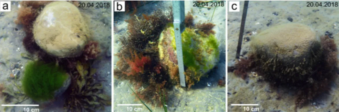
Figure 4. (a) Recalculated wind velocities and directions by inverse distance weighting (IDW) for the period 14 March–7 May 2018 using data from Kiel Lighthouse and Putlos (DWD stations). (b) Corresponding measured and calculated wave heights. (c–f) Underwater images of the same cobble (Ø 20 cm) taken at intervals (c–f) highlighted in the time series above.

(g) Average probability distribution of the number of wave events with significant wave heights (H^{S, calc.}) divided into 10 cm classes (2010−2019).

Figure 4. (a) Recalculated wind velocities and directions by inverse distance weighting (IDW) for the period 14 March–7 May 2018 using data from Kiel Lighthouse and Putlos (DWD stations). (b) Corresponding measured and calculated wave heights. (c–f) Underwater images of the same cobble (Ø 20 cm) taken at intervals (c–f) highlighted in the time series above. (g) Average probability distribution of the number of wave events with significant wave heights (H_{S, calc.}) divided into 10 cm classes (2010–2019).

(11)

4.5. Overturning of Cobbles

The overturning of most of the cobbles was observed during the field campaign (Figure 4c–f, Figure 5, and Figure S3a–d). Their overturned position is indicated by their colonized surface facing downwards, creating free space for colonization on top of the cobble (Figure5). After being overturned at least once between 14 March and 20 April, the free space on top was covered with early successional green macroalgae, which led to a mosaic of successional stages within the habitat (Figure5and Figure S3a–d).

The frequency of overturning during these periods could not be further determined.

From 14 March to 4 April and from 4–20 April, wave conditions were similar to the first period and thus must be assumed to have been strong enough to mobilize and overturn cobbles at least once (displayed cobbles Ø 20–30 cm) (Figures4c–g and5). During these periods, wind from easterly directions with velocities ranging from 10–15 ms⁻¹generated HSup to 0.8–1 m with corresponding Hmaxvalues from 1.5–2 m (Figure4a,b). Wave peak periods (TP) for measured events with HS> 0.8 m typically range from 3.6 s to 6.35 s with an average value of 5.35 s.

The probability distribution of the number of wave events with H_S≥0.8 m, from a hindcast of 10-year time series of wind, shows that these conditions occur on average 80 times per year indicating frequent overturning of cobbles in this area (Figure4g).

4.5. Overturning of Cobbles

The overturning of most of the cobbles was observed during the field campaign (Fig- ures 4c–f, 5, and S3a–d). Their overturned position is indicated by their colonized surface facing downwards, creating free space for colonization on top of the cobble (Figure 5).

After being overturned at least once between 14 March and 20 April, the free space on top was covered with early successional green macroalgae, which led to a mosaic of successional stages within the habitat (Figures 5 and S3a–d).

The frequency of overturning during these periods could not be further determined.

From 14 March to 4 April and from 4–20 April, wave conditions were similar to the first period and thus must be assumed to have been strong enough to mobilize and overturn cobbles at least once (displayed cobbles Ø 20−30 cm) (Figures 4c–g and 5). During these periods, wind from easterly directions with velocities ranging from 10–15 ms⁻¹ generated HS up to 0.8–1 m with corresponding Hmax values from 1.5–2 m (Figure 4a,b). Wave peak periods (T^P) for measured events with H^S > 0.8 m typically range from 3.6 s to 6.35 s with an average value of 5.35 s.

The probability distribution of the number of wave events with H^S ≥ 0.8 m, from a hindcast of 10-year time series of wind, shows that these conditions occur on average 80 times per year indicating frequent overturning of cobbles in this area (Figure 4g).

Figure 5. (a–c) Overturned cobbles on top of the gyttja in SA1. Free patches of space on top of the cobbles enable the growth of early successional macroalgae, leading to a mosaic of different successional stages within the habitat.

5. Discussion

The present study highlights considerable differences in the physical structure of two coastal stone habitats. The multidisciplinary approach, combining hydroacoustic data, sediment composition analyses, in situ diver measurements, benthic community analysis, and the characterization of the wave climate, provides a coherent picture of the functions and dynamics of stone habitats. The combination of spatially larger-scale hydroacoustic data and small-scale in situ measurements are important to resolve the variability of these diverse habitats in terms of three different modes of stone habitat dynamics.

5.1. Physical Habitat Structure

The majority of prior investigations on stone habitats focused on the identification and spatial extent of cobble and boulder accumulations. Other characterizations of physical habitat structures were not carried out [24,26,71]. Prior investigations focused on lag deposits and stone habitats were described as varying unsorted coarse-grained sediments ranging from gravel to boulders [14,30,61]. This is in accordance with results from SA2, where the habitat-forming cobbles and boulders are part of an area dominated by lag deposits. Here, coarse-grained sediments (sand-gravel) surround cobbles and boulders, which are characterized by a heterogeneous pattern in size (12−200 cm), in rounding degree (CSF = 0.1−0.8), and in their spatial distribution. The main source for cobbles and boulders within the southwestern Baltic Sea is the underlying glacial till and cobbles and Figure 5. (a–c) Overturned cobbles on top of the gyttja in SA1. Free patches of space on top of the cobbles enable the growth of early successional macroalgae, leading to a mosaic of different successional stages within the habitat.

5. Discussion

The present study highlights considerable differences in the physical structure of two coastal stone habitats. The multidisciplinary approach, combining hydroacoustic data, sediment composition analyses, in situ diver measurements, benthic community analysis, and the characterization of the wave climate, provides a coherent picture of the functions and dynamics of stone habitats. The combination of spatially larger-scale hydroacoustic data and small-scale in situ measurements are important to resolve the variability of these diverse habitats in terms of three different modes of stone habitat dynamics.

5.1. Physical Habitat Structure

The majority of prior investigations on stone habitats focused on the identification and spatial extent of cobble and boulder accumulations. Other characterizations of physical habitat structures were not carried out [24,26,71]. Prior investigations focused on lag deposits and stone habitats were described as varying unsorted coarse-grained sediments ranging from gravel to boulders [14,30,61]. This is in accordance with results from SA2, where the habitat-forming cobbles and boulders are part of an area dominated by lag deposits. Here, coarse-grained sediments (sand-gravel) surround cobbles and boulders, which are characterized by a heterogeneous pattern in size (12–200 cm), in rounding degree (CSF = 0.1–0.8), and in their spatial distribution. The main source for cobbles and boulders within the southwestern Baltic Sea is the underlying glacial till and cobbles and boulders

(12)

are randomly distributed within it [23,72]. Thus, a stone habitat spatially located on top of its source (glacial till) can be characterized as an autochthonous habitat since cobbles and boulders are in or near their location of the deposition.

Contrastingly, the stone habitat in SA1 is composed of a different physical structure:

Here, an overall lower—and also smaller—number of cobbles is observed (Figure2), and no boulders occur. Additionally, the cobbles show higher CSF values (0.5–0.98), compared to those observed in SA2. The discrepancy in CFS values is linked to the absence of boulders in SA1 because boulders in SA2 are clearly less rounded. Additionally, cobbles (Ø 10–50 cm) occurring in SA1 have higher CSF values, compared to cobbles of similar sizes in SA2.

Cobbles observed within SA1 are located on top of lagoonal deposits—clearly not their source material. Hence, they must have been transported on top of the lagoonal sediment and thus are described as an allochthonous habitat.

5.2. Benthic Community Structure

Differences in physical habitat structures between the study areas are reflected in the benthic communities found on cobbles and boulders as well. While no differences between SA1 and SA2 were observed in overall richness, their community structure varied.

Noticeably, those species exclusively found in SA2 were all sessile filter feeders, which are predominantly observed in the study area on larger algae such asFurcellaria lumbricalis andPhyllophora pseudoceranoïdes(personal observation). The mobility of the cobbles in SA1 might have prevented the effective establishment of these species since the succession of the communities is interrupted more frequently. The higher variability of the communities in SA1 further supports this assumption. Natural disturbances of stone habitats, which are closely linked to the mobility of the substrate, have been shown as an important determinant of the benthic communities in previous studies [73]. Especially filter-feeding organisms are known to be sensitive against sedimentation effects since their feeding apparatus can be clogged [74,75]. Therefore, it appears likely that these disturbance-related effects were responsible for the observed differences in community structure [76].

5.3. Exposure of New Cobbles and Boulders

Within both study areas, the majority of cobbles and boulders are scattered on top of the surrounding sediments. They are characterized as potentially unstable [24,39]. In SA2, single boulders are observed, which are not fully eroded out of the glacial till—they are classified as stable. We assume a further exposure of these boulders and subsequent addition of cobbles and boulders to the habitat by ongoing erosion of the glacial till [22].

A spatial extension of the stone habitat is not expected, but rather a continuous growth of the habitat structure providing more space for organisms to settle (Figure6). Investigations carried out at the nearby Stohler Kliff und Boknis Eck (Kiel Bight) support this assumption as an increase of boulders over several decades was observed [22]. The degree and rate of this hereby, depend on respective abrasion rates [22,25,30], which range from 1–5 cm/year (up to a water depth of 7 m), depending on water depth, wave climate, and resistance of the glacial till against erosion [77].

5.4. Overturning of Cobbles

Changes within the physical habitat structure connected to timescales of seconds or minutes occur as cobbles are overturned by wave action. The frequent overturning of small- and medium-sized cobbles (up to 12 cm) has been investigated in intertidal areas [36,78] and in shallow subtidal zones (2–5 m water depth) [37,38]. Within SA1, we observed the overturning of a medium-sized cobble (Ø 20 cm, 3.5 m water depth) twice, during two different storm events when significant wave heights up to 1.3 m with Hmaxranging from 1.5 m to 2 m persisted over several days. Recalculations of wave heights for SA1 for the last 10 years reveal a regular occurrence of these conditions in SA1 (HS≥0.8 m) for about 80 events/year (Figure4g). Further cobbles were observed to have been overturned with their colonized side facing down or presenting a “monks

(13)

head” pattern (Figure5and Figure S3), which indicate regular overturning as well [36,79].

Therefore, it is assumed that cobbles within SA1 are overturned several times per year (Figure6).

Overturning of cobbles exposes empty settling space for benthic organisms [36,37].

The overturning depends on the size of the cobble, water depth, and wave climate; hence, recolonization of the empty spaces leads to a variety of successional stages within a habitat [36,38,79]. This is in accordance with the results from SA1, where the growth of early successional macroalgae was observed after the overturning of cobbles. Furthermore, different successional stages were observed on a cobble, which was only rotated by about 90^◦. The existing macroalgae survived and additionally early successional macroalgae developed on the free patch (Figure5a,b). Similar results have been described for intertidal zones, where the “successional age” of a cobble did not return to zero after overturning since some algae survived and regrew vegetatively [36].

m) for about 80 events/year (Figure 4g). Further cobbles were observed to have been overturned with their colonized side facing down or presenting a “monks head” pattern (Fig- ures 5 and S3), which indicate regular overturning as well [36,79]. Therefore, it is assumed that cobbles within SA1 are overturned several times per year (Figure 6).

Overturning of cobbles exposes empty settling space for benthic organisms [36,37].

The overturning depends on the size of the cobble, water depth, and wave climate; hence, recolonization of the empty spaces leads to a variety of successional stages within a habitat [36,38,79]. This is in accordance with the results from SA1, where the growth of early successional macroalgae was observed after the overturning of cobbles. Furthermore, different successional stages were observed on a cobble, which was only rotated by about 90°.

The existing macroalgae survived and additionally early successional macroalgae developed on the free patch (Figure 5a,b). Similar results have been described for intertidal zones, where the “successional age” of a cobble did not return to zero after overturning since some algae survived and regrew vegetatively [36].

Figure 6. Conceptual model of the dynamics of stone habitats. 1. Exposure of “new” cobbles and boulders from the glacial till by abrasion. 2. Overturning of cobbles and boulders creating empty hard ground for organisms to settle. 3. Migration of cobbles and boulders out of the autochthonous habitat (lag sediments), creating a new allochthonous habitat or expanding the existing habitat.

5.5. Migration of Cobbles

Coastal stone habitats are not only dynamic as their physical habitat structure changes on disparate timescales (exposure and overturning), but also on longer timescales. Cobbles in SA1 are located on gyttja. This sediment facies, which developed during the Holocene on top of the glacial till, can only develop during explicitly low-energy conditions [46,47]. During those conditions, cobbles and boulders cannot be mobilized. Since cobbles are now observed on top of the gyttja (up to Ø 50 cm), they must have been transported from their initial location during higher-energy conditions after the development of the gyttja (Figure 6). Larger cobbles and boulders (>10 cm) within the southwestern Baltic Sea have been considered to be comparatively stable by some authors [27–29], Figure 6.Conceptual model of the dynamics of stone habitats.1.Exposure of “new” cobbles and boulders from the glacial till by abrasion.2.Overturning of cobbles and boulders creating empty hard ground for organisms to settle.3.Migration of cobbles and boulders out of the autochthonous habitat (lag sediments), creating a new allochthonous habitat or expanding the existing habitat.

5.5. Migration of Cobbles

Coastal stone habitats are not only dynamic as their physical habitat structure changes on disparate timescales (exposure and overturning), but also on longer timescales. Cobbles in SA1 are located on gyttja. This sediment facies, which developed during the Holocene on top of the glacial till, can only develop during explicitly low-energy conditions [46,47].

During those conditions, cobbles and boulders cannot be mobilized. Since cobbles are now observed on top of the gyttja (up to Ø 50 cm), they must have been transported from their initial location during higher-energy conditions after the development of the gyttja (Figure6). Larger cobbles and boulders (>10 cm) within the southwestern Baltic Sea have been considered to be comparatively stable by some authors [27–29], whereas others, similar to our observations, indicated the frequent mobility of gravel and small cobbles by wave action in up to 5.6 m water depth [30].

(14)

As described previously, cobbles within SA1 show higher degrees of roundness, compared to those in SA2. Generally, the transport of cobbles leads to increased roundness [58,80]. In this case, we do not expect that cobbles are more rounded by the transport into SA1 since the distance to the next seaward lying lag deposit is rather short (60–100 m).

We assume that they were transported because of their already high degree of roundness since, along with the pretransport environment, the shape and size influence the transport distance [81,82]. Schrottke et al. (2006) show the mobility of small cobbles originating from lag deposits in water depth from 3.4 m up to 5.6 m with a mainly landward transport direction [30]. Thus, we expect that cobbles in SA1 originated from the seaward lag sediment deposits (Figure6). The type of transport was not further investigated, but the sliding, rolling, and saltation may be enhanced by algae-assisted transport (lift and drag). This has been described often as a wave-driven, landward transport agent of gravel or cobbles with attached macroalgae, reducing the critical stress required for transport by as much as 92% [83–85].

6. Conclusions

Coastal stone habitats vary in their physical habitat characteristics, dynamics, and benthic community composition. In the past, these habitats generally have been described as varying unsorted coarse-grained sediments ranging from gravel to boulders within lag deposits, commonly considered rather stable environments.

Based on the data from Hohwacht Bay, we discuss the dynamics of stone habitats as follows: Three modes of wave-induced processes change the physical structure and colonization potential. Exposure of cobbles and boulders from glacial till by erosion of the fine matrix is the main source and happens on timescales of decades. Overturning of cobbles by wave action happens instantaneously at supercritical wave conditions and is connected to frequent recolonization. Migration of cobbles happens locally and into areas far from the source region of glacial till deposits. It should be understood that the modes do not only occur separately but also act simultaneously, characterizing stone habitats as very dynamic on different timescales.

Two classes may be distinguished: On the one hand, autochthonous stone habitats, which are bound to their source region, and on the other hand, allochthonous stone habitats, which develop by accumulation of migrated cobbles, extending or forming habitats at areas far from the source region.

These results highlight natural dynamic processes of coastal stone habitats, which should be considered in marine habitat mapping directives and in projects of ecological engineering or restoration of these habitats.

Supplementary Materials:The following are available online athttps://www.mdpi.com/article/

10.3390/geosciences11040171/s1, Figure S1a–c: SSS Mosaic of the inner Hohwacht Bay, Figure S2:

nMDS plot based on Bray–Curtis dissimilarities, Figure S3a–d: Cobbles observed during field campaign, Table S1: Species identified from the sampled hard-bottom communities. Table S2:

Similarity percentage (SIMPER) analysis comparing the two study areas.

Author Contributions: Conceptualization, G.A.v.R. and C.W.; methodology, G.A.v.R. and K.S.;

formal analysis, G.A.v.R., K.K., and M.F.; investigation, G.A.v.R. and M.F.; writing—original draft preparation, G.A.v.R.; writing—review and editing, G.A.v.R., C.W., K.S., K.K., M.F., and H.-C.R.;

visualization, G.A.v.R., K.S., and C.W.; supervision, C.W. and K.S.; project administration, K.S.

All authors have read and agreed to the published version of the manuscript.

Funding: This research resulted from the project Geo-Habitats Baltic Sea Germany Schleswig- Holstein (GeoHab BALDESH), a research and development cooperation between the Kiel University and the State Agency for Agriculture, Environment and Rural Areas—Schleswig-Holstein (LLUR).

The project is financed by the State Agency for Agriculture, Environment and Rural Areas—Schleswig- Holstein (LLUR). We acknowledge financial support by Land Schleswig-Holstein within the funding program Open Access Publikationsfonds.

(15)

Acknowledgments: We would like to thank Eric Steen for the configuration of the survey equip- ment and Nils Steinfeld for his support during our research surveys. We thank Daniel Unverricht, Pushpa Dissanayake, and Marius Becker for their constructive discussions. We also thank Christoph Heinrich for his support and good ideas. We thank the two anonymous reviewers for their helpful and constructive comments, which improved the manuscript. We would like to thank the research divers of Kiel University for their valuable fieldwork and Renate Schütt and Gesche Bock for their pa- tient support during species identification. We also wish to thank the captain and crew of the research vessel Littorina for their excellent support at all times.

Conflicts of Interest:The authors declare no conflict of interest.

References

1. Liversage, K. The influence of boulder shape on the spatial distribution of crustose coralline algae (Corallinales, Rhodophyta).

Mar. Ecol.2016,37, 459–462. [CrossRef]

2. Lefcheck, J.S.; Hughes, B.B.; Johnson, A.J.; Pfirrmann, B.W.; Rasher, D.B.; Smyth, A.R.; Williams, B.L.; Beck, M.W.; Orth, R.J.

Are coastal habitats important nurseries? A meta-analysis.Conserv. Lett.2019,12, e12645. [CrossRef]

3. Gallucci, F.; Christofoletti, A.R.; Fonseca, G.; Dias, M.G. The effects of habitat heterogeneity at distinct spatial scales on hard- bottom-associated communities.Diversity2020,12, 39. [CrossRef]

4. Kolp, O. Die sedimente der westlichen und südlichen ostsee und ihre darstellung.Beiträge Meereskd.1966,17–18, 9–60.

5. Sebens, K.P. Habitat structure and community dynamics in marine benthic systems. InHabitat Structure: The Physical Arrange- ment of Objects in Space; Bell, S.S., McCoy, E.D., Mushinsky, H.R., Eds.; Population and Community Biology Series; Springer:

Dordrecht, The Netherlands, 1991; pp. 211–234. ISBN 978-94-011-3076-9.

6. Archambault, P.; Bourget, E. Scales of coastal heterogeneity and benthic intertidal species richness, diversity and abundance.

Mar. Ecol. Prog. Ser.1996,136, 111–121. [CrossRef]

7. Kovalenko, K.E.; Thomaz, S.M.; Warfe, D.M. Habitat complexity: Approaches and future directions.Hydrobiologia2012,685, 1–17.

[CrossRef]

8. Mikkelsen, L.; Mouritsen, K.; Dahl, J.; Teilmann, J.; Tougaard, J. Re-established stony reef attracts harbour porpoises phocoena phocoena.Mar. Ecol. Prog. Ser.2013, 238–248. [CrossRef]

9. Kristensen, L.D.; Støttrup, J.G.; Svendsen, J.C.; Stenberg, C.; Hansen, O.K.H.; Grønkjær, P. Behavioural changes of atlantic cod (gadus morhua) after marine boulder reef restoration: Implications for coastal habitat management and natura 2000 areas.

Fish. Manag. Ecol.2017,24, 353–360. [CrossRef]

10. Torn, K.; Herkül, K.; Martin, G.; Oganjan, K. Assessment of quality of three marine benthic habitat types in Northern Baltic Sea.

Ecol. Indic.2017,73, 772–783. [CrossRef]

11. Rönnbäck, P.; Kautsky, N.; Pihl, L.; Troell, M.; Söderqvist, T.; Wennhage, H. Ecosystem goods and services from swedish coastal habitats: Identification, valuation, and implications of ecosystem shifts.Ambio2007,36, 534–544. [CrossRef]

12. Snoeijs-Leijonmalm, P.; Schubert, H.; Radziejewska, T.Biological Oceanography of the Baltic Sea; Springer Science & Business Media:

Dordrecht, The Netherlands, 2017; ISBN 978-94-007-0668-2. [CrossRef]

13. Lappalainen, J.; Virtanen, E.A.; Kallio, K.; Junttila, S.; Viitasalo, M. Substrate limitation of a habitat-forming genus fucus under different water clarity scenarios in the Northern Baltic Sea.Estuar. Coast. Shelf Sci.2019,218, 31–38. [CrossRef]

14. Papenmeier, S.; Darr, A.; Feldens, P.; Michaelis, R. Hydroacoustic mapping of geogenic hard substrates: Challenges and review of german approaches.Geosciences2020,10, 100. [CrossRef]

15. The European Parliament; The Council Of The European Union. Directive 2008/56/EC of the European Parliament and of the Council of 17 June 2008 Establishing a Framework for Community Action in the Field of Marine Environmental Policy (Marine Strategy Framework Directive). 2008. Available online:https://eur-lex.europa.eu/legal-content/EN/TXT/PDF/?uri=CELEX:

32008L0056&from=en(accessed on 7 April 2021).

16. The Council Of The European Communities. Directive 92/43/EEC on the Conservation of Natural Habitats and of Wild Fauna and Flora (Habitat Directive). 1992. Available online:http://extwprlegs1.fao.org/docs/pdf/eur34772.pdf(accessed on 7 April 2021).

17. Winter, C. Monitoring concepts for an evaluation of marine environmental states in the german bight. Geo. Mar. Lett2017, 37, 75–78. [CrossRef]

18. Brown, E.J.; Vasconcelos, R.P.; Wennhage, H.; Bergström, U.; Støttrup, J.G.; van de Wolfshaar, K.; Millisenda, G.; Colloca, F.;

Le Pape, O. Conflicts in the coastal zone: Human impacts on commercially important fish species utilizing coastal habitat.ICES J.

Mar. Sci.2018,75, 1203–1213. [CrossRef]

19. Bertocci, I.; Dell’Anno, A.; Musco, L.; Gambi, C.; Saggiomo, V.; Cannavacciuolo, M.; Martire, M.L.; Passarelli, A.; Zazo, G.;

Danovaro, R. Multiple human pressures in coastal habitats: Variation of meiofaunal assemblages associated with sewage discharge in a post-industrial area.Sci. Total Environ.2019,655, 1218–1231. [CrossRef]

20. Bock, G.; Thiermann, F.; Rumohr, H.; Karez, R. Ausmaß der Steinfischerei an der schleswig-holsteinischen Ostseeküste.Jahres- ber. Landesamt Natur Umwelt Landes Schleswig-Holst.2003,8, 111–116.