2 f CO :amesocosmstudyintheeasternBalticSea Alterationsinmicrobialcommunitycompositionwithincreasing

(1)

https://doi.org/10.5194/bg-14-3831-2017

Alterations in microbial community composition with increasing f CO ₂ : a mesocosm study in the eastern Baltic Sea

Katharine J. Crawfurd¹, Santiago Alvarez-Fernandez², Kristina D. A. Mojica³, Ulf Riebesell⁴, and Corina P. D. Brussaard^1,5

1NIOZ Royal Netherlands Institute for Sea Research, Department of Marine Microbiology and Biogeochemistry and Utrecht University, PO Box 59, 1790 AB Den Burg, Texel, the Netherlands

2Alfred-Wegener-Institut Helmholtz-Zentrum für Polar- und Meeresforschung, Biologische Anstalt Helgoland, 27498 Helgoland, Germany

3Department of Botany and Plant Pathology, Cordley Hall 2082, Oregon State University, Corvallis, Oregon 97331-29052, USA

4GEOMAR Helmholtz Centre for Ocean Research Kiel, Biological Oceanography, Düsternbrooker Weg 20, 24105 Kiel, Germany

5Aquatic Microbiology, Institute for Biodiversity and Ecosystem Dynamics, University of Amsterdam, PO Box 94248, 1090 GE Amsterdam, the Netherlands

Correspondence to:Katharine J. Crawfurd (kate.crawfurd@gmail.com) and Corina P. D. Brussaard (corina.brussaard@nioz.nl)

Received: 28 November 2015 – Discussion started: 2 February 2016

Revised: 24 June 2017 – Accepted: 3 July 2017 – Published: 29 August 2017

Abstract. Ocean acidification resulting from the uptake of anthropogenic carbon dioxide (CO2) by the ocean is considered a major threat to marine ecosystems. Here we ex- amined the effects of ocean acidification on microbial community dynamics in the eastern Baltic Sea during the summer of 2012 when inorganic nitrogen and phosphorus were strongly depleted. Large-volume in situ mesocosms were employed to mimic present, future and far future CO₂ sce- narios. All six groups of phytoplankton enumerated by flow cytometry (<20 µm cell diameter) showed distinct trends in net growth and abundance with CO₂ enrichment. The picoeukaryotic phytoplankton groups Pico-I and Pico-II displayed enhanced abundances, whilst Pico-III, Synechococ- cusand the nanoeukaryotic phytoplankton groups were negatively affected by elevated fugacity of CO2(fCO2). Specif- ically, the numerically dominant eukaryote, Pico-I, demon- strated increases in gross growth rate with increasingfCO2

sufficient to double its abundance. The dynamics of the prokaryote community closely followed trends in total algal biomass despite differential effects offCO₂on algal groups.

Similarly, viral abundances corresponded to prokaryotic host population dynamics. Viral lysis and grazing were both im-

portant in controlling microbial abundances. Overall our results point to a shift, with increasingfCO2, towards a more regenerative system with production dominated by small picoeukaryotic phytoplankton.

1 Introduction

Marine phytoplankton are responsible for approximately half of global primary production (Field et al., 1998) with shelf sea communities contributing an average of 15–30 % (Kuli´nski and Pempkowiak, 2011). Since the industrial rev- olution, atmospheric carbon dioxide (CO2) concentrations have increased by nearly 40 % due to anthropogenic emis- sions, primarily caused by the burning of fossil fuels and deforestation (Doney et al., 2009). Atmospheric CO₂ dis- solves in the oceans where it forms carbonic acid that re- duces seawater pH, which is a process commonly termed ocean acidification (OA). Currently, along with warming sea surface temperatures and changing light and nutrient conditions, marine ecosystems face unprecedented decreases in ocean pH (Doney et al., 2009; Gruber, 2011). Ocean acid-

(2)

ification is considered one of the greatest current threats to marine ecosystems (Turley and Boot, 2010) and has been shown to alter phytoplankton primary production with the direction and magnitude of the responses dependent on community composition (e.g. Hein and Sand-Jensen, 1997;

Tortell et al., 2002; Leonardos and Geider, 2005; Engel et al., 2008; Feng et al., 2009; Eberlein et al., 2017). Cer- tain cyanobacteria, including diazotrophs, demonstrate stimulated growth under conditions of elevated CO₂ (Qiu and Gao, 2002; Barcelos e Ramos et al., 2007; Hutchins, et al., 2007; Dutkiewicz et al., 2015). However, no consistent trends have been found for Synechococcus (Schulz et al., 2017 and references therein). The responses of diatoms and coccolithophores also appear more variable (Dutkiewicz et al., 2015 and references therein), although coccolithophore calcification seems generally negatively impacted (Meyer and Riebesell, 2015; Riebesell et al., 2017). OA has also been reported to increase the abundances of small-sized photoautotrophic eukaryotes in mesocosm experiments (Engel et al., 2008; Meakin and Wyman, 2011; Brussaard et al., 2013;

Schulz et al., 2017).

Recently, data regarding the effects of OA on taxa-specific phytoplankton growth rates were incorporated into a global ecosystem model. The results emphasized that elevated CO₂ concentrations can cause changes in community structure by altering the competitive fitness and thus the competition between phytoplankton groups (Dutkiewicz et al., 2015). More- over, OA was found to have a greater impact on phytoplankton community size structure, function and biomass than either warming or reduced nutrient supply (Dutkiewicz et al., 2015). Many OA studies have been conducted using single species under controlled laboratory conditions and therefore cannot account for intrinsic community interactions that occur under natural conditions. Alternatively, larger-volume mesocosm experiments allow for OA manipulation of natural communities, and are more likely to capture and quantify the overall response of the natural ecosystems. To date, the majority of these experiments started under replete nutrient conditions or received nutrient additions (Paul et al., 2015 and references therein). Thus, limited data are available for oligotrophic conditions, which are present in ∼75% of the world’s oceans (Corno et al., 2007).

Whilst environmental factors, such as temperature, light, nutrient and CO2concentrations, regulate gross primary production, loss factors determine the fate of this photosynthetically fixed carbon. Grazing, sinking and viral lysis affect the cycling of elements in different manners, i.e. transferred to higher trophic levels through grazing, carbon sequestra- tion in deep waters and sediments, and cellular content re- lease by viral lysis (Wilhelm and Suttle, 1999; Brussaard et al., 2005). Released detrital and dissolved organic matter (DOM) is quickly utilized by heterotrophic bacteria, thereby stimulating activity within the microbial loop (Brussaard et al., 2008; Lønborg et al., 2013; Sheik et al., 2014; Middelboe and Lyck, 2002). Consequently, bacteria may be affected in-

directly by OA through changes in the quality and/or quan- tity of DOM (Weinbauer et al., 2011). Viral lysis has been found to be as important as microzooplankton grazing to the mortality of natural bacterioplankton and phytoplankton (Weinbauer, 2004; Baudoux et al., 2006; Evans and Brus- saard, 2012; Mojica et al., 2016). Thus far, most studies ex- amining the effects of OA on microzooplankton abundance and/or grazing have found little or no direct effect (Suffrian et al., 2008; Rose et al., 2009; Aberle et al., 2013; Brussaard et al., 2013; Niehoff et al., 2013). To our knowledge, no viral lysis rates have been reported for natural phytoplankton communities under conditions of OA. A few studies have inferred rates based on changes in viral abundances under enhanced CO2, but the results are inconsistent (Larsen et al., 2008;

Brussaard et al., 2013). Therefore, the effect of OA on the relative share of these key loss processes is still understudied for most ecosystems.

Here we report on the temporal dynamics of microbes (phytoplankton, prokaryotes and viruses) under the influence of enhanced CO₂concentrations in the low-salinity (around 5.7) Baltic Sea. Using large mesocosms with in situ light and temperature conditions, the pelagic ecosystem was ex- posed to a range of increasing CO₂concentrations from am- bient to future and far future concentrations. The study was performed during the summer in the Baltic Sea near Tvär- minne when conditions were oligotrophic. Our data show that over the 43-day experiment, enhanced CO2 concentrations elicited distinct shifts in the microbial community, most notably an increase in the net growth of small picoeukaryotic phytoplankton.

2 Materials and methods

2.1 Study site and experimental set-up

The present study was conducted in the Tvärminne Storfjär- den (59^◦51.5⁰N, 23^◦15.5⁰E) between 14 June and 7 August 2012. Nine mesocosms, each enclosing∼55 m³ of water, were moored in a square arrangement at a site with a water depth of approximately 30 m. The mesocosms consisted of open-ended polyurethane bags 2 m in diameter and 18.5 m in length mounted onto floating frames covered at each end with a 3 mm mesh. Initially, the mesocosms were kept open for 5 days to allow for rinsing and water exchange while ex- cluding large organisms from entering with the 3 mm mesh.

During this time, the bags were positioned such that the tops were submerged 0.5 m below the water surface and the bot- toms reached down to 17 m of depth in the water column.

Photosynthetically active radiation (PAR) transparent plastic hoods (open on the side) prevented rain and bird droppings from entering the mesocosms, which would affect salinity and nutrients, respectively. Five days before the CO₂ treatment was to begin, the water column of the mesocosms was isolated from the influence of the surrounding water. To do

(3)

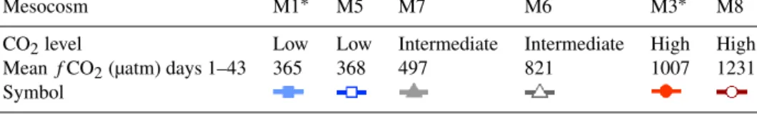
Table 1.ThefCO₂concentrations (µatm) averaged over the duration of the experiment (following CO₂addition) and subsequent classifi- cation as low, intermediate or high. Mesocosms sampled for mortality assays are denoted by an asterisk. The symbols and colours are used throughout this paper and the corresponding articles in this issue.

Mesocosm M1^∗ M5 M7 M6 M3^∗ M8

CO₂level Low Low Intermediate Intermediate High High

MeanfCO₂(µatm) days 1–43 365 368 497 821 1007 1231

Symbol

so, the 3 mm mesh was removed and sediment traps (2 m long) were attached to close off the bottom of the mesocosms. The top ends of the bags were raised and secured to the frame 1.5 m above the water surface to prevent water from entering via wave action. The mesocosms were then bubbled with compressed air for 3.5 min to remove salinity gradients and ensure that the water body was fully homoge- neous.

The present paper includes results from only six of the original mesocosms due to the unfortunate loss of three mesocosms, which were compromised by leakage. The mean fugacity of CO₂ (fCO₂) during the experiment, i.e. days 1–43, for the individual mesocosms were as follows: M1, 365 µatm; M3, 1007 µatm; M5, 368 µatm; M6, 821 µatm; M7, 497 µatm; M8, 1231 µatm (Table 1). The gradient of non- replicatedfCO₂in the present study (as opposed to a smaller number of replicated treatment levels) was selected as a bal- ance between the necessary but manageable number of mesocosms and to minimize the impact of the high loss potential for the mesocosms to successfully address the under- lying questions of the study (Schulz and Riebesell, 2013).

Moreover, it maximizes the potential of identifying a threshold fCO2 level concentration if present (by allowing for a larger number of treatment levels). Carbon dioxide manipulation was carried out in four steps and took place between days 0 and 4 until the target fCO₂ was reached. The initial fCO₂ was 240 µatm. ForfCO₂ manipulations, 50 µm filtered natural seawater was saturated with CO₂ and then injected evenly throughout the depth of the mesocosms as described by Riebesell et al. (2013). Two mesocosms func- tioned as controls and were treated in a similar manner using only filtered seawater. On day 15, a supplementary fCO₂ addition was made to the top 7 m of mesocosms numbered 3, 6 and 8 to replace CO2 lost due to outgassing (Paul et al., 2015; Spilling et al., 2016). Throughout this study we refer to fCO2, which accounts for the nonideal behaviour of CO2gas and is considered the standard measurement re- quired for gas exchange (Pfeil et al., 2013).

Initial nutrient concentrations were 0.05, 0.15, 6.2 and 0.2 µmol L⁻¹for nitrate, phosphate, silicate and ammonium, respectively. Nutrient concentrations remained low for the duration of the experiment (Paul et al., 2015; this issue) and no nutrients were added. Salinity was relatively con- stant around 5.7. Temperature was more variable; on aver-

age temperature within the mesocosms (0–17 m) increased from∼8^◦C to a maximum on day 15 of∼15^◦C and then decreased again to∼8^◦C by day 30. For further details of the experimental set-up, carbonate chemistry dynamics and nutrient concentrations throughout the experiment we refer to the general overview paper by Paul et al. (2015).

Collective sampling was performed every morning using depth-integrated water samplers (IWS; Hydro-Bios, Kiel).

These sampling devices were gently lowered through the water column collecting ∼5 L of water gradually between 0 and 10 m (top) or 0 and 17 m (whole water column). Water was collected from all mesocosms and the surrounding water. Subsamples were obtained for the enumeration of phytoplankton, prokaryotes and viruses. Samples for viral lysis and grazing experiments were taken from 5 m of depth using a gentle vacuum-driven pump system. Samples were protected against sunlight and warming by thick black plastic bags containing wet ice. Samples were processed at in situ temperature (representative of 5 m of depth) under dim light and han- dled using nitrile gloves. As viral lysis and grazing rates were determined from samples taken from 5 m of depth, the samples for microbial abundances reported here were taken from the top 10 m integrated samples.

The experimental period has been divided into four phases based on major physical and biological changes (Paul et al., 2015): Phase 0 before CO₂ addition (days −5 to 0), Phase I (days 1–16), Phase II (days 17–30) and Phase III (days 31–43). Throughout this paper, the data are presented using three colours (blue, grey and red), representing low (mesocosms M1 and M5), intermediate (M6 and M7) and high (M3 and M8)fCO₂levels (Table 1).

2.2 Microbial abundances

Microbes were enumerated using a Becton Dickinson FAC- SCalibur flow cytometer (FCM) equipped with a 488 nm ar- gon laser. The samples were stored on wet ice and in the dark until counting. The photoautotrophic cells (<20 µm) were counted directly using fresh seawater and were discriminated by their autofluorescent pigments (Marie et al., 1999).

Six phytoplankton clusters were differentiated based on the bivariant plots of either chlorophyll (red autofluorescence) or phycoerythrin (orange autofluorescence forSynechococ- cus and Pico-III) against side scatter. The size of the different phytoplankton clusters was determined by gentle fil-

(4)

tration through 25 mm diameter polycarbonate filters (What- man) with a range of pore sizes (12, 10, 8, 5, 3, 2, 1 and 0.8 µm) according to Veldhuis and Kraay (2004). Average cell sizes for the different phytoplankton groups were 1, 1, 3, 2.9, 5.2 and 8.8 µm in diameter for the prokaryotic cyanobac- teriaSynechococcusspp. (SYN), picoeukaryotic phytoplankton I, II and III (Pico-I–III) and nanoeukaryotic phytoplankton I and II (Nano-I, Nano-II), respectively. Pico-III was discriminated from Pico-II (comparable average cell size) by a higher orange autofluorescence signature, potentially representing small-sized cryptophytes (Klaveness, 1989) or, alternatively, large single cells or microcolonies of Synechococ- cus (Haverkamp et al., 2009). The cyanobacterial species Prochlorococcusspp. were not observed during this experiment. Counts were converted to cellular carbon by assuming a spherical shape equivalent to the average cell diameters determined from size fractionations and applying conversion factors of 237 fg C µm⁻³ (Worden et al., 2004) and 196.5 fg C µm⁻³(Garrison et al., 2000) for pico- and nano- sized plankton, respectively. Microbial net growth and loss rates were derived from exponential regressions of changes in the cell abundances over time.

Abundances of prokaryotes and viruses were determined from 0.5 % glutaraldehyde fixed, flash-frozen (−80^◦C) samples according to Marie et al. (1999) and Brussaard (2004).

The prokaryotes include heterotrophic bacteria, archaea and unicellular cyanobacteria, the latter accounting for a maxi- mal 10 % of the total abundance in our samples as indicated by their autofluorescence. Thawed samples were diluted with sterile autoclaved Tris-EDTA buffer (10 mM Tris-HCl and 1 mM EDTA; pH 8.2; Mojica et al., 2014) and stained with the green fluorescent nucleic acid-specific dye SYBR Green I (Invitrogen Inc.) to a final concentration of the commer- cial stock of 1.0×10⁻⁴(for prokaryotes) or 0.5×10⁻⁴(for viruses). Virus samples were stained at 80^◦C for 10 min and then allowed to cool for 5 min at room temperature in the dark. Prokaryotes were stained for 15 min at room temperature in the dark (Brussaard, 2004). Prokaryotes and viruses were discriminated in bivariate scatter plots of green fluorescence versus side scatter. Final counts were corrected for blanks prepared and analysed in a similar manner as the samples. Two groups of prokaryotes were identified by their stained nucleic acid fluorescence, referred here on as low (LNA) and high (HNA) fluorescence prokaryotes.

2.3 Viral lysis and grazing

Microzooplankton grazing and viral lysis of phytoplankton was determined using the modified dilution assay based on reducing grazing and viral lysis mortality pressure in a serial manner allowing for increased phytoplankton growth (over the incubation period) with dilution (Mojica et al., 2016).

Two dilution series were created in clear 1.2 L polycarbonate bottles by gently mixing 200 µm sieved whole seawater with either 0.45 µm filtered seawater (i.e. microzooplankton

grazers removed) or 30 kDa filtered seawater (i.e. grazers and viruses removed) to final dilutions of 20, 40, 70 and 100 %.

The 0.45 µm filtrate was produced by gravity filtration of 200 µm mesh sieved seawater through a 0.45 µm Sartopore capsule filter. The 30 kDa ultrafiltrate was produced by tangential flow filtration of 200 µm pre-sieved seawater using a 30 kDa Vivaflow 200 PES membrane tangential flow car- tridge (Vivascience). All treatments were performed in triplicate. Bottles were suspended next to the mesocosms in small cages at 5 m of depth for 24 h. Subsamples were taken at 0 and 24 h, and phytoplankton abundances of the grazing series (0.45 µm diluent) were enumerated by flow cytometry. Due to time constraints, the majority of the samples of the 30 kDa series were fixed with 1 % (final concentration) formalde- hyde : hexamine solution (18 %v/v: 10 %w/v) for 30 min at 4^◦C, flash-frozen in liquid nitrogen and stored at−80^◦C until flow cytometry analysis in the home laboratory. Fixation had no significant effect (Student’sttests;pvalue>0.05) as tested periodically against fresh samples. The modified dilution assay was only run for mesocosms 1 (lowfCO₂) and 3 (highfCO₂) due to the logistics of handling times. Exper- iments were performed until day 31. Grazing rates and the combined rate of grazing and viral lysis were estimated from the slope of a regression of phytoplankton apparent growth versus dilution of the 0.45 µm and 30 kDa series, respectively. A significant difference between the two regression coefficients (as tested by analysis of covariance) indicated a significant viral lysis rate. Phytoplankton gross growth rate, in the absence of grazing and viral lysis, was derived from the y-intercept of the 30 kDa series regression. Similarly, significant differences between mesocosms M1 and M3 (low and highfCO₂) were determined through an analysis of covariance of the dilution series for the two mesocosms. A significance threshold of 0.05 was used, and significance is denoted throughout the paper by an asterisk (^∗). Occasionally, the regression of apparent growth rate versus fraction of natural water resulted in a positive slope (thus no reduction in mortality with dilution). In addition, very low phytoplankton abundances can also prohibit the statistical significance of results. Under such conditions dilution experiments were deemed unsuccessful (for limitations of the modified dilution method, see Baudoux et al., 2006; Kimmance and Brussaard, 2010; Stoecker et al., 2015).

Viral lysis of prokaryotes was determined according to the viral production assay (Wilhelm et al., 2002; Winget et al., 2005). After reduction of the natural virus concentration, new virus production by the natural bacterial community is sampled and tracked over time (24 h). Free viruses were reduced from a 300 mL sample of whole water by re- circulation over a 0.2 µm pore size polyether sulfone membrane (PES) tangential flow filter (Vivaflow 50; Vivascience) at a filtrate expulsion rate of 40 mL min⁻¹. The concentrated sample was then reconstituted to the original volume using virus-free seawater. This process was repeated a total of three times to gradually wash away viruses. After the final recon-

(5)

stitution, 50 mL aliquots were distributed into six polycarbonate tubes. Mitomycin C (Sigma-Aldrich; final concentration 1 µg mL⁻¹; maintained at 4^◦C), which induces lyso- genic bacteria (Weinbauer and Suttle, 1996) was added to a second series of triplicate samples for each mesocosm. A third series of incubations with 0.2 µm filtered samples was used as a control for viral loss (e.g. viruses adhering to the tube walls) and showed no significant loss of free viruses during the incubations. At the start of the experiment, 1 mL subsamples were immediately removed from each tube and fixed as previously described for viral and bacterial abundance. The samples were dark incubated at in situ temperature and 1 mL subsamples were taken at 3, 6, 9, 12 and 24 h.

Virus production was determined from linear regression of viral abundance over time. Viral production due to induction of lysogeny was calculated as the difference between production in the unamended samples and the production of samples to which mitomycin C was added. Although mortality experiments were initially planned to be employed for mesocosms 1, 2 and 3 representing low, mid and highfCO₂conditions, mesocosm 2 was compromised due to leakage. Additionally, due to logistical reasons assays were only performed until day 21.

To determine grazing rates on prokaryotes, fluorescently labelled bacteria (FLBs) were prepared from enriched natural bacterial assemblages (originating from the North Sea) labelled with 5-([4,6-dichlorotriazin-2-yl]amino)fluorescein (DTAF 36565; Sigma-Aldrich; 40 µg mL⁻¹) according to Sherr et al. (1993). Frozen ampoules of FLB (1–5 % of total bacterial abundance) were added to triplicate 1 L incubation bottles containing whole water gently passed through 200 µm mesh. Samples of 20 mL were taken immediately after addition (0 h) and the headspace was removed by gently squeez- ing air from the bottle. The 1 L bottles were incubated on a slow turning wheel (1 rpm) at in situ light and temperature conditions (representative of 5 m of depth) for 24 h. Sam- pling was repeated after 24 h. All samples were fixed to a 1 % final concentration of gluteraldehyde (0.2 µm filtered; 25 % EM-grade), stained (in the dark for 30 min at 4^◦C) with 4’,6- diamidino-2-phenylindole dihydrochloride (DAPI) solution (0.2 µm filtered; Acrodisc^® 25 mm syringe filters; Pall Life Sciences; 2 µg mL⁻¹final concentration; Sherr et al., 1993) and filtered onto 25 mm, 0.2 µm black polycarbonate filters (GE Healthcare Life Sciences). Filters were then mounted on microscopic slides and stored at −20^◦C until analysis.

FLBs present on a ∼0.75 mm² area were counted using a Zeiss Axioplan 2 microscope. Grazing (µd⁻¹) was measured according toNT24=NT0·e^−µt, whereNT24andNT0are the number of FLBs present at 24 and 0 h, respectively.

2.4 Statistics

Non-metric multidimensional scaling (NMDS) was used to follow microbial community development in each mesocosm over the experimental period. NMDS is an ordination tech-

nique which represents the dissimilarities obtained from an abundance data matrix in a two-dimensional space (Legen- dre and Legendre, 1998). In this case, the data matrix was comprised of abundance data for each phytoplankton group in each mesocosm for every day of sampling. The treatment effect was assessed by an analysis of similarity (ANOSIM;

Clarke, 1993) and inspection of the NMDS biplot. ANOSIM compares the mean of ranked dissimilarities in mesocosms betweenfCO₂treatments (low: 1, 5, 7; high: 6, 3, 8) to the mean of ranked dissimilarities within treatments per phase.

The NMDS plots allowed divergence periods in the development and community composition between treatments to be visually assessed (period 1 from days 3–13 and period 2 from days 16–24). The net growth rates of each of the different microbial groups were calculated for these identified divergence periods. Relationships between net growth rates and peak cell abundances withfCO₂were evaluated by linear regression against the averagefCO₂ per mesocosm during each period or peak day. A generalized linear model was used to test the relationship between prokaryote abundance and carbon biomass with an ARMA correlation structure of order 3 to account for temporal autocorrelation. The model fulfilled all assumptions, such as homoscedasticity and avoiding autocorrelation of the residuals (Zuur et al., 2007). A significance threshold ofp≤0.05 was used, and significance is denoted by an asterisk (^∗). All analyses were performed using the statistical software program R with the packages nlme (Pin- heiro et al., 2017) and vegan (Oksanen et al., 2017; R core Team, 2017). Where averages of low and high mesocosm abundance data are reported, the values represent the average of mesocosms 1, 5 and 7 (meanfCO2365–497 µatm) and 6, 3 and 8 (821–1231 µatm).

3 Results

3.1 Total phytoplankton dynamics in response to CO₂ enrichment

During Phase 0, low variability in phytoplankton abundances in the different mesocosms (1.5±0.05×10⁵mL⁻¹) indicated good replicability of initial conditions prior to CO2

manipulation (Fig. 1). This was further supported by the high similarity between microbial communities in the different mesocosms as indicated by the tight clustering of points in the NMDS plot during this period (Fig. 2). Dur- ing Phase 0, the phytoplankton community (<20 µm) was dominated by pico-sized autotrophs, with the prokaryotic cyanobacteriaSynechococcus (SYN) and Pico-I accounting for 69 and 27 % of total phytoplankton abundance, respectively. After CO₂ addition, there were two primary peaks in phytoplankton, which occurred on day 4 in Phase I and day 24 in Phase II (Fig. 1a). The phytoplankton community became significantly different over time in the different treatments (ANOSIM, p=0.01; Fig. 2). Two periods

(6)

0 2 4 6

Phytoplankton (x105 mL-1)

M1 M3 M5 M6 M7 M8 Baltic

0 4 8 12 16

1 4 7 10 13 16 19 22 25 28 31 34 37 Eukaryotes (x104 mL-1)

Time (days) -2

(b) (a)

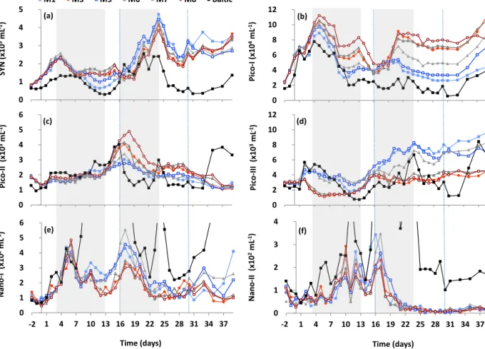
Figure 1. (a)Time series plot of depth-integrated (0.3–10 m) total phytoplankton abundance (<20 µm) and(b)total eukaryotic phytoplankton abundance for each mesocosm and the surrounding waters (Baltic). Dotted lines indicate the end of Phase I and the end of Phase II. Colours and symbols represent the different mesocosms and are consistent throughout the paper. MeanfCO₂during the experiment (days 1–43):

M1, 365 µatm; M3, 1007 µatm; M5, 368 µatm; M6, 821 µatm; M7, 497 µatm; M8, 1231 µatm.

were identified based on their divergence (Fig. 2). The first (NMDS-based period 1) followed the initial peak in abundance (days 3–13) with the highest abundances occurring in the elevated CO₂ mesocosms (Fig. 1a). During the second period (NMDS-based period 2; days 16–24), abundances were higher in the lowfCO₂mesocosms (Fig. 1a). In general the NMDS plot shows that throughout the experiment, mesocosm M1 followed the same basic trajectory as mesocosms M5 and M7, whilst mesocosm M3 followed M6 and M8 (Fig. 2). Thus, the two mesocosms (representing high and lowfCO2treatments) deviated from each other during Phase I and were clearly separated during Phases II and III (Fig. 2).

Phytoplankton abundances in the surrounding water started to differ from the mesocosms during Phase 0 (on average 44 % lower), which was primarily due to lower abundances of SYN. This effect was seen from day−1 prior to CO₂ addition but following bubbling with compressed air (day−5). On day 15, a deep mixing event occurred as a result of storm conditions (with consequent alterations in temperature and salinity). As a result phytoplankton abundances in the surrounding open water diverged more strongly from the mesocosms but remained similar in their dynamics (Fig. 3).

Microbial abundances in the 0–17 m samples were slightly

lower but showed very similar dynamics to those in the 0–

10 m samples (Fig. S1 in the Supplement).

3.1.1 Synechococcus

The prokaryotic cyanobacteria Synechococcus (SYN) accounted for the majority of total abundance, i.e. 74 % averaged across all mesocosms over the experimental period.

Abundances of SYN showed distinct variability between the different CO₂ treatments,starting on day 7, with the low CO₂ mesocosms exhibiting nearly 20 % lower abundances between days 11 and 15 compared to high fCO2 mesocosms (Fig. 3a). SYN net growth rates during days 3–13 (NMDS-based period 1) were positively correlated with CO2

(p=0.10,R²=0.53; Table 2, Fig. S2a). One explanation for higher net growth rates at elevated CO2could be the significantly (p <0.05) higher grazing rate in the low fCO₂ mesocosm M1 (0.56 d⁻¹) compared to the highfCO₂M3 (0.27 d⁻¹) as measured on day 10 (Fig. 4a). After day 16, SYN abundances increased in all mesocosms, and during this period (days 16–24) net growth rates had a significant negative correlation withfCO₂(p=0.05,R²=0.63; Figs. 3a and S3a, Table 2). Consequently, the net increase in SYN abundances during this period was on average 20 % higher at low fCO₂ compared to high fCO₂. This corresponded

(7)

Figure 2.Non-metric multidimensional scaling (NMDS) ordination plot of microbial community development in each mesocosm and the surrounding waters (Baltic) over the experimental period. Phases are indicated by different open symbols. Days of experiment (DoE) when communities separate (3, 13, 16 and 24) are indicated by different closed symbols. Phytoplankton groups are denoted as SYN (Syn), Pico-I (P-I), Pico-II (P-II), Pico-III (P-III), Nano-I (N-I), Nano-II (N-II), low NA prokaryotes (LNA) and high NA prokaryotes (HNA).

to higher total loss rates in high fCO2 treatments measured on day 17 (0.33 vs. 0.17 d⁻¹ for M3 and M1, respectively; Fig. 4a). The higher net growth most likely led to the peak in SYN abundance observed on day 24 (maximum 4.7×10⁵mL⁻¹), which was negatively correlated with fCO₂(p=0.01,R²=0.80; Table 3, Fig. S4a). After this period (days 24–28), SYN abundances declined at comparable rates in the different mesocosms irrespective of fCO₂ (Fig. 3a). Abundances in the low fCO₂ mesocosms remained higher into Phase III (Fig. 3a). SYN abundances in the surrounding water were generally lower than in the mesocosms, with the exception of days 17–21.

3.1.2 Picoeukaryotes

In contrast to the prokaryotic photoautotrophs, the eukaryotic phytoplankton community showed a strong positive response to elevated fCO2 (Fig. 1b). Pico-I was the numerically dominant group of eukaryotic phytoplankton, accounting for an average 21–26 % of total phytoplankton abundances. Net growth rates leading up to the first peak in abundance (from days 1 to 5) had a strong positive correlation withfCO₂(p <0.01,R²=0.90; Figs. 3b and S5a, Table 3).

Accordingly, the peak on day 5 (maximum 1.1×10⁵mL⁻¹; Fig. 3b) was also correlated positively withfCO₂(p=0.01, R²=0.81; Table 3, Fig. S4b). During Phase I from days 3 to 13 (i.e. NMDS-based period 1), net growth rates of Pico-I remained positively correlated with CO₂ concentration (p=0.01,R²=0.80; Table 2, Fig. S2b). However, during this period there was also a decline in abundance (days 5–9;p <0.01,R²=0.89; Table 3, Fig. S5b) with 23 % more

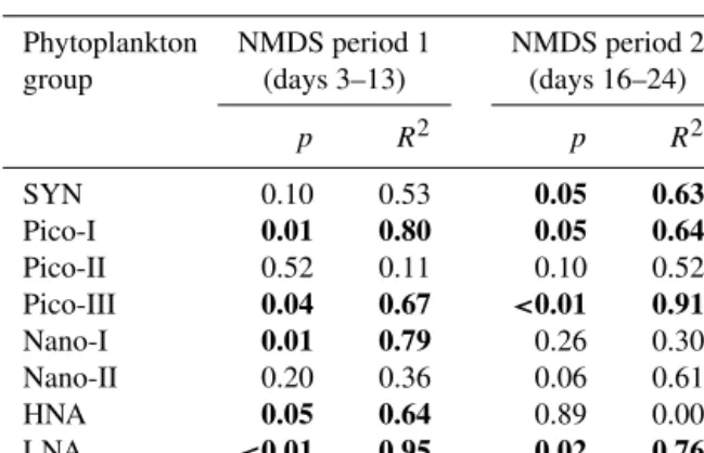
Table 2.The fit (R²) and significance (pvalue) of linear regressions applied to assess the relationship between net growth rate and temporally averagedfCO₂for the different microbial groups distinguished by flow cytometry. The results presented are for two periods distinguished from NMDS analysis: NMDS-based period 1 (days 3–13) and 2 (days 16–24). A significance level ofp≤0.05 was taken and significant results are shown in bold.

Phytoplankton NMDS period 1 NMDS period 2

group (days 3–13) (days 16–24)

p R² p R²

SYN 0.10 0.53 0.05 0.63

Pico-I 0.01 0.80 0.05 0.64

Pico-II 0.52 0.11 0.10 0.52

Pico-III 0.04 0.67 <0.01 0.91

Nano-I 0.01 0.79 0.26 0.30

Nano-II 0.20 0.36 0.06 0.61

HNA 0.05 0.64 0.89 0.00

LNA <0.01 0.95 0.02 0.76

cells lost in the lowfCO2mesocosms. Accordingly, following this period, gross growth rate was significantly higher in the highfCO₂ mesocosm M3 compared to the lowfCO₂ mesocosm M1 (day 10, p <0.05; Fig. 4b). Pico-I abundances in the surrounding open water started to deviate from the mesocosms after day 10 and were on average around half that of the lowfCO₂mesocosms (Fig. 3b). Following a brief increase (occurring between days 11 and 13) correlated with fCO₂(p <0.01,R²=0.94; Table 3, Fig. S4c), abundances declined sharply between days 13 and 16 (Fig. 3b), coincid-

(8)

0 1 2 3 4 5

SYN (x105 mL-1)

(a)

0 2 4 6 8 10 12

Pico-I (x104 mL-1) (b)

0 1 2 3 4 5 6

Pico-II (x103 mL-1) (c)

0 1 2 3 4 5 6

1 4 7 10 13 16 19 22 25 28 31 34 37 Nano-I (x102 mL-1)

Time (days) (e)

-2

0 2 4 6 8 10 12

Pico-III (x103 mL-1) (d)

0 1 2 3 4

1 4 7 10 13 16 19 22 25 28 31 34 37 Nano-II (x102 mL-1)

Time (days) (f)

-2

Figure 3.

Figure 3.Time series plot of depth-integrated (0.3–10 m) abundances of(a)Synechococcus(SYN),(b)picoeukaryotes I (Pico-I),(c)picoeukaryotes II (Pico-II),(d)picoeukaryotes III (Pico-III),(e)nanoeukaryotes I (Nano-I) and(f)nanoeukaryotes II (Nano-II) distinguished by flow cytometric analysis of the microbial community in each mesocosm and the surrounding waters (Baltic). Dotted lines indicate the end of Phase I and the end of Phase II; grey areas indicate NMDS-based periods 1 and 2 during which net growth rates were analysed.

Table 3.The fit (R²) and significance (pvalue) of linear regressions used to relate peak abundances and net growth rate with temporally averagedfCO₂for the different microbial groups distinguished by flow cytometry during specific periods of interest. A significance level ofp≤0.05 was taken and significant results are shown in the table below.

Peak abundance Net growth rate

p R² p R²

SYN day 24 0.01 0.80 – –

Pico-I day 5 0.01 0.81 – –

Pico-I day 13 <0.01 0.94 – –

Pico-I day 21 0.01 0.84 – –

Pico-II day 17 <0.01 0.93 – –

Pico-III day 24 <0.01 0.91 – –

Nano-I day 17 0.04 0.67 – –

Pico-I days 1–5 – – <0.01 0.90

Pico-I days 5–9 – – <0.01 0.89

Pico-II days 12–17 – – 0.01 0.82

ing with a significantly higher total mortality rate in the high fCO₂mesocosm M3 (day 13; Fig. 4b). Viral lysis was a sub- stantial loss factor relative to grazing for this group, com- prising an average 45 and 70 % of total losses in M1 and M3, respectively (Table S1). During NMDS-based period 2, net growth rates of Pico-I were significantly higher at high fCO₂(p=0.05,R²=0.64; Table 2, Fig. S3b). By day 21, abundances in the highfCO₂mesocosms were (on average)

∼2-fold higher than at low fCO₂ (maximum abundances 8.7×10⁴and 5.9×10⁴mL⁻¹for high and lowfCO2meso- cosms;p=0.01, R²=0.84; Table 3, Fig. S4d). Standing stock of Pico-I remained high in the elevatedfCO2 mesocosms for the remainder of the experiment (7.9×10⁴ vs.

4.3×10⁴mL⁻¹ on average for high and lowfCO2 mesocosms, respectively; Fig. 3b). Additionally, gross growth rates during this final period were relatively low (0.14 and 0.16 d⁻¹in M1 and M3, respectively) and comparable to total loss rates (averaging 0.13 and 0.10 d⁻¹over days 25–31 for M1 and M3, respectively; Fig. 4b).

Another picoeukaryote group, Pico-II, slowly increased in abundance until day 13, when it increased more rapidly

(9)

*

0 0.2 0.4 0.6

SYN rate (d-1)

Total loss M1 Total loss M3 Gross growth M1 Gross growth M3

(a)

*

* * *

*

0 0.2 0.4 0.6

Pico-I rate (d-1) (b)

*

0 0.2 0.4 0.6 0.8 1

Pico-II rate (d-1) (c)

* 0

0.2 0.4 0.6 0.8 1

1 3 6 10 13 17 20 24 31

Nano-I rate (d-1)

Day number (e)

* 0 0 0 0

0.2 0.4 0.6 0.8 1 1.2 1.4

1 3 6 10 13 17 20 24 31

Nano-II rate (d-1)

Day number (f)

* * *

0 0

*

* 0

0.2 0.4 0.6 0.8 1

Pico-III rate (d-1) (d)

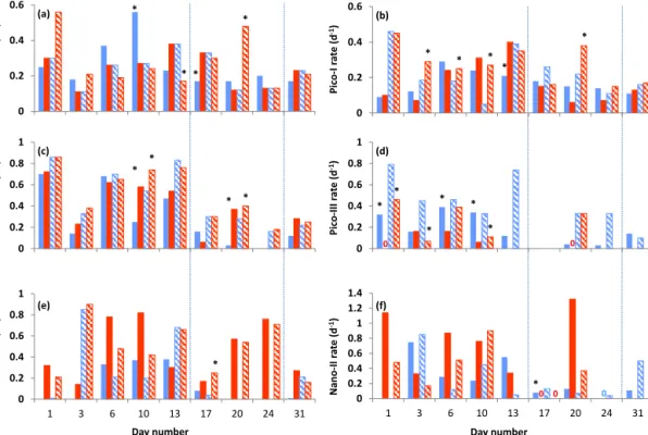
Figure 4.Total mortality rates (i.e. grazing and lysis; solid bars) and gross growth rates (striped bars) d⁻¹of the different phytoplankton groups in mesocosms M1 (blue) and M3 (red) on the day indicated:(a)Synechococcus(SYN),(b)picoeukaryotes I (Pico-I),(c)picoeukaryotes II (Pico-II),(d)picoeukaryotes III (Pico-III),(e)nanoeukaryotes I (Nano-I) and(f)nanoeukaryotes II (Nano-II). Significant (p≤0.05) differences between mesocosms are indicated by an asterisk above the relevant bar (either total loss or gross growth). A coloured zero indicates that a rate of zero was measured in the mesocosm of the corresponding colour; the absence of a bar or zero indicates a failed experiment.

Dotted lines indicate the end of Phase I and the end of Phase II.

(Fig. 3c). Gross growth rates measured during Phase I were high (0.69 and 0.72 d⁻¹on average in the low and highfCO₂ mesocosms M1 and M3, respectively; Fig. 4c) and comparable to loss processes (0.46 and 0.58 d⁻¹), indicative of a relatively high turnover rate of production. Overall net growth rates during days 3–13 (NMDS-based period 1) did not cor- relate with CO₂ (p=0.52, R²=0.11; Table 2, Fig. S2c).

However, during periods of rapid increases in net growth, abundances were positively correlated with CO2concentra- tion (days 12–17; p=0.01,R²=0.82; Table 3, Fig. S5c).

Accordingly, the peak in abundances of Pico-II on day 17 displayed a distinct positive correlation withfCO2(p <0.01, R²=0.93; Table 3, Fig. S4e) with maximum abundances of 4.6×10³ and 3.4×10³mL⁻¹ for the high and lowfCO₂ mesocosms, respectively (Fig. 3c). In M8 (the highestfCO₂ mesocosm), abundances increased for an extra day with the peak occurring on day 18, resulting in an average of 23 % higher abundances. During the decline in the Pico-II peak (days 16–24), net growth rates were negatively correlated withfCO₂(p=0.10,R²=0.52; Table 2, Fig. S3c). More- over, the rate of decline was faster for the highfCO₂mesocosms during days 18–21 (p <0.01,R²=0.85). The Pico-II abundances in the surrounding water were comparable to the

mesocosms during Phases 0 and I, lower during Phase II and higher during Phase III (Fig. 3c).

Pico-III exhibited a short initial increase in abundances in the lowfCO₂treatments, resulting in nearly 2-fold higher abundances at low fCO₂ by day 3 compared to the high fCO₂ treatment (Fig. 3d). After this initial period, net growth rates of this group had a significant positive correlation with fCO2 (days 3–13; p=0.04,R²=0.67; Ta- ble 2, Fig. S2d). In general, during Phase I gross growth (p <0.01; days 1, 3, 10; Fig. 4d) and total mortality (p <

0.05; days 1, 6, 10; Fig. 4d) were significantly higher in the lowfCO2mesocosm M1 compared to the highfCO2meso- cosm M3, resulting in low net growth rates. During Phase II (days 16–24; NMDS-based period 2) the opposite occurred;

i.e. net growth rates were negatively correlated withfCO₂ (p <0.01,R²=0.86; Table 2, Fig. S3d). Maximum Pico-III abundances (day 24: 4.2×10³and 8.3×10³mL⁻¹for high and lowfCO₂) had a strong negative correlation withfCO₂ (p <0.01, R²=0.91; Table 3, Fig. S4f). Pico-III abundances remained noticeably higher in the lowfCO₂ mesocosms during Phases II and III (on average 80 %; Fig. 3d).

Unfortunately, almost half of the mortality assays in this second half of the experiment failed (see Sect. 2), but the suc- cessful assays suggest that losses were minor (<0.15 d⁻¹;

(10)

Fig. 4d) and primarily due to grazing, as no significant viral lysis was detected (Table S1).

3.1.3 Nanoeukaryotes

Nano-I showed maximum abundances (4.3±0.4×10²mL⁻¹) on day 6 (except M1, which peaked on day 5) independent of fCO₂(p=0.23,R²=0.33; Fig. 3e). There was, however, a negative correlation of net growth rate with fCO₂ during days 3–13 (NMDS-based period 1;p=0.01,R²=0.79;

Table 2, Fig. S2e). A second major peak in abundance of Nano-I occurred on day 17, with markedly higher numbers in the lowfCO2mesocosms (4.1×10²mL⁻¹compared to 2.4×10²mL⁻¹in highfCO2mesocosms;p=0.04,R²= 0.67; Figs. 3e and S4g, Table 3). Total loss rates in the high fCO2mesocosm M3 on days 6 and 10 were 2.3-fold higher compared to the lowfCO₂mesocosm M1 (Fig. 4e), which may help to explain this discrepancy in total abundance between low and highfCO₂mesocosms. Viral lysis accounted for up to 98 % of total losses in the highfCO₂mesocosm M3 during this period, whilst in M1 viral lysis was only detected on day 13 (Table S1 in the Supplement). Peak abundances (around 5.0×10²mL⁻¹) were much lower compared to those in the surrounding waters (max∼2.4×10³mL⁻¹; Figs. 3e and S6a). During Phase II, Nano-I abundances in the surrounding waters displayed rather erratic dynamics compared to those of the mesocosms but converged during certain periods (e.g. days 19–22). No significant relationship was found between net loss rates and fCO2 for the second NMDS- based period (p=0.26,R²=0.30; Table 2, Fig. S3e). At the end of Phase II, abundances were similar in all mesocosms but diverged again during Phase III (days 31–39) due primarily to a negative effect of CO₂on Nano-I abundances, as depicted in the average 36 % reduction in Nano-I.

The temporal dynamics of Nano-II, the least abundant phytoplankton group analysed in our study, displayed the largest variability (Fig. 3f), perhaps due to the spread of this cluster in flow cytographs (which may indicate that this group represents several different phytoplankton species).

No significant relationship was found between net growth rate andfCO₂for this group for the two NMDS-based periods (Table 2, Figs. S2f and S3f) nor with the peak in abundances on day 17 (p=0.13, R²=0.46; Fig. S4h). More- over, no consistent trend was detected in mortality rates (Fig. 4f). Similar to Nano-I, abundances in the surrounding water were often higher than in the mesocosms (maximum 3.5×10²mL⁻¹ vs. 1.1×10⁴mL⁻¹, respectively; Figs. 3f and S6b).

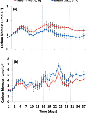
3.1.4 Algal carbon biomass

The mean combined biomass of Pico-I and Pico-II showed a strong positive correlation withfCO₂throughout the experiment (p <0.05,R²=0.95; Fig. 5a), an effect already noticeable by day 2. Their biomass in the highfCO₂meso-

0 1 2 3

Carbon biomass (µmol L-1)

Mean (M3, 6, 8) Mean (M1, 5, 7)

0 1 2 3 4 5 6 7 8

1 4 7 10 13 16 19 22 25 28 31 34 37 Carbon biomass (µmol L-1)

Time (days) (b)

-2 (a)

Figure 5. Time series plot of the mean phytoplankton carbon biomass in highfCO₂ (M3, M6, M8; red) and lowfCO₂ (M1, M5, M7; blue) mesocosms of (a) Pico-I and Pico-II combined and(b)SYN, Pico III, Nano-I and Nano-II combined. Error bars represent 1 standard deviation from the mean. Carbon biomass is calculated assuming a spherical diameter equivalent to the mean average cell diameters for each group and conversion factors of 237 fg C µm⁻³(Worden et al., 2004) and 196.5 fg C µm⁻³(Garri- son et al., 2000) for pico- and nano-sized plankton, respectively.

Dotted lines indicate the end of Phase I and the end of Phase II.

cosms was, on average 11 % higher than in the lowfCO2

mesocosms between days 10 and 20 and 20 % higher between days 20 and 39. Conversely, the remaining algal groups showed an average 10 % reduction in carbon biomass at enhancedfCO2 (days 3–39, the sum of SYN, Pico-III, Nano-I and II;p <0.01; Fig. 5b). The most notable response was found for the biomass of Pico-III, which showed an im- mediate negative response to CO₂ addition (Fig. S7a) and remained on average 29 % lower throughout the study period (days 2–39). For Nano-I and Nano-II the lower carbon biomass only became apparent during the end of Phase I and the beginning of Phase II (days 14–20; Fig. S7b). Due to its small cell size, the numerically dominant SYN accounted for an average of 40 % of total carbon biomass.

(11)

0 1 2 3 4 5

Prokaryotes (x106 mL-1)

(a)

0 1 2 3

HNA prok (x106 mL-1)

0 1 2 3

1 4 7 10 13 16 19 22 25 28 31 34 37 LNA prok (x106 mL-1)

Time (days) (c)

0 2 4 6 8 10

1 4 7 10 13 16 19 22 25 28 31 34 37 Total virus (x107 mL-1)

Time (days) (d)

-2 (b)

-2

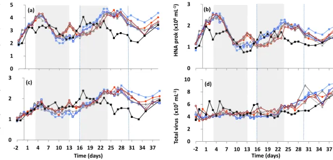
Figure 6.Time series plot of depth-integrated (0.3–10 m) abundances of(a)total prokaryotes,(b)high fluorescent nucleic acid prokaryote population (HNA),(c)low fluorescent nucleic acid prokaryote population (LNA) and(d)total virus. Dotted lines indicate the end of Phase I and the end of Phase II; grey areas indicate NMDS-based periods during which net growth rates were analysed.

* *

*

0 0.1 0.2 0.3 0.4 0.5 0.6

-3 0 4 7 11 14 18 21

Grazing rate (d-1)

Day number (a)

0 4 8 12 16 20

-3 0 4 7 11 14 18 21 25

% bacterial ss lysed (d-1)

Day number (b)

Figure 7.Prokaryote mortality rates:(a)total grazing (d⁻¹) and(b)viral lysis rates as % of prokaryote standing stock in mesocosms M1 (lowfCO₂; blue) and M3 (highfCO₂; red). Grazing rates were determined from fluorescently labelled prey, and viral lysis rates from viral production assays. Error bars represent 1 standard deviation of triplicate assays. Significant (p≤0.05) differences between mesocosms are indicated by an asterisk. Dotted lines indicate the end of Phase I.

3.2 Prokaryote and virus population dynamics

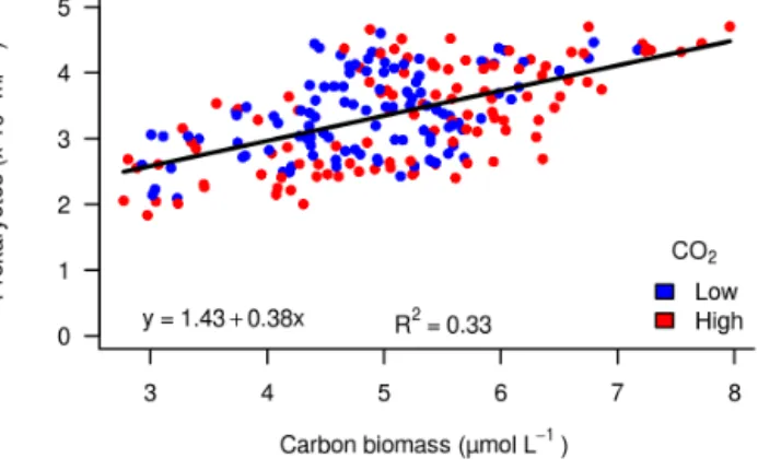
Prokaryote abundance in the mesocosms was positively re- lated to total algal biomass independent of treatment (p <

0.05,R²=0.33; Fig. 8) and generally followed total algal biomass (Fig. S7c). The initial increase in total prokaryote abundances occurred during the first few days following the closure of the mesocosms (Fig. 6a). This was primarily due to increases in the HNA prokaryote group (Fig. 6b), which displayed higher net growth rates (0.22 d⁻¹) compared to the LNA prokaryotes (0.14 d⁻¹ on days −3 to 3; Fig. 6c). A similar, albeit somewhat lower, increase was also recorded in the surrounding waters (Fig. 6a). The decline in the first peak in prokaryote abundances coincided with the decay in phytoplankton abundance and biomass (Figs. 1a and S7c).

Concurrently the share of viral lysis increased, representing 37–39 % of total mortality on day 11 (Fig. 7b). No measur-

able rates of lysogeny were found for the prokaryotic community during the experimental period (all phases). From days 10 to 15 prokaryote dynamics (total, HNA and LNA) became noticeably affected by CO2concentration with a significant positive correlation between net growth andfCO2

during Phase I (days 3–13; NMDS-based period 1; Table 2, Fig. S2g and h). In the higherfCO₂mesocosms, the decline in prokaryote abundance occurring between days 13 and 16 (Fig. 6a) was largely (70 %) due to decreasing HNA prokaryote numbers (Fig. 6b). The grazing was 1.6-fold higher in the highfCO₂mesocosm M3 compared to M1 (0.36±0.13 and 0.14±0.08 d⁻¹on day 14; Fig. 7a). At the same time, viral abundance increased in the highfCO₂mesocosms (Fig. 6d).

During Phase II, prokaryote abundances increased steadily until day 24 (for both HNA and LNA), corresponding to increased algal biomass (Figs. 6 and S7c) and lowered grazing rates (Fig. 7a). Specifically, during days 16–24 (NMDS-

(12)

Figure 8.Correlation between total carbon biomass (µmol L⁻¹) and total prokaryote abundance in lowfCO₂mesocosms (M1, M5, M7;

blue) and highfCO₂mesocosms (M3, M6, M8; red) throughout the experiment (days−2 to 39).

based period 2), the HNA prokaryotes showed an average 10 % higher abundances in the low compared to the high fCO₂mesocosms (Fig. 6b). However, a significant negative correlation of net growth rates and fCO₂ was only found for LNA (Table 2, Fig. S3g and h). No significant differences in loss rates between M1 and M3 were found during Phase II (p=0.22 and p=0.46 on days 18 and 21, respectively; Fig. 7). Halfway through Phase II (day 24), the prokaryote abundance in the surrounding water levelled off (Fig. 6a). Prokaryote abundance ultimately declined during days 28–35 (Fig. 6a), and the net growth of LNA was again negatively correlated with enhanced CO2 (p=0.02, R²=0.76; Table 2, Fig. S3g). Unfortunately, no experimental data on grazing and lysis of prokaryotes are present after day 25. However, viral abundances increased steadily at 2.2×10⁶d⁻¹concomitant with a decline in prokaryote abundance (Fig. 6a and d). There was no significant correlation between viral abundances andfCO₂during Phases II and III (p=0.36,R²=0.21).

4 Discussion

In most experimental mesocosm studies, nutrients have been added to stimulate phytoplankton growth (Schulz et al., 2017); therefore limited data exists for oligotrophic phytoplankton communities. In this study, we describe the impact of increased fCO2 on the brackish Baltic Sea microbial community during summer (nutrient depleted; Paul et al., 2015). Small-sized phytoplankton numerically dominated the autotrophic community, in particular SYN and Pico-I (both about 1 µm in cell diameter). Our results demonstrate variable effects of fCO₂ manipulation on temporal phytoplankton dynamics, dependent on phytoplankton group. In particular, Pico-I and Pico-II showed significant positive responses, whilst the abundances of Pico-III, SYN and Nano-I were negatively influenced by elevated fCO₂.

The impact of OA on the different groups was, at times, a direct consequence of alterations in gross growth rate, whilst overall phytoplankton population dynamics could be explained by the combination of growth and losses. OA effects on community composition in these systems may have consequences on both the food web and biogeochemical cycling.

4.1 Comparison with surrounding waters

During Phase 0, the microbial assemblage showed good replicability among all mesocosms; however, they had already began to deviate from the community in the surrounding waters. This was most likely a consequence of water movement altering the physical conditions and biological composition of the surrounding water body. The dynamic nature of water movement in this region has been shown to alter the entire phytoplankton community several times over within a few months due to fluctuations in nutrient supply, advection, replacement or mixing of water masses and water temperature (Lips and Lips, 2010). Alternatively, the effects of enclosure and the techniques (bubbling) used to ensure a homogenous water column may have stimulated SYN within the mesocosms, which has been found to occur in several mesocosm experiments (Paulino et al., 2008;

Gazeau et al., 2017). By Phases II and III, the microbial abundances within the mesocosms were distinctly different from the surrounding waters, with generally fewer SYN and Pico-I and more Nano-I and Nano-II. Our statistical analysis shows that during this time, there was little similarity between the surrounding waters and mesocosms regardless of the CO₂treatment level. Thus, the deviations during this time were most likely due to an upwelling event in the archipelago (days 17–30; Paul et al., 2015). Cold, nutrient-rich deep water has been shown to upwell during summer with a pro- found positive influence on ecosystem productivity (Nôm- mann et al., 1991; Lehmann and Myrberg, 2008). A relax- ation from nutrient limitation in vertically stratified waters disproportionately favours larger-sized phytoplankton due to their higher nutrient requirements and lower capacity to com- pete at low concentrations dictated by their lower surface to volume ratio (Raven, 1998; Veldhuis et al., 2005). Inside the mesocosms, which were isolated from upwelled nutrients, picoeukaryotes dominated similar to a stratified water column.

Following this upwelling event, the pH of the surrounding waters dropped from 8.3 to 7.8, a level comparable to the highest CO₂ treatment (M8) on day 32 (Paul et al., 2015).

This suggests that other factors contributed to the observed differences between mesocosms and the surrounding water than can be accounted for by CO₂concentration alone, e.g.

nutrients. Alternatively, the magnitude and source of mortality occurring in the surrounding water may have been altered compared to within the mesocosms after such an upwelling event. Although the grazer community in the surrounding waters was not studied during this campaign, it is likely that

2 f CO :amesocosmstudyintheeasternBalticSea Alterationsinmicrobialcommunitycompositionwithincreasing

Alterations in microbial community composition with increasing f CO 2 : a mesocosm study in the eastern Baltic Sea

Alterations in microbial community composition with increasing f CO ₂ : a mesocosm study in the eastern Baltic Sea