Decision Bounds for Data-Admissible Seasonal Models

November 1997

Decision Bounds for Data-Admissible Seasonal Models

Robert M. Kunst

Robert M. Kunst Title:

Decision Bounds for Data-Admissible Seasonal Models ISSN: Unspecified

1997 Institut für Höhere Studien - Institute for Advanced Studies (IHS) Josefstädter Straße 39, A-1080 Wien

E-Mail: o ce@ihs.ac.atffi Web: ww w .ihs.ac. a t

All IHS Working Papers are available online: http://irihs. ihs. ac.at/view/ihs_series/

This paper is available for download without charge at:

https://irihs.ihs.ac.at/id/eprint/1029/

Institute for Advanced Studies, Vienna

Reihe Ökonomie / Economics Series No. 51

Decision Bounds for Data-Admissible Seasonal Models

Robert M. Kunst

Seasonal Models

Robert M. Kunst

Reihe Ökonomie / Economics Series No. 51

November 1997

Robert Kunst

Institut für Höhere Studien Stumpergasse 56, A -1060 Wien Phone: +43/1/599 91-255 Fax: +43/1/599 91-163 e-mail: kunst@ihs.ac.at and

Johannes Kepler University Linz

Institut für Höhere Studien (IHS), Wien

Institute for Advanced Studies, Vienna

The Institute for Advanced Studies in Vienna is an independent center of postgraduate training and research in the social sciences. The Economics Series presents research done at the Economics Department of the Institute for Advanced Studies. Department members, guests, visitors, and other researchers are invited to contribute and to submit manuscripts to the editors. All papers are subjected to an internal refereeing process.

Editorial Main Editor:

Robert M. Kunst (Econometrics) Associate Editors:

Walter Fisher (Macroeconomics) Arno Riedl (Microeconomics)

The selection problem among models for the seasonal behavior in time series is considered.

The central decision of interest is between models with seasonal unit roots and with deterministic cycles. In multivariate models, also the number of stochastic seasonal factors is a discrete parameter of interest. To enable restricting attention to data-admissible models, a new attempt is made at defining data admissibility. Among data-admissible model classes, statistical decision rules are constructed on the basis of weighting priors and decision-bounds analysis. The procedure is applied to some exemplary economics series. Many univariate series select models without seasonal unit roots but the bivariate experiments enhance the importance of seasonal unit roots with restricted influence of seasonal constants. The framework of decision-bounds analysis offers a convenient alternative to sequences of classical hypothesis tests.

Keywords

Unit roots, seasonal cointegration, model selection

JEL-Classifications

C32

1 Introduction

For a long time, seasonal characteristics of economic series were viewed as being resid- ual and without inherent economic interest. The usual practice was to focus on de- seasonalized data, at least in the eld of macroeconomics. Typically, de-seasonalization was achieved by the application of seasonal adjustment lters. However, recently the drawbacks of this practice and the possible economic relevance of seasonality have been fully recognized. Many economists have realized, rstly, that the supposedly seasonal noise part of the series contains important information about the non-seasonal com- ponent and, secondly, that the seasonal component of one series contains information about the seasonal and non-seasonal components of other series. In short, any attempt to decompose the world of economics into two mutually independent worlds, one being non-seasonal and of economic interest and the other one being seasonal and uninterest- ing, is misguided. A good survey of the historical developments that led to the modern econometrics of seasonality can be found in Hylleberg (1992).

The need to view the whole of the economic variable of interest within a full model that incorporates seasonal features as well as trend and business cycle characteris- tics has instigated the development of various seasonal time series models. Building on the traditional low-order autoregressive (AR) model, which is a convenient rst- order approximation to the dynamic properties of most time series in the absence of a theoretical model, three ways have been used repeatedly in order to capture seasonal characteristics. Firstly, seasonal constants can be added to the deterministic part of the model. These seasonal-dummy models are characterized by inexible and repetitive cy- cles and by predictions that are mainly projections of the average in-sample cycle into the future. Secondly, stable conjugate complex roots in the AR polynomial may reect non-persistent seasonality. Thirdly, seasonal unit roots have been suggested by Hylle- berg et al. (1990) and others to allow permanent shifts in the seasonal structure.

These models with non-stationary stochastic seasonality are characterized by exible and shape-changing cycles and by predictions that mainly project the present shape of the seasonal cycle into the future, with a low degree of predictive precision due to the non-stationarity. Amalgams of these models have also been used but we will point to some of their drawbacks in this paper.

This apparent variety of available models calls for an ecient model selection strat-

egy. In this paper a framework for a multiple decision strategy with regard to model

selection is developed. The basic choice set of seasonal models is determined by argu-

ments of data admissibility, as we feel that one should be suspicious of models that are

not data-admissible. The concept of data admissibility permits to impose plausibility

restrictions on process trajectories and to discard models that have a high probability

of generating implausible trajectories. Following the exclusion of non-admissible mod- els from consideration, the choice among the remaining candidates is often guided by sequences of hypothesis tests, whereas other researchers use Bayesian methods. This paper introduces a multiple decision (MD) strategy as a third alternative that builds on Bayesian ideas but assigns a central position to a loss function that is designed to penalize certain mismatches between selected and true model harder than others. The elicitation of weighting priors within each model class is guided by the idea of uni- form distributions over bounded regions of parameter values. A similar approach was followed by Franses et al. (1997) for certain seasonal processes in a fully Bayesian setting. However, the present work diers in two main aspects. Firstly, for our bivariate experiments we use uniform weighting on eigenvalues and not on the coecient space.

Secondly, we form decision rules by loss functions.

The remainder of this paper is organized as follows. A step toward a more rigorous denition of data admissibility is taken in Section 2. In Section 3 existing seasonal models are reviewed under the aspect of data admissibility. Section 4 concentrates on constructing multiple decision bounds in order to permit an ecient selection among competing models. In Section 5, empirical applications to some macroeconomic series are reported. We robustify the results by also reporting some sensitivity experiments.

Section 6 concludes. An appendix expounds the basics of the multiple decisions tech- nique used in this paper.

2 The concept of data admissibility

The reference work by Hendry (1995, p.364) gives the following verbal denition of data admissibility:

"A model is data admissible if its predictions automatically satisfy all known data constraints."

In this denition, a correct interpretation of the word `prediction' appears to be crucial.

If it stands for point prediction from the realized sample | or possibly subsamples

thereof | by means of conditional expectation, the denition may appear slightly too

liberal for empirical applications. For example, consider three models: (a) white noise

plus a constant a ; (b) a random walk started from the value a ; (c) some nonlinear

but symmetric generating law that also starts from a but is stationary only in a local

neighborhood of a and is explosive otherwise. All three models result in the same

conditional-expectation point forecast a . However, we feel that for a naturally bounded

economic variable only model (a) is admissible, whereas for an unbounded variable we

may also accept model (b) but not (c).

On the other hand, if `prediction' means the predictor process in its interpretation as a random variable, though possibly conditioned on some starting values in the data sample, the denition is very restrictive. We formalize the two extreme interpretations in two tentative denitions. We remark that, as we are concerned with models for time series, we view `models' as parametric collections of time-series processes.

Denition1

. A process is called data-admissible in mean prediction if none of its point forecasts at any step size dened by conditional expectations from observed samples or subsamples thereof violates logical constraints. A model parameterized by a param- eter

is called data-admissible in mean prediction if all

dene admissible processes.

The dened property is sample-dependent. It is conceivable that we construct an arti- cial sample that is close but not identical to the observed one, apply the model under investigation with a certain xed value of , and violate the logical constraints for a certain step size. The following alternative denition marks the other extreme.

Denition 2.

A process is called strictly data-admissible if it is conceivable as a data- generating mechanism for the observed n-dimensional economic variable for all t

I , where I is the index time range for the considered class of time-series processes. Typ- ically, I =

. A parametric model is called strictly data-admissible if all

dene data-admissible processes.

Verbal elements such as `logical constraints' and `conceivable' are intended to leave room for expert evaluation by economic theorists. Some logical constraints are certain or almost sure, such as denitional identities, but for others their violation is just extremely unlikely. Under the latter category come e.g. trajectories for unemployment rates that remain at a level beyond 90% for several decades, under the former category come trajectories with unemployment rates outside the range [0,1]. Practical usage of the denition requires the assumption of a set of conditions

which conceivable trajectories are not allowed to violate.

could exclude impossible values but also other features, such as disproportionate growth, explosive cycles, or sudden jumps. In the following, we will use as sets

interval restrictions to avoid impossible values or cone- type restrictions to avoid excessive expansion from starting values.

We note that, e.g., the model of Brownian motion is not strictly data-admissible for the

unemployment rate as almost every trajectory of its processes crosses the boundaries

of 0 and 1, even if started from real-life values. The same is probably true for many

economic and econometric models used in practice. However, an economist may feel

quite comfortable with such models for a certain time span and may be willing to use

them to explain the local behavior of economic variables that are strictly bounded. One

may consider to replace Denition 2 by a `local' denition requiring the admissibility

constraints to just hold for a limited part of the time range I . However, then the plausibility of the analysis depends on the life span of trajectories that may be quite low. It makes more sense to exploit the LIL (law of the iterated logarithm) property of the random walk which guarantees that generated trajectories violate certain prescribed boundaries at most nitely often. We introduce the following denition for weak-sense data admissibility, which is stronger than Denition 1 but weaker than Denition 2 and may be able to capture the properties that are interesting in practice.

Denition3

. A process is called (weak-sense) data-admissible if its trajectories violate bounds constructed from plausibility arguments at most nitely often. A model is called (weak-sense) data-admissible if all

dene data-admissible processes.

Clearly, a strictly data-admissible model is data-admissible. A data-admissible model is admissible in mean prediction unless the observed sample has been created from the nite number of constraint violations. The characteristic properties of Denition 3 are seen as follows. Suppose the admissibility bounds are dened by some function g ( t ) such that

=

X

[ X 0 + at

g ( t ) ;X 0 + at + g ( t )]

. We assume that (a) g (0) > 0, (b) g ( t ) increases monotonously in t , (c) lim

g ( t ) = log t =

and hence also lim

g ( t ) =

, (d) lim

g ( t ) =t = 0. In short, g ( t ) is sublinear but grows faster than log t . We note that, assuming a > 0 and X 0 > 0, this admissibility condition is stricter than

=

X

> 0

, i.e. positivity of trajectories. The `trend-stationary' model X

= X 0 + at + "

with Gaussian white noise "

is certainly data-admissible in mean prediction.

However, it is also weak-sense admissible due to the extremal properties of the Gaussian distribution, though it can never attain strict admissibility due to the unboundedness of the support of the Gaussian law. Due to the LIL, the drifting random walk started from X 0 and with drift constant a is also a weak-sense data-admissible model. If the drift is unknown, widening

to e.g.

=

X

[ X 0 + a 1 t

g ( t ) ;X 0 + a 2 t + g ( t )]

with 0 < a 1 < a 2 will result in data-admissible drifting random walks over a useful range of drift parameters, such that we can hope that the sample estimate falls into the prescribed range [ a 1 ;a 2 ]. In contrast, all models with disproportionate growth, such as X

= X

1 + a + bt + "

, are clearly inadmissible.

3 Seasonal time series models

In the following, we will use the conventional time-series abbreviations, such as B for

the lag operator, i.e. X

1 = BX

, for rst dierences 1

B , and 4 = 1

B ⁴ for

seasonal dierences. Without undue lack of generality, we will concentrate on the case

of quarterly data throughout. We will use "

to denote a white-noise series. Wherever

we need stronger properties, we will tacitly also assume that "

is Gaussian white noise.

For exposition, we rst consider the seasonal time series model 4 X

=

⁴

i

=1

D

+ "

(1) D

are seasonal constants that 1 in the i {th quarter and 0 in the other quarters. The deterministic part of the right-hand side admits some alternative equivalent represen- tations:

4

X

i

=1

D

= +

³

i

=1

D

= + a cos( t ) + b cos( t

2 ) + c cos( ( t

1) 2 )

There is an obvious one-one mapping between the three representations in the param- eters ( 1 ;:::; 4 ), ( ;

₁ ; ₂

;

₃ ), and ( ;a;b;c ).

The model (1) is an amalgam of two popular time series models, the seasonal random walk with drift

4 X

= a + "

; (2)

and the random walk with seasonally varying drift X

=

⁴

i

=1

D

+ "

: (3) These models have been repeatedly used in the econometric literature to describe the behavior of seasonal data. To capture the serial correlation in the errors, they are usually `augmented' with autoregressive lags of the left-hand-side variable, such as

P

p;

4

i

=1 '

4 X

for cases (1) and (2). Our point is that the two simpler models (2) and (3) are data-admissible with respect to a plausible set

but that the amalgam model (1) is not data-admissible. In particular we dene the admissibility set

by

A

=

max

i

4

X

X

< g ( t )

(4) with the function g ( t ) obeying the restrictions lim

g ( t ) = log t =

and lim

g ( t ) =t = 0 as motivated in the last section. If m

denotes the maximum dierence

, additional conditions such as g (0) > m

and g ( t ) dierentiable with g

( t ) > 0 exclude uninteresting cases. Note that

is designed to contain secular expansion ( i = 4) as well as intra-annual seasonal expansion ( i < 4).

The process (1) is composed of four interspersed random walks with dierent drift constants. The dierence of two of these four random walks with drift dierence m

is again a random walk Z

with drift proportional to m

. Because of the law of the iterated logarithm (LIL)

lim

t!1

sup Z

m

t

(2 t log log t ) ¹

² = 1 a.s. (5)

(see, e.g., Davidson, 1994, p.408), the set

is violated by the process with probability one. Note that even the deterministic skeleton of the model violates

for t large enough.

The average life span strictly decreases with m

and can be quite low for empirically relevant parameter combinations.

In contrast, for (2) the dierence X

X

is a random walk with zero drift. It follows from the LIL that

will only be violated for nitely many t as g ( t ) was assumed to grow faster than the denominator in (5). Hence, the model (2) is weak-sense data- admissible. For (3), the dierences Z

= X

X

are bounded in probability. The maximum of the Z

is essentially governed by c log t and the Gumbel distribution (cf.

Johnson and Kotz , 1970, p.276). It follows that (3) is not strictly admissible due to the unbounded support of the increments but that the model is weak-sense admissible if g ( t ) grows faster than log t . The problem evolves how then to reconcile the two ideas of deterministic and stochastic seasonality in (2) and (3) in one comprehensive model and retain the property of weak-sense data admissibility. The answer is that this is not possible for univariate X . If one really wants to include deterministic seasonality within the framework of seasonal unit roots, this can only be done by allowing for a seasonal starting pattern or by considering dierent, more complicated, structures. However, for multivariate X , such a reconciliation is possible.

A class of multivariate seasonal models with univariate marginal models of the admis- sible type (2) was suggested recently by Franses and Kunst (1996) who consider special restrictions on seasonally cointegrated models. We use the following additional notational conventions. 2 denotes the second-order dierencing operator 1

B ² , S ( B ) is the seasonal moving average 1 + B + B ² + B ³ , A ( B ) is the moving average with al- ternating signs 1

B + B ²

B ³ . Note that these three operators are factors of the seasonal dierencing operator 4 . In this notation, the n -dimensional seasonal model considered by Franses and Kunst reads

4 X

= 1 ₁

S ( B ) X

1 + 2 ( ₂

A ( B ) X

1 + a

cos ( t

1)) + 3

₃ 2 X

2 + ( b

;c

)(cos

2( t

1) ; cos

2( t

2))

+ +

⁴

i

=1

4 X

+ "

(6)

The dimensionalities are n

r

for

and

, i = 1 ; 2 ; 3, r 2

1 for a

, r 3

1 for b

and c

, and n

n for the

matrices. The model allows for a non-zero general drift and also for deterministic seasonal inuences 2 a

and 3 ( b

;c

) at the frequencies and = 2.

These are proportional to the loading vectors of the seasonal error-correcting structures.

Hence, the coecients a;b;c of the regressors cos( t

1) ; cos( t

1) = 2 ; cos( t

2) = 2

are restricted by a = 2 a

;b = 3 b

;c = 3 c

. These parameter restrictions cannot be expressed conveniently in the representation with coecients

;i = 1 ;:::; 4 and the regressors D

or in the parameterization ( ; ₁

;

₂ ;

₃ ).

The multivariate model (6) is a variant of the seasonal cointegration model introduced by Hylleberg et al. (1990) and Lee (1992). These articles should be consulted for all details. We just recall for convenience that the rst three expressions on the right hand side correspond to cointegration at the long-run frequency ! = 0 and at the two seasonal frequencies ! = and ! = = 2, i.e., the semi-annual and the annual frequency. The respective ranks r

;i = 1 ; 2 ; 3, are the cointegrating ranks or the number of cointegrating relationships at the three frequencies and are usually identied by sequences of hypothesis tests guided by tables of signicance points as presented by Lee (1992) and, for the modied version (6), by Franses and Kunst (1996). Note that (6) allows for a deterministic seasonal inuence only in the presence of seasonal cointegration. If r 2 = r 3 = 0, there cannot be any seasonal deterministics. Franses and Kunst (1996) show that, in (6), the expansion of seasonal cycles is contained for all individual variates. Hence, the model is weak-sense data-admissible with

dened as in (5). The seasonal constants only enter in the error-correcting seasonal equilibrium structures, which are stationary except for the added cycles, and therefore the model (6) also incorporates the other admissible model type (3).

4 Decision bounds

Most decisions in present econometrics are based on the framework of hypothesis test- ing. In hypothesis testing, one out of two decisions is formally identied with a lower- dimensional manifold 0 in a parameter space and then is given the name of null hypothesis. The other decision is identied with the generic remainder

0 and is called alternative hypothesis. Typically, the hypothesis test is conducted in the follow- ing steps. A test statistic is calculated from the observations. A signicance level is xed. The distribution of the test statistic under 0 is evaluated. The alternative is preferred if the value of the test statistic is in the tail region of the null distribution and the null is preferred otherwise.

The problems of this approach are well known. Firstly, the labels of `null' and `alter-

native' are arbitrary and occasionally they can be interchanged by adopting a dierent

parameterization. Secondly, the decision presupposes an asymmetric loss function with

respect to incorrect decisions. In small samples, the null hypothesis appears to be pre-

ferred whereas in large samples the alternative is always preferred if it is correct whereas

the null is still rejected with probability . Thirdly, the distribution under the null is

typically not constant over 0 but depends on the position of

0 on the man- ifold, which is usually called `nuisance'. Fourthly, it seems dicult to generalize the approach to decision problems that are not binary. Usually, this diculty is resolved by a sequence of (binary) hypothesis tests, which brings in a variety of further problems, such as the order of sequential decisions, the distinction of nested and non-nested sit- uations, and the meaning of signicance levels. Adopting an alternative framework in the spirit of a Bayesian version of discriminant analysis, also called multiple decisions (MD) approach, Kunst (1996) presents a dierent solution for the problem of opti- mal selection of parameter subspaces. Each parameter subset is given a discrete prior distribution of 1 =k with k the number of `hypotheses' or model classes. Within each of the k subsets, some continuous heuristic prior is dened. A loss function is dened on the set of classes , and the expectation of this loss function is then minimized.

The loss-function approach assigns symmetric loss to incorrect decisions and imposes a more severe penalty on decisions that are more incorrect than others. The calculation of optimum decision bounds even for a restricted set of decision rules imposes a heavy computational burden. However, once such bounds have been established, the decision rules are readily applicable to the real world, the same way that signicance tables are applicable in hypothesis testing. One advantage of the MD approach is that it neces- sarily yields asymptotically correct selection of hypotheses, given that such a decision is possible in the considered problem. For further details, see the Appendix.

4.1 The univariate model

With respect to seasonal time series, Kunst (1996) considers as Example 4 the following decision problem. A univariate time series is generated from a fourth-order autoregres- sion. The autoregressive polynomial ( : ) is allowed to have at most one unit root at any of the frequencies 0, , and = 2. All non-unit roots are assumed to be stable. The occurrence of all unit roots is coded as (1,1,1), of just one unit root at ! = 0 as (1,0,0) etc., and decisions among all 2 ³ = 8 cases are considered. Assuming a uniform prior on =

( i 1 ;i 2 ;i 3 ) ;i

0 ; 1

;j = 1 ; 2 ; 3

and some reasonable prior within the classes, a double-squared loss function is minimized and decision bounds are tabulated for given sample sizes. In the following we will denote the discrete parameter space by and a typical discrete parameter by . Hence, ^ denotes an estimate of a discrete parameter or equivalently a selection of a certain model class based on observed data.

Here, we consider another problem of seasonal model selection, as we want to discrim-

inate between stochastic and deterministic conceptions of seasonality, as expressed in

(2) and (3). To simplify the basic decision problem, we assume that there is a unit root

at ! = 0. Furthermore we exclude cases that are not data-admissible such as (1). This

latter assumption prevents the application of any hypothesis tests that are designed for nested situations, as we deliberately exclude the `closure' model from consideration.

We are left with the following possibilities:

1. Model (2) holds. There are unit roots at ! = and ! = = 2 but there is no deterministic seasonal pattern. We code this event as (1,0).

2. Model (3) holds. There are no seasonal unit roots but there is a deterministic seasonal pattern. We code this event as (0,1).

3. There is no seasonality in the process, neither deterministic nor stochastic. Any visible indications of seasonality may be rooted in stationary (non-persistent) cycles at frequencies close to the seasonal frequencies ! = or = 2. We code this event as (0,0).

In order to keep the decision design reasonably simple, we do not separate between the roots at ! = and ! = = 2 although we are aware of the fact that partial occurrence of one of these roots has been reported in empirical studies.

In analogy to similar problems considered by Kunst (1996) we use a double-squared loss function

d

(( i 1 ;i 2 ) ; ( j 1 ;j 2 )) =

( j 1

i 1 ) ² + ( j 2

i 2 ) ²

² (7) which imposes a large penalty of 4 on misspecifying a deterministic seasonal model as a stochastic seasonal model and vice versa and a lesser penalty of 1 on misclassifying any of these two models as non-seasonal and vice versa.

The non-seasonal model has to be equipped with a weighting prior distribution. It reads X

= +

1

3 ' ~

X

+ "

(8) and we assume a continuous uniform distribution on the area S 3

3 that is deter- mined by the stability of the roots of ~( z ) = 1

' ~ 1 z

' ~ 2 z ²

' ~ 3 z ³ . These processes were simulated via a mixture of some outer bounds of a simple geometrical shape that contains S 3 and brute-force rejection of unstable roots. For we assume a standard normal weighting prior, whereas E ( " ²

) =

² is xed at 1 as we do not expect the results to depend critically on

.

The stochastic seasonal model reads

4 X

= + "

(9)

and we assume a standard normal prior on and a degenerate on the value of 1.0 for

.

The deterministic seasonal model reads X

=

⁴

i

=1

D

+ "

(10) and we assume a four-variate normal prior with mean (0 ;:::; 0)

and variance

=

4

for the seasonal constants ( 1 ;:::; 4 ).

is again xed at 1.0.

Given these weighting prior distributions, we then simulate 30,000 trajectories with the empirically relevant lengths N = 100 ; 150 ; 200 of the general model, which results in approximately 10,000 trajectories for each of the cases (8), (9), and (10). For each trajectory, we evaluate two summary statistics that are useful for a discrimination among the cases. Then, the expected risk as dened by the loss function (7) is minimized by a grid search over potential decision bounds for the two summary statistics. We now refer to the results of this search as they are summarized in Table 1. Under the labels b 1 and b 2 , the table shows the identied optimum bounds. b 1 is the bound for stochastic seasonality and b 2 is the bound for deterministic seasonality. These bounds are calculated from an auxiliary encompassing regression

4 X

= + ₁

cos( t ) +

₂ cos( t

2 ) + ₃

cos( ( t

1)

+ 1 A ( B ) X

1 + 2 2 X

1 + 3 2 X

2 2 ) + "

(11) This equation is estimated by least squares. If the norm of the estimated 3-dimensional coecient vector c 1 =

( 1 ; 2 ; 3 )

exceeds b 1 and at the same time the norm of the estimated 3-dimensional coecient vector c 2 =

( ₁

; ₂

;

₃ )

does not exceed b 2 , we opt for (0,0), i.e., no seasonal unit roots and no deterministic seasonality. If c 1 < b 1 , we decide for (1,0), i.e., seasonal unit roots. In this case we ignore the decision that would be suggested by c 2 , as the two types of seasonal features are not allowed to co-exist.

If c 1 > b 1 and c 2 > b 2 , we decide for (0,1), i.e., deterministic seasonality. It was also attempted to reverse the decision sequence, that is to give priority to the criterion c 2

but this resulted in higher minimum risk.

TABLE 1. Optimal multiple decision rules for the univariate seasonal problem and simulated frequencies of classication. 30,000 replications.

N b1 ^b2 ^dmin

100 0

2733 0

4548 0

04140 150 0

2549 0

4034 0

02380 200 0

1899 0

3502 0

01460

generated identied model

model

= 100

= 150

= 200

(0

0) (1

0) (0

1) (0

0) (1

0) (0

1) (0

0) (1

0) (0

1) (0

0) 9745 60 194 9849 44 106 9889 27 83

(1

0) 9 9937 60 0 10003 3 1 10000 5

(0

1) 483 64 9448 352 50 9593 239 17 9739 Under the heading d min , Table 1 shows the attained minimum value of the expected loss function d

. For a fully consistent test (decision) procedure, this value must reach 0 for N

. In three separate tables we show the frequency of correct classication and of misclassication in the simulation. In a simple binary test it suces to report the frequency of type I and type II errors. Here, there are three hypotheses, the cases of classication errors are more involved and these should be reported properly. For example, for N = 200 we generated 10006 processes with seasonal unit roots (1,0).

Only 6 of them were classied incorrectly. In contrast, approximately 2.5% of all (0,1) processes with deterministic cycles were misclassied, most of them as (0,0) processes.

In a sloppy classical interpretation, one may conclude that the `power' of the deci- sion procedure against deterministic cycles is almost 0.975 or 97.5%. On average, the frequency of misclassications decreases monotonously if N increases but due to the dierent rates of convergence in the coecients this is not always so clear and it pays to see the decision procedure as a whole.

4.2 The bivariate model

Building on the n {variate data-admissible seasonal model (6) with n = 2, we also consider a bivariate decision problem. For the moment we exclude the possibility of frequency-zero cointegration and also impose p = 4, hence we obtain the simplied model

4 X

= + 2 ( ₂

A ( B ) X

1 + a

cos ( t

1)) + 3

₃

2 X

2 + ( b

;c

)(cos

2( t

1) ; cos

2( t

2))

+ "

(12)

Then, we have two discrete seasonal decision parameters. In the ordered pairs ( i 1 ;i 2 ), i 1 varies in the set

0,1,2

and denotes the number of seasonal cointegrating vectors.

i 2 is 0 or 1 and reects the absence or presence of deterministic seasonality. We do not impose the condition that the seasonal cointegrating vectors at ! = and ! = = 2 have to be the same but we focus on equal cointegrating ranks at these two frequencies.

A separation of the ranks would complicate the analysis by introducing a third decision parameter that would hardly reect the main features of interest.

In this context, the loss function (7) is unsatisfactory as the range over which the two decision coordinates vary is not the same. It appears preferable to penalize the largest loss with respect to i 2 as much as the largest loss with respect to i 1 . Hence we use

d (( i 1 ;i 2 ) ; ( j 1 ;j 2 )) = ( j 1

i 1 ) ² + 4( j 2

i 2 ) ² (13) This function may be viewed as an amalgam of the multiple binary decision problem we faced in the univariate case and of the estimation of an integer number. In the rst case, a double-squared loss function is needed to suciently penalize errors in many binary entries, as single-squared loss would be equivalent to the sum of absolute errors.

In the second case, a single-squared loss function is adequate.

Within the model classes, realizations of (12) must be generated according to a weight- ing prior for the continuous parameters. Just as in the univariate experiment, we used in- dependent standard Gaussian random draws for the unbounded parameters ;a

;b

;c

. For a seasonal cointegration rank of 1, matrices

=

, i = 2 ; 3, were constructed from the Jordan representation

=

¹ . Because

is singular, the diagonal matrix

contains one element of 0. The other element of

was drawn from a uniform distribution on (0,2). The o-diagonal elements of the rotation matrix

were drawn independently from a standard normal distribution and the diagonal elements were scaled at 1. If

= 0 ;j

= i , the resulting process (12) is non-explosive. Otherwise, this is not guaranteed, and stability has to be checked by the eigenvalues of the state space transition matrix. For explosive solutions, all random numbers were re-drawn. A similar strategy was also used for the cointegration rank of 2, with

containing two uniform random diagonal elements, where the cases of re-drawing because of explosive congurations increased considerably.

Minimization of the loss function (13) has to be conducted on the basis of test statistics.

Due to the known optimality properties of likelihood-ratio statistics for binary decision problems, we again adopt LR{type statistics for our problem. Hence, decisions on i 2

rely on the ratio

c 3 = ~ ⁽¹⁾

~ ⁽²⁾

~ ⁽¹⁾

~ ⁽²⁾

⁽¹⁴⁾

of the residual variance estimates from the unrestricted bivariate autoregression (with seasonal constants) and the restricted bivariate autoregression (without dummies) as estimated by least squares. We used the residual variance estimate rather than the errors variance estimate in order to keep c 3 in the interval (0,1), which we found convenient as it permits a joint evaluation with the other correlation-type decision statistics. In our Monte Carlo design, we did not allow for correlation among the two error processes and we imposed this restriction tacitly in (14). In practice, one may want to replace c 3

by a ratio of determinants.

For the seasonal cointegration problem, it is well known that LR statistics can be con- structed from squared canonical correlations (for details, see Lee , 1992, and Franses and Kunst , 1996). There are two canonical correlations at each frequency, appropri- ately conditioned on deterministic inuences at other frequencies, between 4 X

and ( A ( B ) X

1 ; cos( t )) or ( 2 X

2 ; cos( t= 2) ; cos(( t

1) = 2)). If the larger root is smaller than a certain boundary value, this is commonly taken as an indication that there is no cointegration. If the larger root exceeds a signicance bound but the smaller root is in- signicant, one may opt for a cointegrated model. If both roots are signicant, one may opt for a model without seasonal unit roots at the respective frequency. A similar MD solution for the cointegration problem was outlined in Kunst (1996). Unfortunately, this is not the LR test for a joint test for cointegration at two separate frequencies. The joint LR test happens to be quite complicated and we therefore simply use geometric averages of the smaller and larger non-zero roots at the two frequencies as our decision criteria c 1 and c 2 . If c 2 < b 2 for some decision bound b 2 that is determined by simula- tion, we conclude that the ranks at both seasonal frequencies r 2 and r 3 are 0. If c 2 > b 2

we rest the decision on whether the matrices 2 and 3 have full rank 2 or reduced rank 1 on a comparison of the rst decision criterion c 1 and a numerically determined decision bound b 1 .

In summary, we opt for i 1 = 0 if c 2 < b 2 . In this case i 2 = 0 as (0,1) is not data- admissible, hence ^ = (0 ; 0). If c 2 > b 2 and c 1 < b 1 then we decide i 1 = 1 and rest the decision on the second discrete parameter i 2 on comparing c 3 and b 3 . Finally, if c 2 > b 2 and c 1 > b 1 we decide i 1 = 2. c 3 < b 3 results in ^ = (2 ; 0) and c 3 > b 3 results in ^ = (2 ; 1). The eects of the possible alternative decision strategy of giving priority to the decision on i 2 at the cost of possibly ignoring indication of i 1 = 0 are considered in Section 5.3.

An evaluation of the loss-minimizing decision bounds b

;i = 1 ; 2 ; 3 based on a Monte

Carlo experiment with 50,000 replications, i.e., approximately 10,000 replications for

each case, is presented in Table 2. From Table 2, we note the non-synchronous devel-

opment of the bounds. In particular, b 1 does not change much as N increases from 150

to 200. Such behavior is rooted in the dierent rates of convergence, i.e., N for b 1 ;b 2

and N ¹

² for b 3 , and shows that the MD approach would be poorly substituted by any classical testing procedure with monotonously decreasing signicance levels.

TABLE 2. Optimal multiple decision rules for the bivariate seasonal problem. 50,000 replications.

N b1 ^b2 ^b3 ^dmin

100 0

110 0

167 0

772 0

1870 150 0

082 0

125 0

838 0

1292 200 0

080 0

096 0

859 0

1026

Table 3 shows what models have been identied at the decision bounds of minimum loss. Two types of processes are most vulnerable to misclassications. Firstly, processes with neither unit-root nor deterministic seasonality (2,0) are misclassied as season- ally cointegrated processes with one stochastic seasonal component (1,0). The error frequency of this event drops from approximately 15% at N = 100 to about 10% for the two larger sample sizes considered. Secondly, (1,1) processes with one stochastic and one deterministic seasonal component are misclassied either as (1,0) processes

| the deterministic seasonal cycle is not found | or as (2,1) processes | i.e., the stochastic seasonal cycle is ignored. The frequency of the occurrence of any of these two mistakes remains fairly constant at about 20% for N = 100 and N = 150 but drops to 16% for N = 200. In the rst case, some of the roots are close to but not on the unit circle and hence this is equivalent to a classical `power' problem. In the second case, the procedure conrms erroneous restrictions and hence the `optimum size' of two partial hypothesis tests is xed at levels of approximately 10%. Apart from these three

`outlets', the discrete parameter estimation is quite reliable and the frequency of some of the other possible misclassications attains virtually zero for N = 200.

TABLE 3. Matching of generated and identied models at the optimum represented in Table 2. 50,000 replications, hence approximately 10,000 replications for each model class.

(a)

= 100

generated identied model

model (0

0) (1

0) (2

0) (1

1) (2

1)

(0

0) 9931 16 0 49 0

(1

0) 285 9471 12 212 11

(2

0) 23 1502 8467 4 9

(1

1) 89 919 16 7938 1048

(2

1) 4 28 57 590 9319

(b)

= 150

generated identied model

model (0

0) (1

0) (2

0) (1

1) (2

1)

(0

0) 9978 5 0 13 0

(1

0) 189 9613 8 175 6

(2

0) 6 994 8994 2 9

(1

1) 35 591 13 7978 1393

(2

1) 1 7 18 285 9687

(c)

= 200

generated identied model

model (0

0) (1

0) (2

0) (1

1) (2

1)

(0

0) 9985 6 0 5 0

(1

0) 89 9866 0 34 2

(2

0) 2 1056 8947 0 0 (1

1) 12 570 1 8409 1018

(2

1) 0 6 17 338 9637

5 Empirical evidence

5.1 Univariate evidence

The univariate discrete estimation procedure introduced in Section 4 was applied to 18 macroeconomic time series. We used quarterly data on gross domestic product (GDP), private consumption, gross xed investment, goods exports, wages, and a longer-term interest rate. All series are in real terms, including the interest rate which was deated using an appropriate price index. With the exception of the interest rate, all data series are used in logarithms. Parallel data have been used for three countries: Austria (1964{1994), the Federal Republic of Germany (before unication, 1960{1988), and the United Kingdom (1957{1994). This data set coincides with the one used by Kunst and Franses (1996) who also provide graphical representations of the time series that show the strong seasonal eects that are present in most series. To make the procedure operable, we had to choose among two options. Firstly, the basic regression (shown above as (11))

4 X

= + ₁

cos( t ) +

₂ cos( t

2 ) + ₃

cos( ( t

1)

+ 1 A ( B ) X

1 + 2 2 X

1 + 3 2 X

2 2 ) + "

(15)

can be used directly, which represents a very stubborn adherence to the decision design

that was also used to generate the decision bounds. Secondly, additional conditioning

may be conducted on some lags of 4 X

in order to accommodate the (typically high) autocorrelation in the error process. We report results from both variants. In the latter case we used four lags for all series and summarize evidence on serial correlation in the errors by the portmanteau statistic Q due to Ljung and Box. This standardization eases the comparison across series though it may not correspond to parsimonious time-series models for most series.

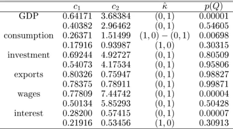
Table 4 shows the main results. We give the rst decision statistic c 1 which is inde- pendent of error scales, the second decision statistic c 2 which had to be re-scaled by division through the estimated standard deviation of the errors ^ , the discrete parame- ter estimate following from the decision statistics and from Table 1, using N = 100 for Germany, N = 150 for the United Kingdom, and interpolating between the two val- ues for Austria. In borderline cases, two possible estimates for the discrete parameter = ( i 1 ;i 2 ) are given. In the nal column we display the marginal signicance of Q , as stated above.

Notice that the main results dier from those of previous research based on classical methods. Most series show deterministic seasonality (0,1). In the Austrian data we nd seasonal unit roots (1,0) only in consumption and interest, in both cases only in the augmented test version. In the German data we nd seasonal unit roots also in the GDP and wages variables, also in the augmented version only. None of the British series is classied as having seasonal unit roots. British wages and interest are classied as (0,0).

The most conspicuous results are the deterministic nature of seasonality in investment,

which may be explained by the large share of the construction sector which is hit by

the climatic seasonal cycle, and the contradiction in the Austrian data between total

GDP and one of its main components, private consumption. The sum of a (1,0) and

a (0,1) variable is certainly (1,0) but the deterministic component in the added (0,1)

variable may be so strong that it disables statistical recognition of the unit roots in the

aggregate series.

TABLE 4. Estimates for discrete seasonal parameters (a) Austrian data

c1 ^c2

^

(

)

GDP 0

64171 3

68384 (0

1) 0

00001 0

40382 2

96462 (0

1) 0

54605 consumption 0

26371 1

51499 (1

0)

(0

1) 0

00698 0

17916 0

93987 (1

0) 0

30315 investment 0

69244 4

92727 (0

1) 0

80509 0

54073 4

17534 (0

1) 0

95806 exports 0

80326 0

75947 (0

1) 0

98827 0

78375 0

78911 (0

1) 0

99871 wages 0

77809 7

44742 (0

1) 0

00004 0

50134 5

85293 (0

1) 0

50428 interest 0

28200 0

57415 (0

1) 0

00007 0

21916 0

53456 (1

0) 0

30913 (b) German data

c1 ^c2

^

(

) GDP 0

50964 0

66334 (0

1) 0

00273

0

24993 0

53925 (1

0) 0

99217 consumption 0

64582 2

61653 (0

1) 0

00000 0

22901 1

36622 (1

0) 0

78246 investment 0

58391 2

47899 (0

1) 0

00742 0

33720 1

43830 (0

1) 0

99698 exports 0

76982 1

15883 (0

1) 0

07252 0

69788 1

01670 (0

1) 0

38479 wages 0

57569 2

22417 (0

1) 0

00000 0

15816 0

96554 (1

0) 0

79787 interest 0

19854 1

47223 (1

0) 0

00381 0

19931 1

13530 (1

0) 0

01730 (c) UK data

c1 ^c2

^

(

) GDP 0

55363 0

84969 (0

1) 0

00006

0

31064 0

49970 (0

1) 0

20413

consumption 0

65677 0

98788 (0

1) 0

00000

0

33142 0

54039 (0

1) 0

09775

investment 0

70979 1

46300 (0

1) 0

03056

0

35532 0

91398 (0

1) 0

98534

exports 0

60081 0

71460 (0

1) 0

31281

0

59381 0

74832 (0

1) 0

35700

wages 0

82293 0

47569 (0

0) 0

00408

0

51865 0

35802 (0

0) 0

49176

interest 0

77228 0

29415 (0

0) 0

68022

0

84159 0

32683 (0

0) 0

84557

5.2 Bivariate evidence

For the bivariate examples, pairs of real wages and real private consumption series for the three countries, i.e., Austria, Germany, and the United Kingdom were used.

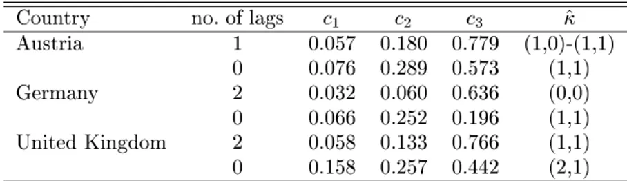
Seasonal patterns in wages may generate similar seasonal patterns in spending, hence seasonal cointegration seems to be the most interesting in these pairs. As in the last subsection, we report two sets of values for each case, one with enough conditioning lags to eliminate residual autocorrelation and one without conditioning. Noting that univariate analysis has found no evidence for seasonal unit roots in Austrian wages and both British series, the results in Table 5 appear surprising. In the United Kingdom, all seasonality is attributed to deterministic cycles and seasonal constants if no lag augmentation is used. After accommodating for serial correlation, a (1,1) model with seasonal cointegration is selected. Note that the (1,1) model has a seasonal unit root that is not found by the univariate selection procedure. In Austria, the results also support seasonal cointegration in the stochastic part whereas the evidence on the importance of seasonal dummies is not very pronounced. Depending on the interpolation between the b 3 bounds for N = 100 and N = 150, the c 3 value of 0.779 is ambiguous. In Germany, there is no seasonal cointegration but freely developing unit-root seasonality if lags are accounted for. The statistic c 3 would point to the presence of deterministic seasonality but this decision is overruled by the requirement of data admissibility.

TABLE 5. Estimates for discrete seasonal parameters in bivariate systems consisting of real wages and real private consumption.

Country no. of lags

^ Austria 1 0.057 0.180 0.779 (1,0)-(1,1)

0 0.076 0.289 0.573 (1,1)

Germany 2 0.032 0.060 0.636 (0,0)

0 0.066 0.252 0.196 (1,1) United Kingdom 2 0.058 0.133 0.766 (1,1) 0 0.158 0.257 0.442 (2,1)

In summary, the evidence is in conict with the univariate analysis. In univariate series,

a completely deterministic time series description is preferred in many variables. In

the bivariate series, the importance of seasonal unit roots in Austria and Germany

is underscored. This puzzle could be solved by the observation that the univariate

marginal processes are unit-root processes without seasonal constants indeed but can

be described satisfactorily over longer time intervals by simple seasonal constants plus a

suciently rich stationary cyclical structure. In other words, the changes in the seasonal

structure are too slow to justify the use of seasonal unit roots models for univariate

series, particularly as these unit roots cannot be used simultaneously with seasonal

dummies. A model that captures 90% of the seasonal variation, say, is preferred even if it is the `wrong' model. In contrast, bivariate models suggest the joint exploitation of the explanatory powers of seasonal dummies and of seasonal unit roots by restricted seasonal cointegration.

5.3 Sensitivity of the results

The empirical results presented up to here depend on the design of the MD analysis.

Slight changes in that design may have strong eects on the outcome. A decision maker may feel more comfortable if the main parameter estimates prove robust toward those changes. In classical hypothesis testing, this sensitivity is checked routinely by embed- ding the general model as dened on the primary parameter space in an even more general model by extending it to a larger primary parameter space

and by considering the decision problem of whether the data still select . For example, VAR models with Gaussian random errors are embedded in VAR models with non-Gaussian errors or in VAR models with rst-order autocorrelated Gaussian errors. In MD anal- ysis, this kind of sensitivity check is just one type of possible procedures and maybe not even the most amenable to its spirit. One may e.g. consider the following types of sensitivity checks:

1. Sensitivity with regard to adding or deleting a hypothesis 2. Sensitivity with regard to splitting or merging specied classes 3. Sensitivity with regard to the distributional window

4. Sensitivity with regard to opening or closing the structural part of the model window

5. Sensitivity with regard to the loss function

6. Sensitivity with regard to within-class priors or coordinate changes 7. Extending the class of decision rules with the aim of further gains in risk

For the metaphorical usage of the word `window' for the basic parametric most gen- eral model considered, cf. Poirier (1995). We adopt this metaphor in order to express our conviction that the validity of the most general model is not testable but rather represents a way of viewing the world of data, i.e. a `window'.

From this menu, only very few experiments can be conducted routinely although any

item may be of particular interest. Here, we conduct three sensitivity experiments.

Firstly, we consider the eects of cointegration at ! = 0 which was excluded from the basic simulation design and is often observed in macroeconomic time series. We note, however, that frequency-zero cointegration is not found by standard statistical tools in our bivariate examples.

The cointegration experiment is of type 4 according to the above list. In all classes of bivariate models, 50% of the generated processes are allowed to be cointegrated. A tech- nical problem is that, in the presence of cointegration at the frequency 0, hard rejection must be abandoned as a principle to generate multivariate uniform distributions. The chance to hit upon a non-explosive process of the form

4 X

= (1 ; 12 )

diag( 11 ; 0)(1 ; 12 ) S ( B ) X

1

+

2 A ( B ) X

1 +

3 2 X

2 + "

(16) is almost negligible for non-singular seasonal cointegration matrices

2 and

3 , i.e., in the case of no seasonal unit roots, if all matrices are still built upon their eigenvalues in the admissible ranges, i.e., (-2,0) for the frequency 0 and (0,2) for the seasonal frequencies. There are two conceivable solutions to this problem of additional cross- restrictions among the three frequencies. Firstly, one may rely on a uniform prior on the parameter 11 only and generate

2 and

3 by some prior distribution on the coecient space. Secondly, one may enforce the loading vectors and cointegrating vectors to be the same across frequencies and restrict all ve roots by a stability condition. In fact, this stability condition turned out to be simply

;

11 + 21 + 22 + 31 + 32

2

and a uniform distribution on this 5{variate area can be generated easily, so the latter solution was adopted. Here, 21 and 22 denote the eigenvalues of

2 and 31 and 32 denote the eigenvalues of

3 . This has the advantage that the very same design can be used for the seasonally cointegrated classes. However, whereas the classes (2,0) and (2,1) are unrestricted, a restriction is imposed on (1,0) and (1,1), as the seasonal cointegration vectors have to be the same. This circumstance may be responsible for the observed increase in expected risk.

Table 6 summarizes the results of this cointegration sensitivity check for N = 100. It

is obvious that the smaller non-zero seasonal root in the non-seasonal classes (2,0) and

(2,1) is less likely to be found in cointegrated processes. The MD procedure lowers the

corresponding decision bound in order to avoid larger losses for these misclassications

but pays with a strong increase of misclassications of the (1,1) processes with seasonal

cointegration and deterministic dummy cycles. However, the main results of the last