IHS Economics Series Working Paper 233
January 2009
A Nonparametric Test for Seasonal Unit Roots
Robert M. Kunst
Impressum Author(s):
Robert M. Kunst Title:
A Nonparametric Test for Seasonal Unit Roots ISSN: Unspecified
2009 Institut für Höhere Studien - Institute for Advanced Studies (IHS) Josefstädter Straße 39, A-1080 Wien
E-Mail: o ce@ihs.ac.atffi Web: ww w .ihs.ac. a t
All IHS Working Papers are available online: http://irihs. ihs. ac.at/view/ihs_series/
This paper is available for download without charge at:
https://irihs.ihs.ac.at/id/eprint/1891/
A Nonparametric Test for Seasonal Unit Roots
Robert M. Kunst
233
Reihe Ökonomie
Economics Series
233 Reihe Ökonomie Economics Series
A Nonparametric Test for Seasonal Unit Roots
Robert M. Kunst January 2009
Institut für Höhere Studien (IHS), Wien
Contact:
Robert M. Kunst
Department of Economics and Finance Institute for Advanced Studies Stumpergasse 56
1060 Vienna, Austria and
University of Vienna Department of Economics Brünner Straße 72 1210 Vienna, Austria
email: robert.kunst@univie.ac.at
Founded in 1963 by two prominent Austrians living in exile – the sociologist Paul F. Lazarsfeld and the economist Oskar Morgenstern – with the financial support from the Ford Foundation, the Austrian Federal Ministry of Education and the City of Vienna, the Institute for Advanced Studies (IHS) is the first institution for postgraduate education and research in economics and the social sciences in Austria.
The Economics Series presents research done at the Department of Economics and Finance and aims to share “work in progress” in a timely way before formal publication. As usual, authors bear full responsibility for the content of their contributions.
Das Institut für Höhere Studien (IHS) wurde im Jahr 1963 von zwei prominenten Exilösterreichern – dem Soziologen Paul F. Lazarsfeld und dem Ökonomen Oskar Morgenstern – mit Hilfe der Ford- Stiftung, des Österreichischen Bundesministeriums für Unterricht und der Stadt Wien gegründet und ist somit die erste nachuniversitäre Lehr- und Forschungsstätte für die Sozial- und Wirtschafts- wissenschaften in Österreich. Die Reihe Ökonomie bietet Einblick in die Forschungsarbeit der Abteilung für Ökonomie und Finanzwirtschaft und verfolgt das Ziel, abteilungsinterne Diskussionsbeiträge einer breiteren fachinternen Öffentlichkeit zugänglich zu machen. Die inhaltliche Verantwortung für die veröffentlichten Beiträge liegt bei den Autoren und Autorinnen.
Abstract
We consider a nonparametric test for the null of seasonal unit roots in quarterly time series that builds on the RUR (records unit root) test by Aparicio, Escribano, and Sipols. We find that the test concept is more promising than a formalization of visual aids such as plots by quarter. In order to cope with the sensitivity of the original RUR test to autocorrelation under its null of a unit root, we suggest an augmentation step by autoregression. We present some evidence on the size and power of our procedure and we illustrate it by applications to a commodity price and to an unemployment rate.
Keywords
Seasonality, nonparametric test, unit roots
JEL Classification
C12, C14, C22
Comments
The author wishes to thank Joerg Breitung, Philip Hans Franses, Helmut Luetkepohl, Bent Nielsen,
Contents
1 Introduction 1
2 The testing problem 2
3 Non-parametric tests based on quarter graphs 8
4 The RURS test 8
4.1 Records in ranges of seasonals ... 8 4.2 Lag augmentation ... 10 4.3 Forward and backward ... 15
5 Simulation evidence 16
5.1 Some remarks on distributions ... 16 5.2 Size and power ... 18
6 Extending the null and alternative 23 7 The monthly version of the RURS test 26 8 Empirical applications 28
9 Concluding remarks 31
References 32
1 Introduction
Since the possibly first contribution to the literature by Dickey et al. (1984), various authors have developed statistical test procedures for the discrimination of seasonal unit roots and purely determinis- tic seasonality in time series (for a survey on this literature and for the properties of the two model classes, see Ghysels and Osborn, 2001). Like the popular HEGY test by Hylleberg et al. (1990), most tests were created in a parametric autoregressive framework, where unit roots are the null and their non-existence is the alternative. The reverse tests by Caner (1998), Canova and Hansen (1995), and Tam and Reinsel (1997) can be viewed as semi-parametric, how- ever, with their null of a deterministic cycle and the background of an unobserved-components structure, as it is more typical of the litera- ture on seasonal adjustment rather than seasonal models. Hitherto, fully non-parametric tests on seasonal unit roots have not been in usage. It is the aim of this paper to consider this possibility.
For non-seasonal unit roots, So and Shin (2001) and Aparicio et al. (2006, AES) developed genuine non-parametric testing procedures.
Such tests are most commonly applied in the presence of non-linear features (for example, see Choi and Moh, 2007). The tests exploit properties of time series that are not linked to moments but are nev- ertheless characteristic of integrated versus stationary processes, such as sign changes, zero crossings, or the occurrence of new extrema. By construction, sign and extrema features are robust or even entirely invariant to nonlinear transformations of variables and to occasional but rare outliers and level shifts. For this reason, nonparametric tests can be helpful if nonlinear transformations of linear time-series models are plausible data-generating mechanisms and also if the error process indicates strong deviations from the normal distribution. The ob- vious drawback is that nonparametric tests lack power as compared with parametric tests if the investigated time series indeed conform to standard assumptions.
A less obvious drawback for nonparametric testing for unit roots is that the ideas typically rely on properties of pure random walks.
The generalization of random walks to integrated processes imposes
problems, as the serial correlation of increments invalidates the un-
derlying statistical results. Thus, while the frequency of new extrema
in the logarithm of a random walk with positive values is the same as
in an untransformed random walk, it is severely affected if the first
difference of the observed variable follows a stable autoregression. A
suggestion is then to filter the original data in order to remove auto-
correlation. To that aim, one may consider frequency-domain filters
or conditioning on lags, as in the ‘augmentation’ of the Dickey-Fuller test. In this paper, we follow the latter route and condition on some lags determined by an auxiliary regression.
Intuitively, it may appear simple to construct a non-parametric test for seasonal unit roots on the basis of by-season time-series plots, as they have been suggested by Franses (1994, 1996) and are being implemented into major software programs. Usually, occurring inter- sections among seasons—in most cases, quarters—are interpreted as evidence on changes in the seasonal pattern. However, this informal test is unlikely to be very rigorous, as variables with a weak seasonal pattern will intersect even more frequently. For this reason, we con- sider a test that parallels the known test procedure by Aparicio et al. (2006) in a context of possible seasonal unit roots.
This paper is organized as follows. Section 2 sets up the testing problem of interest and defines the maintained model. Section 3 con- siders the simple testing idea of monitoring seasonal crossings that was outlined above. Section 4 introduces our RURS (records unit root seasonal) test, a seasonal variant of the AES procedure. Sec- tion 5 presents some Monte Carlo simulations for assessing the size and power properties of the test. Section 6 considers the issue of ro- bustness of the test to extended maintained hypotheses. Section 7 addresses the RURS test at the monthly frequency. Section 8 reports the application of the test to economics examples. Section 9 concludes.
2 The testing problem
We wish to consider time-series variables that are generated by auto- regressions—possibly with unit roots—that are superseded with de- terministic cycles and possibly a linear trend function. That is, x
tfor t = 1, 2, . . . , n is assumed to follow
x
t= x
∗t+
4
X
j=1
γ
j∗D
jt+ c
∗t, (1) with the purely stochastic autoregressive process (x
∗t), where D
jtde- notes the usual seasonal dummy variables. For t = 0, . . . , − 3, x
thas some given non-stochastic starting values. At first, we constrain the autoregressive lag order to be less equal four, such that the AR(4) model
x
∗t=
4
X
j=1
a
∗jx
∗t−j+ z
twith white-noise z
tand starting values x
∗t= 0 for t ≤ 0 is correctly
specified. The process (z
t) is Gaussian white noise in the most re-
stricted specification. More general conditions will be introduced be- low.
In the spirit of testing for seasonal unit roots, the focus is not on the properties of the deterministic cycle. In other words, a model with γ
∗j= γ
∗is seen as a special case of a model with ‘deterministic seasonality’ if the purely stochastic part (x
∗t) does not have seasonal unit roots.
The presentation here is tuned to the case of quarterly time series with the periodicity of four. The generalization to the monthly case or to any other periodicity is straight forward. However, these cases demand for some complexity in notation and introduce some subtle problems that will be addressed in Section 7.
In the representation (1), the interpretation of the constant 4
−1P
4j=1
γ
j∗is independent of the unit-root event H
0: P
4j=1
a
∗j= 1. It is an av- erage mean of the process (x
t) following linear de-trending by c
∗t.
Potential drift under H
0is handled by the trend coefficient c
∗. The process (x
t) has an interesting alternative parameterization that is sometimes called the ‘spectral’ or ‘cycles’ representation:
∆
4x
t= µ + a
1x
(1)t−1+ ct + a
2x
(2)t−1− γ
2( − 1)
t+a
3∆
2x
t−2+ a
4∆
2x
t−1− (a
3+ a
4)
2(γ
3s
t−2+ γ
4s
t−1) + z
t, (2) with the notation
x
(1)t= x
t+ x
t−1+ x
t−2+ x
t−3, x
(2)t= x
t− x
t−1+ x
t−2− x
t−3,
∆
mx
t= x
t− x
t−m, m = 2, 4, s
t= sin πt/2.
It is not difficult to see that equations (1) and (2) describe the same model class. The equivalence of the customary parameteriza- tion (a
∗1, . . . , a
∗4) of a fourth-order autoregression and (a
1, . . . , a
4) is the basis for the traditional HEGY test. The correspondence between the drift term c
∗and the intercept µ is rather trivial, and the transi- tion between (γ
∗j, j = 1, . . . , 4) and (γ
j, j = 1, . . . , 4) follows from the details in Smith and Taylor (1999). Note that the parameter di- mension of representation (2) exactly corresponds to model (1), with 4
−1µ denoting the drift under H
0and the added linear trend only activated under H
0C.
The handling of the deterministic terms serves as a ‘bridle’ that
contains implausible expansion at the seasonal frequencies. Similar
bridle devices are common in multivariate models (see Johansen,
1995) to contain trending behavior at the zero frequency in the case of unit roots. For a similar purpose, Dickey and Fuller (1979) suggested F–tests for the joint hypothesis of a unit root and zero con- stant. Note, however, that model (1) does not restrict the trend at the zero frequency. The effects of constants at the trend frequency and of deterministic cycles at the seasonal frequencies are different.
A constant together with a unit root at +1 generates a linear trend in x
t, which is not an implausible specification for economic data. A trigonometric cycle together with a unit root at − 1 or at ± i gener- ates linear expansion of seasonal cycles, which may be regarded as implausible. See Franses and Kunst (1999) for a similar argument in multivariate seasonal models.
The spectral representation (2) is important for our purposes, as it directly motivates testing for the a
jcoefficients in order to check events of seasonal unit roots. It is obvious that (x
t) ‘has a unit root at +1’ if and only if a
1= 0, and it ‘has a unit root at − 1’ iff a
2= 0.
The unit roots at ± i can only occur jointly, and they do so if and only if (a
3, a
4) = (0, 0). The spectral representation also serves as a device for generating alternatives in the reported simulations, where γ
jrather than γ
∗jvalues will be set.
The range of admissible (z
t) terms is constrained by the so-called Berman condition, which suffices for the derivation of extremal prop- erties. Our first assumption concerns the parametric space that we wish to investigate as the maintained hypothesis, the second assump- tion concerns the properties of the errors process. Throughout, we use B to denote the lag operator.
Assumption 1 There is a representation
(1 − B )
m1(1 + B)
m2(1 + B
2)
m3x
t= ˜ x
t,
such that (˜ x
t) is stationary, where m
j∈ { 0, 1 } for j = 1, . . . , 3. The representation is unique if m
jis defined as the minimum value that achieves stationarity in x ˜
t.
The word ‘stationary’ is meant to include the possibility of transi- tory deviations from strict stationarity due to starting values and to allow for an added four-periodic deterministic cycle and a linear time trend. Assumption 1 is roughly equivalent to the following one:
Assumption 1 (
′) The polynomial Φ(z) defined by
Φ(z) = 1 − z
4− a
1(z + z
2+ z
3+ z
4) − a
2(z − z
2+ z
3− z
4)
− a
3(z
2− z
4) − a
4(z − z
3)
has no roots outside the set
{ z ∈ C : | z | > 1 } ∪ {± 1, ± i } , and all roots within the latter set have multiplicity one.
Note that Φ(z) can be even uniquely defined if the generating law is an AR process with p > 4, for example by splitting off the roots with largest modulus. This would take care of the case of more general stationary but serially correlated z
t, for example stationary ARMA.
These assumptions exclude explosive roots, multiple unit roots, and unit roots at bizarre frequencies. We use the term ‘bizarre’ to describe unit roots at values different from the main spectral fre- quencies. For example, the second-order autoregressive model y
t= φ
1y
t−1+ φ
2y
t−2+ ε
thas the well known triangular stability area for its coefficients. One of the boundaries of the triangle, the open hor- izontal line segment { (φ
1, − 1), − 2 < φ
1< 2 } , describes models with bizarre frequencies, excepting the point (0, − 1). Such unit roots are rare in empirical applications.
Assumption 1 is satisfied for small negative a
1and small positive a
2and a
3. The coefficient a
4interacts with a
3in a complicated way.
For a
3> 0, the model will remain stable for a relatively wide range of a
4values.
Assumption 2 If at least one of the values m
jis 0, the stationary process (˜ x
t) considered in Assumption 1 fulfills a Berman condition. A stationary process with autocorrelations c
kis said to fulfill a Berman condition if c
klog k → 0 as k → ∞ .
This condition is adopted by AES to define the alternative model for their unit-root test. For seasonal tests, it may make sense to demand this property not only from processes under the ‘total’ alter- native of stationarity but also from transformed processes that are in the alternative of some hypothesis but in the null of others. For ex- ample, (a
1, a
2, a
3, a
4) = (0, 1/2, 1/2, 1/2) defines a process with a unit root at +1 but no other unit root, in the symbols of Assumption 1 (m
1, m
2, m
3) = (1, 0, 0). Its first differences ˜ x
t= ∆x
tare stationary and should have the Berman property.
Obviously, the usage of the liberal Berman condition to define the properties of the classes of interest entails that the tests are not designed to discriminate unit roots in the traditional I(1) sense from fractional alternatives. The Berman condition holds for stationary ARMA as well as for I(d) with d < 0.5.
Technically, the Berman condition ensures the asymptotic valid-
ity of extremal distributions under the I(0) hypothesis if additionally
normality is assumed. For non-normal distributions, general mixing conditions are required. A sufficient mixing condition is the D(u
n) condition by Leadbetter and Rootz´ en (1988).
Depending on appropriate assumptions on the error process (z
t) that should cover stable autoregressions as well as invertible moving- average processes, the model class defined in (1) is pretty general.
It comprises the seasonal random walk (SRW) for (a
1, a
2, a
3, a
4) = (0, 0, 0, 0) with or without drift, and it also covers I(1) processes with added deterministic seasonal cycles. It also permits the occurrence of, for example, a seasonal unit root at − 1 but not at ± i together with a quarterly deterministic seasonal cycle that can be expressed as the sum of s
tterms. The bridle excludes processes with expanding deterministic seasonal variation, and we also do not wish to consider superlinear trends.
It would be convenient if processes with seasonal unit roots, in generalization of the usual I(1) hypothesis, could be used as null hypotheses. Unfortunately, even in the non-seasonal model little is known about the properties of basic test statistics and their asymp- totic distributions for general I(1) processes. The tests considered by AES and by Burridge and Guerre (1996) rely on the assumption of pure random walks, i.e. cumulative sums of i.i.d. random variables, under their null. This special case is much too restrictive for typical econometric applications, where increments show considerable pos- itive serial correlation. We will introduce a correction that serves to at least approximately retain the distributional properties for the random-walk null in the correlated case. Robustness in this direction will be explored with the help of simulations.
Our test mainly builds on the ‘range unit-root’ (RUR) test that was suggested by AES. The test bears little relation to the range of the variables, so we prefer to read its acronym as ‘records unit-root’.
Its idea is to count the ‘records’, i.e. new extrema in the time-series sequence. Consider the maximum x
j,jand the minimum x
1,jof j successive time-series observations x
k, k = 1, . . . , j. If a new minimum or maximum is encountered, as j is increased, this is called a record.
In the following, the number of such records that occur until time point j will be denoted by R(j), or, to mark the time-series label, as R
(x)(j).
As j increases, the record count R(j) will also increase. For random walks, it can be shown that R(n) = O(n
1/2) as n → ∞ . For i.i.d.
sequences, the slower rate R(n) = O(log n) can be established. This
proposition can be generalized to many stationary processes. AES
give as the weakest possible condition the D(u
n) mixing property that
was mentioned above. At the other end of the scale, for drifting I(1)
processes, the faster rate R(n) = O(n) holds on quite general grounds.
For a
1= 0 and a
2= a
3= a
4= 1/2, Φ(z) = 1 − z and (x
t) becomes a random walk, assuming white noise (z
t). For the random walk with i.i.d. increments, we have the following theorem by AES:
Theorem 1 If (x
t) is a random walk with i.i.d. increments, and if the probability law of these increments fulfills some regularity condi- tions (p.d.f. is bounded and continuous, second moments are finite, expectation is zero), the statistic J
0(n)= n
−1/2R
(x)(n) converges to a well-defined probability law as n → ∞ .
AES provide a characterization of the asymptotic distribution and they show that it is well approximated in samples of moderate size.
Roughly, the unimodal p.d.f. peaks at the value 2 and its left-tail crit- ical points are around the value of 1. We will refer to this distribution as the ‘AES distribution’ in the following.
When there are no unit roots, i.e. if all roots of Φ(z) are confined to the set { z ∈ C : | z | > 1 } , AES prove another result:
Theorem 2 If (x
t) is a stationary Berman process, the statistic J
0(n)converges to 0 in probability as n → ∞ .
This theorem establishes the consistency of the RUR test that relies on the statistic J
0with regard to its left tail against a stationary alternative. In fact, the test is also consistent in its right tail against a drifting alternative. However, this property will not be in focus in this paper. We further note that it is obvious that the procedure may have little power in the presence of sub-linear trends
Rather than in testing H
0: (a
1, . . . , a
4) = (0, 1/2, 1/2, 1/2), we will be concerned with testing the more general hypotheses
H
0+: a
1= 0, H
0−: a
2= 0,
H
0i: a
3= a
4= 0, (3)
which correspond to unit roots at +1 (m
1= 1), at − 1 (m
2= 1) and at ± i (m
3= 1), respectively. In the following, we will address the hypotheses by these roots of Φ(z) and also alternatively by the corresponding angular frequencies at ω = 0, ω = π, and ω = π/2.
Before we will fully introduce an adequate test for the hypotheses
H
0+, H
0−, H
0ithat parallels the AES idea, we consider a suggestion
from the literature in the following section.
3 Non-parametric tests based on quar- ter graphs
Several monographs on seasonality recommend plots of time series by quarters (see, e.g., Franses, 1994, 1996, or Ghysels and Osborn, 2001). Apparently, the frequency of rank changes among quarters is viewed as an indicator that eases the classification of the time series with respect to the main seasonal models. One may presume that seasonal unit-root processes entail infrequent rank changes, while de- terministic seasonality might imply few changes when it is pronounced, and very frequent changes when it is weak.
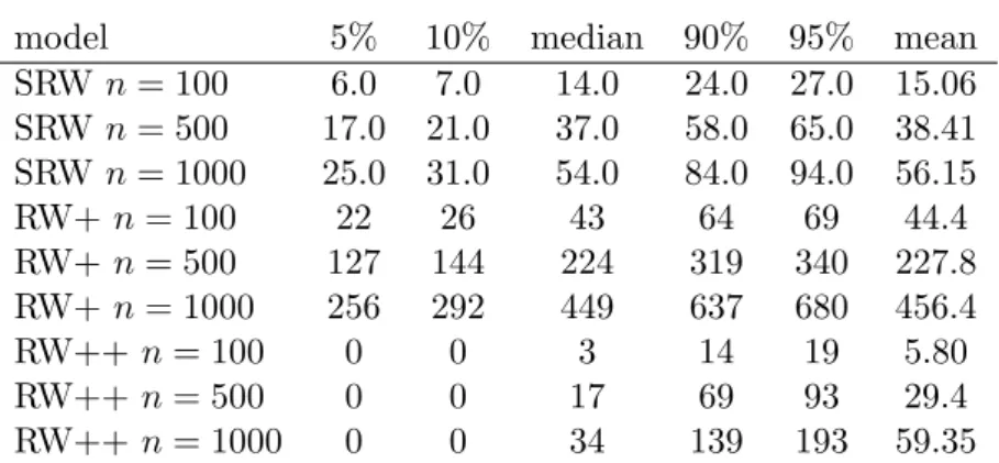
Table 1 displays the rank changes counted in a small Monte Carlo experiment. First, seasonal random walks (SRW) were generated from zero starting values, and changes in ranking were counted. Then, random walks were generated with an added seasonal pattern that was fixed within one trajectory and drawn from four further normal random numbers. In ‘RW+’, the same variance was used for the increments and the seasonal pattern. In ‘RW++’, the variance of the seasonal pattern was 100 times the variance of the increments, which is not unusual in some empirical examples. 10,000 replications were used to determine quantiles of the empirical distribution and the mean.
The results conform to expectations and indicate that counting rank changes cannot be a very reliable test. For the weak seasonal pattern in RW+, the average frequency of rank changes is close to n/2, while for the strong seasonal pattern in RW++, the distribution is very asymmetric and its mean is of a magnitude that is comparable to the case of a seasonal random walk.
4 The RURS test
4.1 Records in ranges of seasonals
The results by AES on the RUR test suggest using the record count as a tool for discriminating stationary and integrated variables. The fact that the limit distribution for the random walk has an established although not simple form suggests using the random walk as a null hy- pothesis and rejecting for too small values—which are representative of the stationary alternative—as well as for too large values—which may represent processes with a deterministic drift. However, econo- mists are rarely interested in testing for the existence of a drift and prefer to test for unit roots that reflect permanent effects of shocks.
Therefore, we will use the tests in their one-sided versions and ex-
Table 1: Changes of ranking in simulated trajectories.
model 5% 10% median 90% 95% mean
SRW n = 100 6.0 7.0 14.0 24.0 27.0 15.06 SRW n = 500 17.0 21.0 37.0 58.0 65.0 38.41 SRW n = 1000 25.0 31.0 54.0 84.0 94.0 56.15
RW+ n = 100 22 26 43 64 69 44.4
RW+ n = 500 127 144 224 319 340 227.8
RW+ n = 1000 256 292 449 637 680 456.4
RW++ n = 100 0 0 3 14 19 5.80
RW++ n = 500 0 0 17 69 93 29.4
RW++ n = 1000 0 0 34 139 193 59.35
Note: SRW denotes that the generating model is a seasonal random walk. RW+ denotes a random walk with an added deterministic cycle that is drawn with the same variance as the increments. RW++ denotes that the seasonal standard error is ten times the standard deviation of the increments. Columns headed by percentages collect empirical quantiles.
tract potential deterministic time trends, in analogy to So and Shin (2001).
If x
tis an SRW x
t= x
t−4+ ε
trather than a random walk, the autoregressive operator contains four unit roots at ± 1, ± i. Within the model class defined by (2) and Assumptions 1 and 2, one may be interested in considering the three null hypotheses H
0+, H
0−, H
0i. These hypotheses can be addressed after transforming the original SRW in order to eliminate all other unit roots that are not under immediate consideration.
First, the four-quarter moving average
x
(1)t= x
t+ x
t−1+ x
t−2+ x
t−3is a pure random walk if x
tis a SRW. Parametric unit-root tests or the RUR test can then be applied to x
(1)t. This statistic is denoted by J
1here and is designed to test for H
0+. The properties of the RUR statistic under H
0+depend on the validity of the other unit-root hy- potheses H
0−and H
0i. For example, if x
tis a random walk, it should be classified under H
0+but the increments of x
(1)tare autocorrelated and follow a third-order non-invertible moving-average process. The limiting distribution of the RUR statistic is not known for this case.
For technical reasons, we convene the notation x
[1]t= x
(1)t. Second, the four-quarter alternating moving average
x
(2)t= x
t− x
t−1+ x
t−2− x
t−3is a ‘mirror’ random walk x
(2)t= − x
(2)t−1+ ε
tif (x
t) is a SRW. The adjusted process x
[2]t= ( − 1)
tx
(2)tis a regular random walk and can be subjected to the RUR test. The corresponding RUR statistic is denoted by J
2here and is designed to test for H
0−. The process (x
[2]t) contains a unit root at +1 even if (x
t) is not a SRW, as long as (x
t) conforms to H
0−. Then, however, again the distribution of the RUR statistic will change.
Third, the second-order difference
∆
2x
t= x
t− x
t−2follows the simple law ∆
2x
t= − ∆
2x
t−2+ε
tif x
treally is a SRW. Two separate random walks x
[3]tand x
[4]tcan be constructed by sampling only every other observation and multiplying every other observation of either process by − 1. Again, these two random walks can be sub- jected to RUR tests, and the RUR statistics will follow the AES dis- tribution for either process. These statistics are denoted by J
3and J
4and they are designed to test for H
0i. However, they will deviate from the AES distribution if the original x
tcontains a unit root at ± i but is not a SRW. Note that the sample size is halved for this test. In the following, the collection of the four tests based on J
j, j = 1, . . . , 4 for the unit-root hypotheses H
0+, H
0−, H
0iwill be called the RURS test, for ‘records unit-root seasonal’.
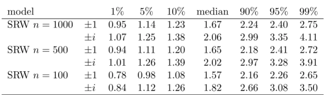
Table 2 gives simulated quantiles for all four statistics if the gener- ating process is a SRW. The quantiles correspond well to those given by AES. Statistics J
1and J
2as well as J
3and J
4have almost iden- tical empirical distributions even in fairly small samples, and their simulation results are given only once.
4.2 Lag augmentation
We first summarize the fundamental asymptotic properties in a theo- rem.
Theorem 3 Under assumptions 1 and 2, the following two properties hold:
(a) If (x
t) is a seasonal random walk with regular i.i.d. increments and thus is an element of H
0+∩ H
0−∩ H
0i, the distribution of all statistics J
j, j = 1, . . . , 4 converges to the law indicated by AES;
(b) If (x
t) is in the alternative of any of the three hypotheses H
0+,
H
0−, H
0i, the corresponding test statistic J
jwill converge to 0
as n → ∞ .
Table 2: RURS test. Simulated quantiles from 10,000 replications.
model 1% 5% 10% median 90% 95% 99%
SRW n = 1000 ± 1 0.95 1.14 1.23 1.67 2.24 2.40 2.75
± i 1.07 1.25 1.38 2.06 2.99 3.35 4.11 SRW n = 500 ± 1 0.94 1.11 1.20 1.65 2.18 2.41 2.72
± i 1.01 1.26 1.39 2.02 2.97 3.28 3.91 SRW n = 100 ± 1 0.78 0.98 1.08 1.57 2.16 2.26 2.65
± i 0.84 1.12 1.26 1.82 2.66 3.08 3.50
Note: SRW denotes that the generating model is a seasonal random walk. Rows ±1 correspond to theJ1andJ2statistic with identical performance, while rows±icorrespond to theJ3andJ4statistics.The proof of this theorem is obvious from AES. For an SRW, all transforms (x
[j]t), j = 1, . . . , 4 are random walks, and under the alter- natives the Berman conditions will hold even for dynamic transforms of the processes that obey Berman’s conditions because of assumption 2. Note that the theorem is silent, for example, on the properties of J
j, j 6 = 2 on H
0+∩ H
0−c, and even on processes in H
0+∩ H
0−∩ H
0ithat are not pure SRW.
Unfortunately, even for the standard RUR test by AES very little can be said about general I(1) processes that serve as the null hy- pothesis. While the limiting distribution is valid for nonlinear trans- formations of random walks, it is invalidated by deviations from the i.i.d. assumption on increments. A simple simulation shows that the AES distribution becomes indeed completely distorted if increments are serially correlated.
Thus, the test is not similar unless the null hypothesis is restricted to the very special case of a SRW with i.i.d. increments. In order to achieve approximate similarity for the more general null hypotheses of interest, we suggest a parametric autoregressive correction in the spirit of the ADF test. To this aim, we first consider the four variables x
[j]t, j = 1, . . . , 4
x
[1]t= x
(1)t, t = 1, . . . , n, x
[2]t= ( − 1)
tx
(2)t, t = 1, . . . , n, x
[3]t= ( − 1)
t∆
2x
2t, t = 1, . . . , n/2,
x
[4]t= ( − 1)
t∆
2x
2t−1, t = 1, . . . , n/2. (4)
Ideally, all of these variables follow random walks and their first dif- ferences are i.i.d. white noise. If there is low-order autoregressive autocorrelation, then the residuals
u
j,t= ∆x
[j]t− µ −
p
X
k=1
φ
k∆x
[j]t−kwill be white noise. In practice, these true residuals will be replaced by least-squares regression residuals ˆ u, although alternative estimation techniques may deserve consideration. In a final step, the residuals ˆ u
j,tcan be accumulated again, and the cumulative sums,
˜
x
[j]t= x
[j]p+
t
X
r=p+1
ˆ
u
j,r, (5)
say, are then subjected to the original RUR test.
There is a danger that the ‘augmenting’ correction does more harm than good. If the analyzed process is really an ARIMA(p,1,0) in the familiar Box-Jenkins notation, consistent information criteria will find the true p, and at least for large n the procedure will yield a pure ran- dom walk. Unfortunately, if the original series does not have unit roots at all different frequencies, the process at hand will have a non- invertible ARIMA(p,1,q) structure and fitting autoregressions will re- sult in large p and will nonetheless be unable to correct completely.
This again will hamper the power of the test in case the alternative model at the investigated frequency holds.
Therefore, we tend to take care that p remains reasonably low.
Parsimonious criteria such as the consistent BIC rather than liberal ones like AIC are an obvious choice. Also, we restrict the maximum order in the BIC search by a slow function of the sample size. Some experimentation with different upper bounds shows that, for moderate n, a bound of n
1/4appears to be a good choice. In particular, n
1/4yields better power properties than customary bounds proportional to n
1/3at values distant from the null, where the augmentation tends to over-correct, at little expense for the size properties.
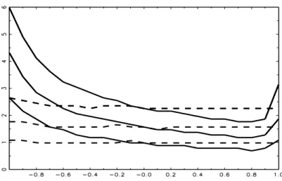
Essentially, we find indications for good performance but we also find critical issues in extensive simulations that we can only partially report. For example, Figure 1 demonstrates that the procedure works well with respect to the null distribution around the mode. The de- sign for this simulation is a SRW with first-order autoregressive er- rors, and the evaluated test statistic is the one for the root at − 1.
The picture shows that the 10%, 50%, and 90% quantiles of the null
distribution are unaffected by the autoregressive coefficient, even for
non-stationary cases such as +1 and − 1.
Figure 1:
10%, 50%, and 90% quantiles for the uncorrected (solid) and for the augmentation-corrected (dashed) RURS statistic J2(n) if it is calculated from trajecto- ries of length n = 100 from the data-generation process ∆4xt = φ∆4xt−1+εt and φ is varied over the interval [−1,1]. φvalues on the abscissa.The situation is comparable in the presence of moving-average er- rors, as Figure 2 demonstrates. The generation process is defined as x
t= x
t−4+ ε
t+ θε
t−1, and θ varies over the interval [ − 1, 1]. Because the seasonal differences are a first-order moving average process, sta- tistics J
3and J
4are unaffected. For J
1, θ = − 1 actually defines a process without a unit root at +1, as the unit roots in the autoregres- sive and the moving-average operator cancel. Similarly, for J
2, θ = 1 defines an element of the alternative.
Both figures show that the uncorrected statistic J
2(100)is severely distorted. For the augmentation-corrected statistic, shown quantiles remain flat over all negative θ values and react for larger positive values. Whereas the resilience in the negative area is to be appreciated, the reduced sensitivity in the positive area points to a loss in power relative to the uncorrected original statistic. For example, the 1%
quantile falls from the value θ = 0 to θ = 1 by a sizeable amount of 0.5 in the uncorrected case, while this difference reduces to 0.4 in the corrected case.
Similar simulations were conducted for the statistics J
1, J
3, J
4, and the performance was comparable to the H
0−case reported in Figures 1 and 2.
We note that the inclusion of a constant in the set of conditioning
regressors, even if BIC suggests no augmentation, results in eliminat-
ing a possible drift as well as all seasonal deterministic terms. The
latter property is grounded in the transformations that are used in
Figure 2:
10%, 50%, and 90% quantiles for the uncorrected (solid) and for the augmentation-corrected (dashed) RURS statistic J2(n) if it is calculated from trajecto- ries of lengthn= 100 from the data-generation process ∆4xt=εt+θεt−1 andθis varied over the interval [−1,1]. θ values on the abscissa.constructing x
[j]t, j = 1, . . . , 4, which together with the sign-change and sample-split operations eliminate all cycles of length 2 and 4 ob- servations. We also note that the constructed processes x
[j]tdo not necessarily have zero mean, as the cumulation is started from actual starting values. It is obvious, however, that the counting of records is unaffected by universal level shifts. It is exactly these robustness properties that have motivated the usage of non-parametric tests like RUR in the presence of potential features that are so typical for many economic time series, such as local aberrations, outliers, and local level shifts.
A critical issue that may deserve further study, however, is the occurrence of outliers and the reaction of the augmenting step. It is known from the time-series literature that least-squares estimation is robust to innovations outliers but is critically affected by additive outliers (see also Kleiner et al., 1976). Hence, whereas the correction works well for non-normal distributions of innovations, it is easy to construct examples where it fails for added outliers. If added outliers are a known feature of a data set, it may be advisable to replace the least-squares estimator by a robust procedure.
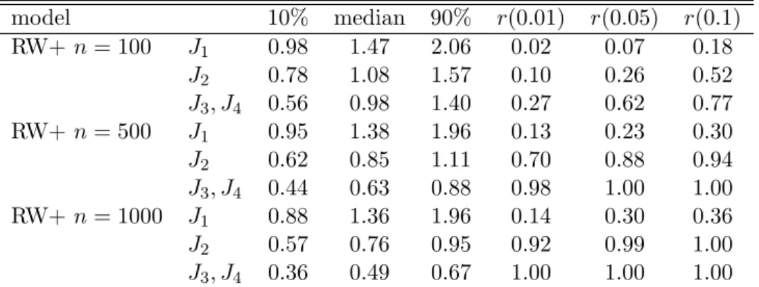
Table 3 reports a casual power simulation that can be compared to
the results on the graphical test of Section 3. The RW+ design of Ta-
ble 1 is used at the sample sizes n = 100, 500, 1000. For this process, J
1should not reject, while J
j, j = 2, . . . , 4 should reject the non-existing
seasonal unit roots. This case is particularly interesting, as processes
(x
[j]t) by construction have non-invertible moving-average parts that are a handicap for autoregressive augmentation. Augmentations are sizeable, double-digit lag orders are the rule for n = 1000. Table 3 demonstrates that power properties at the seasonal roots are accept- able but that the BIC augmentation is slightly too weak to preserve the size for the test based on J
1. Experiments with stronger augmen- tation, however, indicate a severe loss of power for the seasonal tests for H
0−and H
0iand tend to discourage more liberal augmentation.
Table 3: Power of RURS test. Simulated quantiles from 10,000 replications and rejection frequencies.
model 10% median 90% r(0.01) r(0.05) r(0.1)
RW+ n = 100 J
10.98 1.47 2.06 0.02 0.07 0.18
J
20.78 1.08 1.57 0.10 0.26 0.52
J
3, J
40.56 0.98 1.40 0.27 0.62 0.77
RW+ n = 500 J
10.95 1.38 1.96 0.13 0.23 0.30
J
20.62 0.85 1.11 0.70 0.88 0.94
J
3, J
40.44 0.63 0.88 0.98 1.00 1.00
RW+ n = 1000 J
10.88 1.36 1.96 0.14 0.30 0.36
J
20.57 0.76 0.95 0.92 0.99 1.00
J
3, J
40.36 0.49 0.67 1.00 1.00 1.00
Note: RW+ denotes that the generating model is a random walk with added seasonal constants drawn from a N(0,1) distribution. Row J3, J4 corresponds to both theJ3 and J4statistic with almost identical performance. r(p) denotes rejection frequency when the RURS test is used at a significance level ofp.A more systematic study of size and power properties will be the topic of Section 5.
4.3 Forward and backward
In order to increase the power of their RUR statistic, AES suggest to run the test in both directions, that is to count records from t = 1 to t = n and also from t = n to t = 1, and then to average the two thus obtained test statistics. Indeed, the laws of motion of random walks as well as of stationary processes have known time reversibility properties, and the additional information can serve in improving test performance.
In line with the AES notation, we denote the thus obtained RURS-
fb (‘fb’ for ‘forward-backward’) statistics by J
∗j, j = 1, . . . , 4. We also
keep the convention by AES to define these statistics via J
∗j= 2
−1/2(J
j+ J
j′),
rather than by the arithmetic mean, where J
j′denotes the reverse version of J
j. Note that, if J
jand J
j′were independent, this definition would increase scales by a factor √
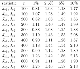
2. Table 4 provides a collection of corresponding significance points.
Table 4: Empirical null distribution of the RURS-fb test statistic.
statistic n 1% 2.5% 5% 10%
J
∗1, J
∗2100 0.81 1.03 1.18 1.77 J
∗3, J
∗4100 1.07 1.28 1.49 1.92 J
∗1, J
∗2200 0.82 1.08 1.23 1.85 J
∗3, J
∗4200 1.11 1.40 1.47 1.99 J
∗1, J
∗2300 0.88 1.08 1.25 1.88 J
∗3, J
∗4300 1.19 1.43 1.55 2.08 J
∗1, J
∗2400 0.90 1.11 1.26 1.87 J
∗3, J
∗4400 1.18 1.44 1.54 2.10 J
∗1, J
∗2500 0.90 1.12 1.28 1.89 J
∗3, J
∗4500 1.23 1.42 1.56 2.15 J
∗1, J
∗2600 0.91 1.11 1.26 1.90 J
∗3, J
∗4600 1.25 1.46 1.58 2.13
Note: Simulated quantiles from 20,000 replications of seasonal random walks. nis sample size, columns denoted ‘p%’ denote quantiles of the empirical distribution.
In the remainder of the paper, the focus will be on this RURS-fb version.
5 Simulation evidence
5.1 Some remarks on distributions
In our simulations, we generally found that the empirical distribution does not coincide with the one reported by AES, neither at the fre- quency zero nor at ± i. In this subsection, we attempt to explain the discrepancies.
Firstly, the limit distribution derived by AES builds on properties of Brownian motion. In a rough interpretation, the limit law describes the probability of range expansions over a Brownian motion process.
This is not an accurate statement, as the concept of range expansion
0.2.4.6.81
0 2 4 6
tied−down Random Walk Random Walk
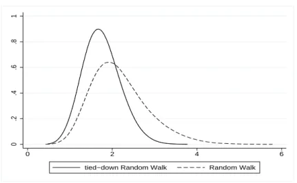
Figure 3:
Empirical densities of the RUR statistic for 500 observations. Random walk and drift-adjusted random walk, 20000 replications, Epanechnikov kernel estimation.makes little sense for a continuous-time process but it comes close to the asymptotic behavior.
By contrast, the intermediate augmenting step eliminates all trends and drifts in any random-walk trajectory. Therefore, the limit law does not build on a Brownian motion but rather on a Brownian bridge.
Figure 3 compares the empirical distributions of the RUR statistic for random walks and for adjusted random walks. The adjustment will re- duce findings of new extrema for many cases. Roughly, random walks sometimes expand near-monotonically and then extrema are becoming much sparser after correction. Conversely, sometimes random walks tend to generate pseudo-cycles, in which case extrema may become even more frequent after adjustment. The first effect appears to be stronger.
Second, the distribution of the RURS statistics does not even cor- respond to the Brownian bridge version due to the effects of the aug- menting step.
A technical detail concerns the handling of the first few observa- tions x
[j]tfor t < p (see equation (5)). We experimented with keeping them within the extrema search and also with excluding them. On the whole, we recommend running the search for records after exclud- ing the starting observations, as these may mask other extrema in the presence of outliers.
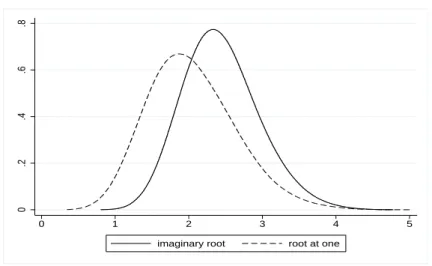
Figure 4 conveys an impression of the empirical distributions for
the actual statistics that are used in the RURS test.
0.2.4.6.8
0 1 2 3 4 5
imaginary root root at one
Figure 4:
Empirical densities of the RURS statistic for 500 observations. Seasonal random walk, 20000 replications, Epanechnikov kernel estimation.5.2 Size and power
In our size simulations, we compare the properties of the HEGY test and of the RURS test in its forward-backward (fb) variant. Quarterly seasonal random walks are generated in 10,000 replications for the (extended) sample sizes n = 100 to n = 600. These numbers corre- spond to 25 to 150 years and they are designed to cover the typical applications of economic relevance.
In detail, HEGY statistics are calculated from regressions
∆
4x
t= µ +
4
X
j=1
γ
jD
∗tj+ a
1x
(1)t−1+ a
2x
(2)t−1+ a
3∆
2x
t−2+ a
4∆
2x
t−1+
p
X
j=1
ζ
j∆
4x
t−j+ u
t, (6)
where the t–statistics on a
1and a
2and the F–statistics on (a
3, a
4) constitute the HEGY statistics on the three frequencies of concern.
The lag order p is found by minimizing BIC in the Schwarz variant, just as described before for the RURS test.
Characteristics of the empirical distributions are obtained from these null simulations. Because of the BIC–guided lag orders, they differ slightly from the small-sample quantiles reported in the litera- ture.
Next, instead of seasonal random walks, we simulate seasonally integrated processes of the type
x
t= x
t−4+ φ∆
4x
t−1+ ε
t,
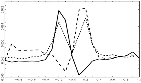
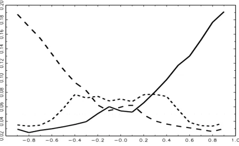
Figure 5:
Empirical rejection frequency of unit-root null hypotheses using HEGY t–and F–tests for 200 observations at nominal 5% significance level. Solid curve for t1, long dashes for t2, and short dashes for F34. Generating model is ∆4yt=φ∆4yt−1+εt with N(0,1) errors εt,φon the abscissa axis, 10000 replications.