IHS Economics Series Working Paper 261
January 2011
A Simple Panel-CADF Test for Unit Roots
Mauro Costantini
Claudio Lupi
Impressum Author(s):
Mauro Costantini, Claudio Lupi Title:
A Simple Panel-CADF Test for Unit Roots ISSN: Unspecified
2011 Institut für Höhere Studien - Institute for Advanced Studies (IHS) Josefstädter Straße 39, A-1080 Wien
E-Mail: o ce@ihs.ac.atffi Web: ww w .ihs.ac. a t
All IHS Working Papers are available online: http://irihs. ihs. ac.at/view/ihs_series/
This paper is available for download without charge at:
https://irihs.ihs.ac.at/id/eprint/2035/
A Simple Panel-CADF Test for Unit Roots
Mauro Costantini, Claudio Lupi
261
Reihe Ökonomie
Economics Series
261 Reihe Ökonomie Economics Series
A Simple Panel-CADF Test for Unit Roots
Mauro Costantini, Claudio Lupi January 2011
Institut für Höhere Studien (IHS), Wien
Institute for Advanced Studies, Vienna
Contact:
Mauro Costantini Department of Economics University of Vienna Bruenner Strasse 72 1210 Vienna, Austria
email: mauro.costantini@univie.ac.at Claudio Lupi – corresponding author University of Molise
Faculty of Economics Dept. SEGeS Via De Sanctis
I-86100 Campobasso, Italy Fax +39 0874 311124
: +39 0874 404451 email: lupi@unimol.it
Founded in 1963 by two prominent Austrians living in exile – the sociologist Paul F. Lazarsfeld and the economist Oskar Morgenstern – with the financial support from the Ford Foundation, the Austrian Federal Ministry of Education and the City of Vienna, the Institute for Advanced Studies (IHS) is the first institution for postgraduate education and research in economics and the social sciences in Austria. The Economics Series presents research done at the Department of Economics and Finance and aims to share “work in progress” in a timely way before formal publication. As usual, authors bear full responsibility for the content of their contributions.
Das Institut für Höhere Studien (IHS) wurde im Jahr 1963 von zwei prominenten Exilösterreichern – dem Soziologen Paul F. Lazarsfeld und dem Ökonomen Oskar Morgenstern – mit Hilfe der Ford- Stiftung, des Österreichischen Bundesministeriums für Unterricht und der Stadt Wien gegründet und ist somit die erste nachuniversitäre Lehr- und Forschungsstätte für die Sozial- und Wirtschafts- wissenschaften in Österreich. Die Reihe Ökonomie bietet Einblick in die Forschungsarbeit der Abteilung für Ökonomie und Finanzwirtschaft und verfolgt das Ziel, abteilungsinterne Diskussionsbeiträge einer breiteren fachinternen Öffentlichkeit zugänglich zu machen. Die inhaltliche Verantwortung für die veröffentlichten Beiträge liegt bei den Autoren und Autorinnen.
Abstract
In this paper we propose a simple extension to the panel case of the covariate-augmented Dickey Fuller (CADF) test for unit roots developed in Hansen (1995). The extension we propose is based on a p-values combination approach that takes into account cross-section dependence. We show that the test is easy to compute, has good size properties and gives power gains with respect to other popular panel approaches. A procedure to compute the asymptotic p-values of Hansen’s CADF test is also a side-contribution of the paper. We also complement Hansen (1995) and Caporale and Pittis (1999) with some new theoretical results. Two empirical applications are carried out for illustration purposes on international data to test the PPP hypothesis and the presence of a unit root in international industrial production indices.
Keywords
Unit root, Panel data, Approximate P-values, Monte Carlo
JEL Classification
C22, C23, F31
Contents
1 Introduction 1
2 The CADF test and the p-values approximation 4 3 The inverse normal combination test 8 4 Monte Carlo simulations 10
4.1 Structure of the DGP ... 11 4.2 Parameters setting and experimental design ... 15 4.3 Simulation results ... 18
5 The size of panel vs individual tests 36
6 Applications 38
6.1 Testing the PPP hypothesis ... 38 6.2 Unit roots in international industrial production indices ... 39
7 Concluding remarks 40
Acknowledgements 41
References 41 Appendix A:
The algorithm to compute the p-values of the CADF test 45
1 Introduction
It is well known that standard unit root tests suffer from low power (see e.g.Campbell and Perron, 1991; DeJonget al., 1992; Phillips and Xiao, 1998). Starting from the mid- nineties, it has been suggested that a viable way to increase power in unit root testing is to exploit cross-section variation together with univariate time series dynamics (seeQuah, 1994; Levin et al., 2002, among others). Panel unit root tests have become increasingly popular ever since. Of course, potential power gains are not the only reason for using panel tests. A commonly neglected advantage of the panel unit root approach is that it can be useful in avoiding some complications arising from multiple testing, as we will show in this paper. Furthermore, some specific cross-country macroeconomic analyses may fit naturally in the panel framework, in particular when the focus is on testing for the presence of a unit root as an interesting economically interpretable common feature in a whole set of time series. However, the power gain motivation has probably been the dominating one in the majority of theoretical and applied papers and it has been questioned only recently (see e.g.Banerjeeet al.,2004,2005).
In order to obtain more powerful unit root tests, Hansen(1995) adopted a different approach to exploit cross-sectional correlation. Rather than using panel data on a single variable,Hansen(1995) suggested using stationary covariates in an otherwise standard Dickey-Fuller framework, in this way proposing his covariate augmented Dickey-Fuller test (CADF). Indeed, Hansen (1995) and Caporale and Pittis (1999) showed that sub- stantial power gains can be achieved using the CADF test, without incurring severe size distortions.
In this paper we couple the two approaches, extendingHansen’s CADF test to small panels. AlthoughHansen(1995) is the seminal paper concerning covariate-augmented unit root tests, other tests might have been considered. In fact,Elliott and Jansson(2003) show thatHansen’s CADF test is not the point optimal test in general, and that feasible point optimal tests based on VAR models can be derived. However, we prefer to use the test proposed inHansen(1995) for three main reasons. First, simulations reported inEl- liott and Jansson(2003) show that the feasible point optimal tests can give power gains at the cost of inferior size performances: this is important in our framework, becauseHanck (2008) shows that size distortions tend to cumulate in panel tests of the kind proposed here. Second,Hansen’s CADF test is based on the familiar ADF framework, so that it can be more appealing to practitioners once the computational burden related to the compu- tation of the test p-values is eased. Finally, we show that under conditions considered as especially relevant for the panel unit root hypothesis, the CADF test is based on the correct conditional model.
The extension we propose is based on a p-value combination approach advocated independently inMaddala and Wu(1999) andChoi(2001). In this paper we refer mainly to Choi’s Z-test, that combines the p-values computed from unit root tests applied to each time series in the panel using an inverse-normal formulation. The method is well grounded in the meta-analytic tradition and its choice is supported by several reasons.
First, provided that we can compute the p-values of the CADF test, the extension to the panel case is straightforward: the panel test is very easy to compute and intuitive and practitioners can track without difficulty what is going on step-by-step in the analysis, from the univariate to the panel case. Second, the asymptotics carries through for the temporal sizeT →∞, without requiring also the number of cross-section unitsN →∞as other approaches instead do: in our view, given that allowingN → ∞in typical macro- panel applications is an implausible hypothesis, this is an extremely important feature of the tests based on Choi (2001). In fact, the test we propose here is especially well suited for small to moderate values ofN. Third, we don’t need balanced panel data sets, so that individual time series may come in different lengths and span different sample periods: this can be very useful in practice for example when data from many different countries have to be utilized. However, when data come from a balanced macro panel, quite natural stationary covariates can be used for each equation, as suggested inPesaran (2007) andChang and Song(2009). Fourth, the test allows for heterogeneous panels: the stochastic as well as the non stochastic components can be different across individual time series. Last, the alternative hypothesis doesn’t have to be that all the individual time series are stationary: the alternative that considers that some individual time series have a unit root and others do not can be dealt with by using the tests built uponChoi (2001). Indeed, we deliberately deal with the null hypothesis that all of the series in the panel are I(1) against the alternative thatat least one of the series is I(0). In fact, this hypothesis is common to most tests for a unit root in panels. Some authors consider this as a disadvantage (seeTaylor and Sarno,1998, among others), but we believe that the extent to which this is a real limitation depends on the specific goal of the analysis.
On the other hand, a potentially serious drawback of the methodology advocated in Choi(2001) is that it is based on the hypothesis that the individual time series are cross- sectionally independent. Indeed, this is a common assumption of many papers dealing with panel unit roots and panel cointegration (seeBanerjee,1999;Baltagi and Kao,2000;
Choi,2006, for comprehensive surveys). However, it is well known (see e.g.O’Connell, 1998; Maddala and Wu, 1999; Banerjeeet al.,2004,2005; Gengenbachet al., 2006;Lyha- gen, 2008; Wagner, 2008) that both short-term and long-run cross-section dependence adversely affects the performance of these panel unit roots tests. Therefore, we extend the approach to cross-sectionally dependent panel units by using the p-value correction method advocated inHartung(1999) andDemetrescuet al.(2006).1
Although developed independently, the results reported in the present paper are re- lated to other recent research. Despite some similarities, even in the name, the panel- CADF (pCADF) test presented here should not be confused with the cross-sectionally augmented ADF (CADF) test advocated inPesaran(2007).2 The CADF-CIPS test devel- oped byPesaranis explicitly derived with the aim of addressing directly the problem of
1Hartung’s correction has been utilized in other recent papers: see, among others,Hassler and Tarcolea (2005) andWesterlund and Costantini(2009).
2Notwithstanding the similarity of the names withPesaran’s test, we think that it is fair to refer to the originalHansen’s test using the original acronym CADF proposed byHansenhimself. In order to minimize confusion withPesaran’s test, we label our panel extension aspCADF.
cross-sectional dependence. AlsoPesaran’s test is related toHansen(1995), but model augmentation takes place using non-stationary covariates. Furthermore, differently from the pCADF test we propose here, in Pesaran (2007) the asymptotic results are derived under N → ∞, either with a fixed T or with T → ∞ sequentially or jointly with N.3 Chang and Song(2009) also start from the observation that using stationary covariates can greatly improve the power of unit root tests. However, the approach developed in Chang and Song(2009) is rather different from ours: while we use a simple p-value com- bination approach, Chang and Song (2009) propose a method based on non-linear IV estimation of the autoregressive coefficient, the suggested instruments being non-linear transformations of the lagged levels: this procedure should allow coping with cross- sectional dependencies of unknown form. In fact, Chang and Song (2009) show that the IV-based t-ratios associated with the autoregressive parameters are asymptotically independent even in the presence of cross-sectionally dependent time series. The test is proposed in three variants based on the average, the min, or the maxt-ratio, depending on the specific null and alternative hypothesis.4
The rest of the paper is organized as follows. Section2is devoted to a brief discussion of the test proposed inHansen(1995). We also illustrate the method we use to obtain the necessary p-values.5 Indeed, this is a subsidiary, but we believe important, contri- bution of this paper. In fact, while critical values ofHansen’s test are readily available fromHansen(1995), to the best of our knowledge, no other procedure has been proposed so far for the numerical computation of the test p-values. Section3is devoted to a brief account of the inverse normal combination method and its modifications to deal with dependent time series. In Section4an extensive Monte Carlo analysis of thepCADF test is carried out. The Data Generating Process (DGP) we propose in the paper encompasses other DGPs that are commonly used in the panel unit root literature and it is also related to the DGP used inHansen(1995). Beside giving us more flexibility in the design of the experiments, our DGP allows us to complementHansen(1995) andCaporale and Pittis (1999) with new theoretical results and interpretations of the simulations outcomes. The performance of the pCADF test is compared to that of other important panel unit root tests, namely those advocated in Chang and Song(2009),Demetrescu et al. (2006) and Moon and Perron(2004). All these tests allow for cross-dependence and share the same null and alternative hypothesis. In Section5we show that when the null hypothesis is H0 : “all of the series are I(1)” and the alternative is H1 : “at least one series is I(0)”, repeated application of individual unit root tests generates huge size distortions. This is an often neglected reason to prefer panel tests in such circumstances. For the purpose of illustration, in Section6we apply ourpCADF test to the PPP hypothesis and to interna-
3However,Pesaran(2007) shows that satisfactory size and power properties can be obtained even for rather small values ofN.
4In factChang and Song(2009) consider three different formulations of the unit root hypothesis: (A) H0: all of the series areI(1)against H1: all of the series areI(0); (B) H0: all of the series areI(1)against H1: at least one of the series isI(0); (C) H0: some of the series areI(1)against H1: all of the series areI(0).
5The algorithm to derive the p-values is described in detail in Appendix A. TheR(?) packageCADFtest (Lupi,2009) that computesHansen’s test and its p-values can be freely downloaded from the Comprehensive RArchive Network (CRAN) atwww.cran.r-project.org/package=CADFtest.GAUSSprocedures to compute Hansen’s test p-values are available from the authors upon request.
tional industrial production indices. The last Section concludes. An Appendix describes the algorithm used to compute the p-values ofHansen’s test.
2 The CADF test and the p-values approximation
The CADF test proposed inHansen(1995) starts from the idea that real economic phe- nomena are not univariate in general. Therefore, using extra information in unit root testing can make test regressions more efficient, allowing more precise inferences.
Formally,Hansen(1995) assumes that the seriesytto be tested for a unit root can be written as
yt = dt+st (1)
a(L)∆st = δst−1+vt (2)
vt = b(L)0(∆xt−µx) +et (3) where dt is a deterministic term (usually a constant or a constant and a linear trend), a(L) := (1−a1L−a2L2−. . .−apLp)is a polynomial in the lag operator L, xtis an m- vector,µx := E(∆x), b(L) := (bq2L−q2+. . .+bq1Lq1)is a polynomial where both leads and lags are allowed. Furthermore, consider the long-run covariance matrix
Ω :=
∑
∞ k=−∞E
"
vt et
!
vt−k et−k
#
= ω
v2 ωve ωve ω2e
!
(4) and define the long-run squared correlation betweenvtandetas
ρ2:= ω
2ve
ω2vωe2. (5)
When∆xt explains nearly all the zero-frequency variability of vt, thenρ2 ≈ 0. On the contrary, when∆xthas no explicative power on the long-run movement ofvt, thenρ2 ≈ 1. Furthermore, as emphasized byHansen(1995, p. 1151), whenet is uncorrelated with
∆xt−k ∀k, thenρ2 = ω2e/ω2v. The caseρ2 = 0 is ruled out (Hansen,1995, p. 1151), which implies thatytandxtcannot be cointegrated.
Similarly to the conventional ADF test, the CADF test is based on three different mod- els representing the “no-constant”, “with constant”, and “with constant and trend” case, respectively
a(L)∆yt = δyt−1+b(L)0∆xt+et (6) a(L)∆yt = µ+δµyt−1+b(L)0∆xt+et (7) a(L)∆yt = µ∗+θt+δτyt−1+b(L)0∆xt+et (8) and is computed as thet-statistic forδ,td(δ).Hansen(1995, p. 1154) proves that under the
unit-root null, the asymptotic distribution oftd(δ)in (6) is
td(δ)−→w ρ R1
0 W dW
R1
0 W21/2 + 1−ρ21/2
N(0, 1) (9)
whereW is a standard Wiener process and N(0, 1)is a standard normal independent of W. Therefore, the asymptotic distribution is a weighted sum of a Dickey-Fuller and a standard normal distribution. As a consequence, if ρ2 6= 1, conventional ADF critical values would lead to a conservative test.
The asymptotic distribution of the test statistic depends on the nuisance parameter ρ2but, providedρ2is given, it can be simulated using standard techniques. The mathe- matical expression remains unchanged if a model with constant (t[(δµ)) or a model with constant and trend (t[(δτ)) are considered, except that demeaned and detrended Wiener processes are used instead of the standard Wiener processW.
In order to extendHansen’s CADF unit root test to the panel case using the approach outlined inChoi(2001), we need to compute the p-values of the CADF unit root distribu- tion.
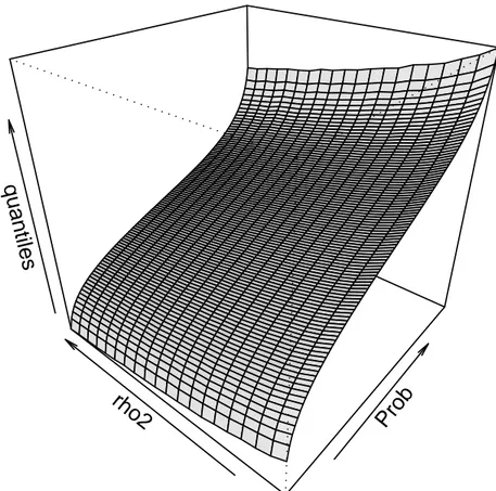
We derive the quantiles of the asymptotic distribution for different values ofρ2. Given that our goal is the computation of p-values, we simulate the distributions for 40 values ofρ2 (ρ2 = 0.025, 0.05, 0.0725, . . . , 1) using 100, 000 replications for each value ofρ2 and T=5, 000 as far as the Wiener functionals are concerned.6 From the simulated values we derive 1, 005 estimated asymptotic quantiles, (0.00025, 0.00050, 0.00075, 0.001, 0.002, . . . , 0.998, 0.999, 0.99925, 0.99950, 0.99975).
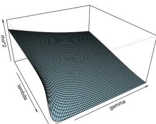
Figure1reports the estimated asymptotic quantiles for the model with constant, with- out any smoothing. The surface is extremely regular.7 Similar considerations carry over for the “no constant” and the “constant plus trend” cases. Therefore we expect that the simulated values can be successfully used to derive asymptotic p-values along lines sim- ilar toMacKinnon(1996).
In order to derive p-values from tabulated quantiles of a given distribution,MacKin- non(1996, p. 610) proposed using a local approximation of the kind
Φ−1(p) =γ0+γ1qd(p) +γ2qd(p)2+γ3qd(p)3+νp (10) where Φ−1(p) is the inverse of the cumulative standard normal distribution function evaluated atp andqd(p)is the estimated quantile.8 Equation (10) is not estimated glob- ally (as one would do with a standard response surface). Rather, it is estimated only over a relatively small number of points, in order to obtain alocal approximation (see MacKinnon,1996, p. 610, for details).
With respect toMacKinnon(1996), we have the extra difficulty that we have to deal
6Simulations have been carried out usingR(see?).
7Figure1reports the estimated asymptotic quantiles using a coarser resolution than the one used in the computations.
8InMacKinnon(1996) approximate finite sample quantiles are used, instead of the asymptotic ones.
Prob rho2
quantiles
Figure 1– Estimated asymptotic quantiles oft[(δµ).
ρρ2
0 0.2 0.4 0.6 0.8 1
−2.8−2.4−2.0
ρρ2
0 0.2 0.4 0.6 0.8 1
−2.6−2.2−1.8
ρρ2
0 0.2 0.4 0.6 0.8 1
−0.50.00.51.0
ρρ2
0 0.2 0.4 0.6 0.8 1
0.00.51.0
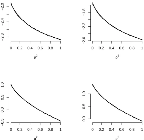
Figure 2– Interpolation of the quantilesq[ρ(p). From upper-left clockwise: α = 5%, α = 10%,α = 95%,α = 90%. The thick solid lines are the simulated quantiles. The thin lines are the interpolated values.
Standard Demeaned Detrended
ρ2 1% 5% 10% 1% 5% 10% 1% 5% 10%
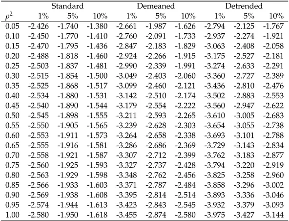
0.05 -2.426 -1.740 -1.380 -2.661 -1.987 -1.626 -2.794 -2.125 -1.767 0.10 -2.450 -1.770 -1.410 -2.760 -2.091 -1.733 -2.937 -2.274 -1.921 0.15 -2.470 -1.795 -1.436 -2.847 -2.183 -1.829 -3.063 -2.408 -2.058 0.20 -2.488 -1.818 -1.460 -2.924 -2.266 -1.915 -3.175 -2.527 -2.181 0.25 -2.503 -1.837 -1.481 -2.990 -2.339 -1.991 -3.274 -2.633 -2.291 0.30 -2.515 -1.854 -1.500 -3.049 -2.403 -2.060 -3.360 -2.727 -2.389 0.35 -2.525 -1.868 -1.517 -3.099 -2.460 -2.121 -3.436 -2.810 -2.476 0.40 -2.534 -1.880 -1.531 -3.142 -2.510 -2.174 -3.502 -2.883 -2.553 0.45 -2.540 -1.890 -1.544 -3.179 -2.554 -2.222 -3.560 -2.947 -2.622 0.50 -2.545 -1.898 -1.555 -3.211 -2.593 -2.265 -3.610 -3.005 -2.683 0.55 -2.550 -1.905 -1.565 -3.239 -2.628 -2.303 -3.654 -3.055 -2.738 0.60 -2.553 -1.911 -1.573 -3.264 -2.658 -2.338 -3.693 -3.101 -2.788 0.65 -2.555 -1.916 -1.581 -3.286 -2.686 -2.369 -3.729 -3.143 -2.834 0.70 -2.558 -1.921 -1.587 -3.307 -2.712 -2.399 -3.762 -3.183 -2.877 0.75 -2.560 -1.925 -1.593 -3.327 -2.737 -2.428 -3.794 -3.220 -2.919 0.80 -2.563 -1.929 -1.598 -3.348 -2.762 -2.456 -3.825 -3.258 -2.960 0.85 -2.566 -1.933 -1.603 -3.371 -2.787 -2.484 -3.858 -3.296 -3.002 0.90 -2.569 -1.938 -1.608 -3.395 -2.814 -2.514 -3.893 -3.336 -3.046 0.95 -2.574 -1.944 -1.613 -3.423 -2.843 -2.545 -3.932 -3.379 -3.093 1.00 -2.580 -1.950 -1.618 -3.455 -2.874 -2.580 -3.975 -3.427 -3.144
Table 1– Asymptotic critical values of the CADF test.
with the nuisance parameterρ2, so that the local approximation must be obtained along two dimensions. However, given that quantiles change fairly smoothly by varyingρ2, we adopt a rather straightforward two-step procedure. In the first step we interpolate the quantilesqd(p)to obtain an approximation for the relevant value ofρ2. In practice we use
q[ρ(p) =β0+β1ρ2+β2ρ4+β3ρ6+ερ (11) where we have used the subscriptρinq[ρ(p)to indicate the dependence of the quantiles onρ2. Interpolation is always very good, as can be gathered from Figure2.
As a by-product of our analysis, we compute a detailed table of asymptotic critical values of the CADF test using equation (11) (see Table1). Given that these critical values are based on a larger number of replications and on a response surface approach (see e.g.
Hendry,1984), we believe that they can be more accurate than those reported inHansen (1995).
Finally we apply the procedure advocated inMacKinnon(1996) on the interpolated quantiles to obtain the p-values.9
3 The inverse normal combination test
Once computation of the p-values for the distribution (9) is solved, the extension of Hansen’s test to the panel case is straightforward. Indeed, Choi(2001) shows that un-
der some fairly general regularity conditions, if the cross-section unitsi = 1, . . . ,N are independent, under the null
Z:= √1 N
∑
N i=1tbi −→w N(0, 1) (12)
where the bti’s are theprobits bti := Φ−1(pbi), with Φ(·)the standard normal cumulative distribution function, andpbi the estimated individual p-values fori=1, . . . ,N. Conver- gence in (12) takes place asT → ∞, whereas N < ∞ is the number of individual time series. T → ∞is required for the relevant statistics to converge to a proper continuous distribution, under some regularity conditions. The null hypothesis is H0 : δ = 0 ∀i, while the alternative is H1:δ <0 for at least onei, withi=1, 2, . . . ,N. This is a different alternative from H1 :δ<0∀i, used in other tests (see e.g.Levin and Lin,1993;Levinet al., 2002;Quah,1994). In fact, we believe that our formulation of the null and of the alterna- tive hypothesis is an advantage, rather than a disadvantage, as some authors claim: the null hypothesis that all of the series are I(1)against the alternative that all of the series areI(0)is not very interesting and informative, given that it can be tested only under the maintained hypothesis that the crucial parameter characterising the presence/absence of the unit root is homogeneous across the individual time series in the panel (see e.g.Levin et al.,2002). Also from the economist’s point of view there are instances in which it can be more interesting to test for a unit root collectively over a whole panel of time series because this can be interpreted as a stylized fact that can give stronger support in favour (or against) a particular economic interpretation as compared to the same analysis con- ducted separately on each single time series. Furthermore, because of the presence of multiple testing the two approaches are not statistically equivalent.
However, the presence of cross-section dependence among the time series compli- cates substantially the theoretical framework, and the test statistic is no longer asymptot- ically (withT) standard normal. However,Hartung(1999) suggests that a suitably mod- ified inverse normal combination test can be obtained. The advantage of this solution is that under the null the test statistic has approximately standard normal distribution even in the presence of correlated individual test outcomes. In particular,Hartung(1999) analyses the case where the pairwise correlation across the individual test statistics is constant and equal to$, say. If$were known then, given a setλi, . . . ,λN of real valued weights such that∑Ni=1λi 6=0, it would be possible to compute
t($):= ∑
Ni=1λibti r
(1−$)∑iN=1λ2i +$
∑iN=1λi
2 (13)
which under the null would be N(0, 1). When$ = 0 (no cross-section dependence) and λi =1∀i, then (13) collapses into (12).
Of course,$is not known, and the feasible test statistic advocated byHartung(1999,
p. 851) is
t($ˆ∗,κ):= ∑
Ni=1λitbi s
∑1N=1λ2i +
∑Ni=1λi 2
−∑iN=1λ2i
$ˆ∗+κ q 2
N+1(1−$ˆ∗)
(14)
where ˆ$∗ is a consistent estimator of $ such that ˆ$∗ = max{−1/(N−1), ˆ$}with ˆ$ = 1−(N−1)−1∑Ni=1(tbi−N−1∑iN=1bti)2.κ >0 is a parameter that controls the small sample actual significance level. Hartung (1999) shows that under the null t($ˆ∗,κ)is approxi- mately distributed as N(0, 1). However, the proof offered inHartung(1999) rests on the assumption that the probits are not only individually N(0, 1), but are also jointly multi- variate normal.
Demetrescu et al. (2006) generalize Hartung’s results in two directions. They first show that the pairwise correlation of the individual test statistics need not be constant for Hartung’s results to hold (Demetrescu et al.,2006, Proposition 1, p. 651). Furthermore, they wonder under what conditions does the inverse normal method map the original test statistics to a multivariate normal distribution of the probits and they conclude that the necessary and sufficient condition fort($)to have a standard normal distribution is that the test statistics from which the probits are derived are such to have the copula of a multivariate normal distribution (Demetrescuet al.,2006, Proposition 2, p. 653). Despite the fact that the augmented Dickey-Fuller test does not satisfy the condition stated in their Proposition 2,Demetrescuet al.(2006) suggest that correcting for dependence using (14) may still be a good practice because units cross-correlation is likely to have much stronger adverse effects on inference than deviations from normality of the individual test statistics can have. Indeed, they show by simulation that this is in fact the case.
In this paper we follow the approach suggested byDemetrescuet al.(2006) to com- bine the p-values of the individual CADF unit root tests in the presence of cross-section dependence. We argue that, if the correction proposed inHartung (1999) works quite nicely in the presence of Dickey-Fuller distributions, it shoulda fortioriwork at least as nicely in the presence of distributions that are closer to the standard normal. In other words, given that under the nullHansen’s distribution is precisely a weighted sum of a Dickey-Fuller and a standard normal distribution, we expect that the correction for cross-section dependence in our case should be at least as effective as it is in the standard Dickey-Fuller case explored byDemetrescuet al.(2006).
4 Monte Carlo simulations
In this Section we compare the performance of thepCADF test to that of three unit root tests that are valid under cross-dependence. Specifically, we compare our test with an ADF-based p-values combination test (Demetrescuet al.,2006), with a dynamic factor test (Moon and Perron,2004) and with a recent IV-based covariate-augmented test (Chang and Song,2009). For the latter two tests we consider in particular thet∗a statistic (Moon
pp. 905–906), respectively. All these tests share the same null H0 : “all of the series are I(1)” and the same alternative H1: “at least one series is I(0)”.
We verify the performances of thepCADF test and of the test proposed inDemetrescu et al.(2006) using the versions of the tests with constant and with constant and linear trend.10 The tests advocated inChang and Song(2009) andMoon and Perron(2004) are examined in both the demeaned and detrended versions.
4.1 Structure of the DGP
In our simulations we consider the following DGP:
∆yt = α+Dyt−1+ut (15) ut
ξt
!
= B γ
00 λ
! ut−1 ξt−1
!
+ ηt εt
!
(16) ηt
εt
!
∼ N
"
0 0
!
, Σ11 σ12 σ012 σ22
!#
(17) where∆is the usual difference operator,yt := (y1t, . . . ,yNt)0,ut := (u1t, . . . ,uNt)0,α := (α1, . . . ,αN)0,D:=diag(δ1, . . . ,δN),B :=diag(β1, . . . ,βN),γ := (γ1, . . . ,γN)0 andηt:= (η1t, . . . ,ηNt)0. Note that (16) defines a VAR(1) which is stationary as long as|βi| < 1∀i and|λ|<1.11 δi =0∀iunder the null, while under the alternativeδi <0 for somei.
We believe that the proposed DGP is especially interesting, because it can be viewed as a panel extension of the DGP proposed inHansen(1995, p. 1161) and at the same time is also a generalization of two DGPs commonly used in the panel unit root literature (see e.g.Chang and Song,2009;Phillips and Sul,2003). The two DGPs that are special cases of ours, whenα=0share the same equation (15) for∆yt, but differ as far as the simulation of theut’s is concerned:
DGP1: uit = βiui,t−1+νit (18)
DGP2: uit = βiui,t−1+γiζt+νit (19) where theN-vectorνtis i.i.d. N(0,Σ11)withΣ11 6= I andζt is a i.i.d. N(0, 1)common factor independent ofνt.
It can be seen that, even whenα =0, our DGP (15)–(17) is more general than both (18) and (19): in fact, in our DGP the “common factor”ξtcan be autocorrelated and non-zero correlations between the innovations toui,t and the innovations toξt can be introduced.
As a result, the cross-dependence structure is stronger than in either DGP1 or DGP2.
10We do not consider the models without deterministic terms that are less relevant in practical applica- tions.
11To see this, let’s define
Φ:=
B γ 00 λ
and note thatΦis upper-triangular, so that the eigenvalues ofΦare given simply by the diagonal elements ofΦ, dg(Φ). Therefore, the VAR(1) is stationary as long as|βi|<1∀iand|λ|<1.
However, DGP2 can be derived as a special case from (15)–(17) whenλ=0 andσ12 =0, while DGP1 is retrieved if in additionγ =0. In both cases, in generalΣ11 6=I.
Using the DGP (15)–(17) we can determine the form of the model that should be used to test for a unit root in each singleyit. For simplicity, assume nowα=0. Then, denoting the “past” byZt−1, the correct conditional model for∆yi,tis
E(∆yi,t|ξt,Zt−1) = δi(1−βi)yi,t−1+ (1+δi)βi∆yi,t−1 + (σ12)i
σ22 ξt+
γi−(σ12)i σ22 λ
ξt−1. (20) with(σ12)i thei-th element ofσ12. Note that (20) has the form of a CADF(1,1,0) model.
In fact, unlessγ = 0 andσ12 = 0, the standard approach of using a panel combination ADF test in a context where the DGP is supposed to be of the kind of (15)–(17) (which is a fairly standard situation in the panel unit root literature) is bound to be at least inefficient, because the correct models should includeξtand/orξt−1and the individual tests should be CADF. Even ifγi =0 (i.e., whenξtdoes not Granger-causeut), as far as(σ12)i 6=0 the correct model has the form of a CADF(1,1,0).
Expression (20) is very similar to an expression derived inCaporale and Pittis(1999, p. 586, equation 11) and some special cases can be of interest. Under DGP2 (λ = 0 and σ12=0) the correct conditional model becomes
E(∆yi,t|ξt,Zt−1) =δi(1−βi)yi,t−1+ (1+δi)βi∆yi,t−1+γiξt−1 (21) and we should expect the pCADF test to have a better performance than the tests based on the conventional ADF. Of course, the same conditional model (21) holds for thei-th unit if only(σ12)i =0, while ifλ=0 and(σ12)i 6=0 we have
E(∆yi,t|ξt,Zt−1) = δi(1−βi)yi,t−1+ (1+δi)βi∆yi,t−1
+ (σ12)i
σ22 ξt+γiξt−1. (22) On the other hand, under DGP1 (λ=0,σ12=0,γ=0), the correct conditional model is simply
E(∆yi,t|ξt,Zt−1) = δi(1−βi)yi,t−1+ (1+δi)βi∆yi,t−1 (23) which has the form of an ordinary ADF(1) test equation, so that in this case thepCADF test has no advantage on p-values combination tests based on the ADF test.
From the discussion in Section2, we know that the power of the CADF test depends crucially on the nuisance parameter ρ2. Therefore, the power of the pCADF tests will depend on the values of this parameter for each unit in the panel,ρ2i. Using the DGP (15)–(17) we can derive analytically the theoretical value of ρ2i under the DGP.12 This
12Hansen(1995) derivesρ2 by simulation using different models. None of the models used byHansen (1995, Table 3, p. 1162) correspond to the correctly specified CADF(1,1,0), so that all the models are either over- or under-parameterized. Using the theoretical results derived below jointly withHansen’s results, we
lambda
r rho^2
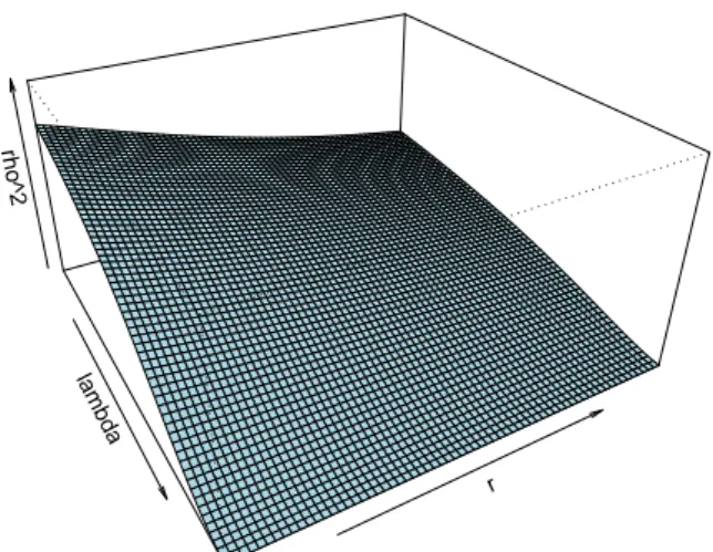
Figure 3– Values ofρ2for varying values of 0 < λ < 1 and 0 < ri < 1,γi = 0.5, σei =σε =1.ρ2is plotted on a 0−1 scale.
result gives important insights to better investigate the performance of the test in the Monte Carlo experiments.
Consider the residualei,tfrom the correct conditional model (20) ei,t = ∆yi,t−δi(1−βi)yi,t−1−(1+δi)βi∆yi,t−1
− (σ12)i σ22 ξt−
γi−(σ12)i σ22 λ
ξt−1. (24)
Given thatei,tis the residual from the correct conditional model, it must be an innovation uncorrelated with ξt−k ∀k. As discussed in Hansen (1995, p. 1151), in this case ρ2i = ω2ei/ω2vi withω2hthe long-run variance ofh, that is the zero-frequency spectral density of h(h∈ {ei, vi}). Given thatei,t is an innovation, its long-run variance is just the variance ofei,t, apart from the normalizing factor(2π)−1.
Now consider
vi,t = (σ12)i σ22 ξt+
γi−(σ12)i σ22 λ
ξt−1+ei,t. (25) In order to compute the long-run variance ofvi,t, ω2vi, from (16) note thatξt = (1− λL)−1εtand defineri := (σ12)i/σ22. Then, rewrite (25) as
vi,t = [ri+ (γi−riλ)L]ξt+ei,t
= ri+ (γi−riλ)L
1−λL εt+ei,t. (26)
can show that under-parameterization can result in biased estimates ofρ2, with adverse effects on inference.
This is particularly evident with respect toHansen’s experiments 11 and 15, where the simulation-based estimates ofρ2from the CADF(2,0,1) model are equal to 0.87 and 0.90, respectively, while the true values under the DGP are 0.67 and 0.50.
lambda
gamma rho^2
Figure 4– Values of ρ2 for varying values of 0 < λ < 1 and 0 < γi < 1,r = 0.5, σei =σε =1.ρ2is plotted on a 0−1 scale.
r
gamma rho^2
Figure 5– Values of ρ2 for varying values of 0 < r < 1 and 0 < γi < 1, λ = 0.5, σei =σε =1.ρ2is plotted on a 0−1 scale.
The spectral density ofvi,tat frequencyωis fvi(ω)∝
ri+ (γi−riλ)e−iω
2
|1−λe−iω|2 σ
2
ε +σe2i (27)
so that the long-run variance ofvi,t,ωv2i, is
ω2vi := fvi(0)∝ [γi+ (1−λ)ri]2 (1−λ)2 σ
2
ε +σe2i. (28)
Finally,ρ2i is given by
ρ2i = ω
2ei
ω2vi = σ
e2i
[γi+(1−λ)ri]2
(1−λ)2 σε2+σe2i
. (29)
The value ofρ2i is a nonlinear function of(σ12)i,σ22, γi andλ. Contrary to what is sug- gested inHansen(1995, p. 1161), we find that the value ofλis crucial in determining the value of the nuisance parameterρ2, also when the VAR(1) (16) is stationary. Of course, whenλ → 1, then ωv2i → ∞ andρ2 → 0: this is an expected result, because ifλ = 1, ξt has a unit root and is cointegrated with yi,t. Conversely, if γi = 0 and ri = 0, then ρ2i =1: in this case there would be no advantage in using individual CADF tests instead of standard ADF tests. Under DGP2, given thatλ = 0 andri = 0, ρ2i simply varies in- versely withγi. Under DGP1, where it is alsoγi = 0∀i, thenρ2i = 1∀iand the power of thepCADF test is substantially the same as the power of the test based onDemetrescu et al.(2006), consistently with what already pointed out while discussing the conditional model.
In (29) the larger are eitherλ,γi orri, the smaller isρ2i. Given that the power of the CADF test is higher the smaller is the value ofρ2i, this in turn defines the regions where the test is expected to perform better. A graphical summary of the relation betweenρ2i and the values ofλ,γi andri is offered in Figures3–5.
4.2 Parameters setting and experimental design
Some care must be exerted in simulating the DGP (15)–(17), especially as far as the simu- lation of(η0t,εt)0is concerned. From (17),(ηt0,εt)0 ∼N(0,Σ), with
Σ = Σ11 σ12 σ012 σ22
!
. (30)
We assume diag(Σ) := ı, withı := (1, . . . , 1)so that the generic element ofσ12,(σ12)i, coincides withri. However, we have to distinguish two different settings for Σ11, de- pending onσ12=0orσ126=0.
When σ12 = 0 (e.g. under DGP1 and DGP2), then we must generate the correla- tion matrix Σ11 in a way that is as flexible and unrestricted as possible. At the same time we want to introduce fairly strong dependence. Therefore, we start by generating a symmetric matrixΣ∗ whose diagonal elements are equal to 1 and whose non-diagonal
elements are randomly drawn from U(0,0.8). Of course, although symmetric,Σ∗is not in general positive definite. Therefore, we find a positive definite symmetric matrixΣ†that is “close” toΣ∗ by computingΣ† = V∗Λ†V∗0where the matrixV∗ is derived from the singular value decomposition ofΣ∗ andΛ†is the diagonal matrix of the eigenvalues of Σ∗, after substituting the negative eigenvalues with very small but positive values. Fi- nally, the positive definite covariance matrix obtained in this way (the diagonal elements are not exactly equal to one) is transformed into the required correlation matrixΣ11by normalization.13 The resulting symmetric positive definite matrixΣ11is such that most of the simulated correlations are positive, as we probably would expect in many empir- ical macro panel settings, and the average correlation is larger than the one simulated using the method proposed byChang(2002) andChang and Song(2009).14Furthermore, the simulatedΣ11is likely to satisfy Proposition 1 inDemetrescuet al.(2006).
On the other hand, whenσ12 6=0the parametersri := (σ12)i enter the expression for ρ2i and are therefore important design parameters that we want to control precisely. In this case we want to simulate a correlation matrixΣ whose last column is a given vector (σ120 , 1)0. Furthermore, given the vector of correlations σ12, it is reasonable to consider Σ11 6=I. However,Σ11in this case must be consistent with the givenσ12. Therefore, we introduce a minimal structure inΣ11 by assuming that its generic off-diagonal element is(Σ11)ij := (σ12)i(σ12)j (withi 6= j) and diag(Σ11) := ı. This structure essentially states that the moreηit is correlated withεt andηjt is correlated withεt, the moreηit is correlated withηjt, that is what we should expect in the usual case. Simulating such aΣ is very easy: just draw the elements ofσ12 from a specified distribution, U(rmin,rmax), say, and computeS =σ12σ120 . Set diag(S):=ıand callΣ11the resulting matrix. Then, build the correlation matrixΣ as in (30). The matrix Σ simulated in this way is symmetric positive definite.15
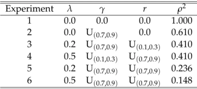
As already pointed out in the previous subsection, we expect the nuisance parameter ρ2 to influence the performance of our test. Therefore, rather than embarking in a full factorial design, we concentrate on just a few experiments carefully selected in such a way that they differ in the underlying value ofρ2(see Table2).
13The proposed algorithm is essentially equivalent to the procedure advocated inRebonato and J¨ackel (1999, Section 3).
14In a pilot simulation carried out using 50,000 replications we found that the average non-diagonal ele- ment of a 20×20 simulated correlation matrix was about 0.34 with the simulated correlations spanning the interval(−0.30, 0.96). We also used the procedure outlined inDemetrescuet al.(2006, p. 659). The results are very similar to those reported here and are available from the authors upon request.
15To see this, note thatΣ is real symmetric by construction. Then there exists a matrix P such that P0ΣP =Λ, withΛthe diagonal matrix of the eigenvalues ofΣ. P andΛcan be found using the Schur canonical form:
I −σ12 00 1
Σ11 σ12 σ120 1
I 0
−σ120 1
=
Σ11−σ12σ120 0
00 1
=
1−(σ12)21 0 . . . 0 0
0 1−(σ12)22 . . . 0 0
... ... . .. ... ...
0 0 . . . 1−(σ12)2N 0
0 0 . . . 0 1
=Λ.
Experiment λ γ r ρ2
1 0.0 0.0 0.0 1.000
2 0.0 U(0.7,0.9) 0.0 0.610
3 0.2 U(0.7,0.9) U(0.1,0.3) 0.410 4 0.5 U(0.1,0.3) U(0.7,0.9) 0.410 5 0.2 U(0.7,0.9) U(0.7,0.9) 0.236 6 0.5 U(0.7,0.9) U(0.7,0.9) 0.148
Table 2– Parameters setting. The values ofρ2are computed using the means of the Uniform distributions.
The other parameters of the DGP are generated as inChang and Song(2009): in par- ticular,βi ∼U(0.2,0.4)andγi ∼U(0.5,3)(withi=1, . . . ,N). Under the nullδi =0∀i, under the alternativeδi ∼ U(−0.2,−0.01)for the stationary units. In order to highlight the power of the tests when only a few series are stationary, the number of stationary units under the alternative is limited to 2.
Given that our DGP allows for a non-zero driftαi, we run the experiments first using αi =0∀iand then usingαi ∼U(0.7,0.9).
Finally, the experiments are carried out using 2,500 replications with T ∈ {100, 300} andN∈ {10, 20}that are fairly typical values in macro-panel applications.
Since the use of the pCADF test implies a sequence of decisions, we use a pseudo- real setting that aims at replicating the way these decisions might be taken in practice.
Therefore, the choice to correct or not to correct for cross-unit dependence is based on a test for the presence of cross-unit correlation (Pesaran,2004). When the test rejects the absence of correlation among the cross-section units, the panel test is performed by us- ing the modified weighted inverse normal combination (14), otherwise standard inverse normal combination (12) is utilized. When the modified version (14) is used, consistently withHartung(1999) andDemetrescu et al.(2006), in our experiments we useλi = 1 ∀i andκ = 0.2. Furthermore, the selection of the lags structure for the lagged differences of both the dependent variable and the covariate in the pCADF test equations (6)-(8) is based on the BIC separately for each equation. The choice of the variable to be used as the stationary covariate in testing the unit root for thei-th series in the panel is determined using three different criteria. First, the “true” covariate is used; second, we consider as the stationary covariate the average of the differenced series∆yjt (∀j 6= i)related to the other units in the panel, as inChang and Song(2009); third, we use the first difference of the first principal component of the series. A word of caution is in order here. It could be argued that selecting the stationary covariate using the average of the other∆yjtor the differences of the first principal component of the series may overlook the problem that the derived covariate might be non-invertible. In fact,Hansen(1995) showed that over- differencing the covariates raises theoretical problems and can have some adverse effects on the size and power of the test. However, for this to be the case it would be necessary that all the series areI(0). In this instance the test would have high power anyway.
The panel-ADF test is carried out in the version proposed byDemetrescuet al.(2006), that exploits the correction for cross-section dependence introduced byHartung(1999).