A Fixed-b Perspective on the Phillips-Perron Unit Root Tests

IHS Economics Series Working Paper 272

July 2011

A Fixed-b Perspective on the Phillips-Perron Unit Root Tests

Timothy J. Vogelsang

Martin Wagner

Impressum Author(s):

Timothy J. Vogelsang, Martin Wagner Title:

A Fixed-b Perspective on the Phillips-Perron Unit Root Tests ISSN: Unspecified

2011 Institut für Höhere Studien - Institute for Advanced Studies (IHS) Josefstädter Straße 39, A-1080 Wien

E-Mail: o ce@ihs.ac.atffi Web: ww w .ihs.ac. a t

All IHS Working Papers are available online: http://irihs. ihs. ac.at/view/ihs_series/

This paper is available for download without charge at:

https://irihs.ihs.ac.at/id/eprint/2081/

A Fixed-b Perspective on the Phillips-Perron Unit Root Tests

Timothy J. Vogelsang, Martin Wagner

272

Reihe Ökonomie

Economics Series

272 Reihe Ökonomie Economics Series

A Fixed-b Perspective on the Phillips-Perron Unit Root Tests

Timothy J. Vogelsang, Martin Wagner July 2011

Institut für Höhere Studien (IHS), Wien

Institute for Advanced Studies, Vienna

Contact:

Timothy J. Vogelsang Department of Economics Michigan State University 310 Marshall-Adams Hall East Lansing

MI 48824-1038, USA email: tjv@msu.edu Martin Wagner

Department of Economics and Finance Institute for Advanced Studies Stumpergasse 56

1060 Vienna, Austria

: +43/1/599 91-150

email: martin.wagner@ihs.ac.at and

Frisch Centre for Economic Research Oslo

Founded in 1963 by two prominent Austrians living in exile – the sociologist Paul F. Lazarsfeld and the economist Oskar Morgenstern – with the financial support from the Ford Foundation, the Austrian Federal Ministry of Education and the City of Vienna, the Institute for Advanced Studies (IHS) is the first institution for postgraduate education and research in economics and the social sciences in Austria. The Economics Series presents research done at the Department of Economics and Finance and aims to share “work in progress” in a timely way before formal publication. As usual, authors bear full responsibility for the content of their contributions.

Das Institut für Höhere Studien (IHS) wurde im Jahr 1963 von zwei prominenten Exilösterreichern – dem Soziologen Paul F. Lazarsfeld und dem Ökonomen Oskar Morgenstern – mit Hilfe der Ford- Stiftung, des Österreichischen Bundesministeriums für Unterricht und der Stadt Wien gegründet und ist somit die erste nachuniversitäre Lehr- und Forschungsstätte für die Sozial- und Wirtschafts- wissenschaften in Österreich. Die Reihe Ökonomie bietet Einblick in die Forschungsarbeit der Abteilung für Ökonomie und Finanzwirtschaft und verfolgt das Ziel, abteilungsinterne Diskussionsbeiträge einer breiteren fachinternen Öffentlichkeit zugänglich zu machen. Die inhaltliche Verantwortung für die veröffentlichten Beiträge liegt bei den Autoren und Autorinnen.

Abstract

We extend fixed-b asymptotic theory to the nonparametric Phillips-Perron (PP) unit root tests. We show that the fixed-b limits depend on nuisance parameters in a complicated way.

These non-pivotal limits provide an alternative theoretical explanation for the well known finite sample problems of PP tests. We also show that the fixed-b limits depend on whether deterministic trends are removed using one-step or two-step approaches, contrasting the asymptotic equivalence of the one- and two-step approaches under a consistency approximation for the long run variance estimator. Based on these results we introduce modified PP tests that allow for fixed-b inference. The theoretical analysis is cast in the framework of near-integrated processes which allows to study the asymptotic behavior both under the unit root null hypothesis as well as for local alternatives. The performance of the original and modified tests is compared by means of local asymptotic power and a small simulation study.

Keywords

Nonparametric kernel estimator, long run variance, detrending, one-step, two-step

JEL Classification

C12, C13, C32

Comments

The authors acknowledge financial support from the Jubiläumsfonds of the Oesterreichische National- bank (Grant Nr. 13398).

Contents

1 Introduction 1

2 The Fixed-b Limits of the Phillips-Perron Tests 1

2.1 One-Step Approach ... 2 2.2 Two-Step Approach ... 3 2.3 Asymptotic Results ... 4

3 Modified PP Unit Root Tests 6 4 Finite Sample Behavior 9 5 Summary and Conclusions 11 6 Appendix: Proofs 12

References 14

Figures 15

1 Introduction

In this paper we extend the fixed-b asymptotic theory of Kiefer and Vogelsang (2005) to the well known unit root tests of Phillips and Perron (1988), i.e. the PP tests. We focus on the case where PP tests are constructed using nonparametric kernel estimators of the long run variance. We find that the fixed-b limits of the PP tests are not pivotal and furthermore also depend on whether deterministic trends are removed using one-step or two-step detrending methods. Our results are in contrast to existing results based on consistency of the long run variance estimator in which case the asymptotic distributions of the PP tests are pivotal and are the same for one- and two- step detrending. Our finding of a non-pivotal fixed-b limit provides an alternative explanation for the often inadequate finite sample performance of PP tests (Perron and Ng, 1996 and Schwert, 1989). We propose a simple adjustment to the PP tests that provides a pivotal fixed-blimit under the unit root null. The theoretical analysis is performed using the framework of near-integrated process (cf. Phillips, 1987) which allows the derivation of limiting distributions both under the unit root null hypothesis as well as under local alternatives (to study local asymptotic power).

The remainder of the paper is organized as follows. In the next section we provide the fixed-b limits of the one- and two-step detrended versions of the PP tests. In Section 3 we propose the adjustment that restores an asymptotically pivotal limit. Section 4 provides some limited finite sample results and Section 5 briefly summarizes and concludes. All proofs are relegated to the appendix. Supplementary material available upon request provides fixed-b critical values for five kernel functions (Bartlett, Bohman, Daniell, Parzen and Quadratic Spectral), for the specification without deterministic components, with intercept only and with intercept and linear trend. For the latter two specifications of the deterministic component, critical values are available for both one- and two-step detrending.

2 The Fixed-b Limits of the Phillips-Perron Tests We assume that the data are generated according to

y_t=D⁰_tθ+y_t⁰, t= 1, . . . , T, (1) y⁰_t = (1− c

T)y⁰_t−1+u_t, (2)

whereD_t= [1, t, t², . . . , t^q]⁰ for some 0≤q <∞. When c= 0,y_t⁰ is a unit root process and values of c > 0 correspond to near-integrated (in the terminology of Phillips, 1987) stationary (for fixed T) alternatives.

The key assumption is that the process utsatisfies a functional central limit (FCLT), i.e.

T^−1/2

[rT]

X

t=1

ut⇒ωW(r), (3)

1

where [rT] is the integer part of rT with r ∈ [0,1], W(r) is a standard Wiener process and 0< ω²<∞is the long run variance ofu_t. Assuming for notational simplicity thatu_tis covariance stationary with summable autocovariance function, γj, we have

ω²=γ0+ 2

∞

X

j=1

γj. (4)

As is common, we use σ² to denote γ₀ and we furthermore define the half long run variance λ:= ¹₂(ω²−σ²).¹ Sufficient conditions for the FCLT can be found in Phillips and Solo (1992), or more specifically also in Phillips and Perron (1988) and in Simset al. (1990) who consider similar deterministic components as we do. It is well known (see Phillips 1987) that given (2) and (3) it follows that

T^−1/2y_[rT⁰ _]⇒ωV_c(r), whereV_c(r) =Rr

0 e^−c(r−s)dW(s).

Before we can turn to the analysis of the tests’ asymptotic behavior we need to define several additional quantities. DefineD(r) := [1, . . . , r^q]⁰ and define the correspondingly detrended process, Vec(r), and generalized Brownian bridge,Wc(r), as:

Vec(r) :=Vc(r)−D(r)⁰ Z 1

0

D(s)D(s)⁰ds

⁻¹Z 1 0

D(s)Vc(s)ds, (5)

cW(r) :=W(r)− Z r

0

D(s)⁰ds Z 1

0

D(s)D(s)⁰ds

⁻¹Z 1 0

D(s)dW(s). (6)

A slight variant ofVe_c(r) is also needed and is defined as e˙

V_c(r) :=W(r)− Z r

0

D(s) +˙ cD(s)0

ds Z 1

0

D(s)D(s)⁰ds

⁻¹Z 1 0

D(s)V_c(s)ds, where ˙D(r) = ^∂D(r)_∂r = [0,1,2r, . . . , qr^q−1]⁰. Note that Rr

0 D(s)ds˙ = [0, r, r², . . . , r^q]⁰ is simplyD(r) with its first element replaced with 0. For the pure unit root case,c= 0, because V₀(r) =W(r), it follows that Ve₀(r) and Ve˙₀(r) are similar but different stochastic processes. As we shall see below this difference is the effect of using either one- or two-step detrending.

In the rest of the paper we will use throughout a subscripti= 1,2 to refer to quantities related to either one- or two-step detrending, e.g. eyt,1 refers to the one-step detrended yt.

2.1 One-Step Approach

The one-step approach is based on estimating the regression model

y_t=D⁰_tδ+αyt−1+u_t, t= 2, . . . , T, (7)

1In case ut is not assumed to be stationary ω² and σ² are defined as ω² := limT→∞E 1

T(PT t=1ut)²

and σ²:= limT→∞ 1

T

PT

t=1E(u²t), compare Phillips and Perron (1988).

2

with the null hypothesis of interest being H₀ : α = 1. Using the Frisch-Waugh theorem the deterministic components can be eliminated and one can focus on the regression

ey_t,1=αyet−1,1+eu_t, t= 2, . . . , T, (8)

with ye_t,1 := y_t − D_t⁰(D_T⁰ D_T)⁻¹D⁰_TY_T, eyt−1,1 := yt−1 − D_t⁰(D_T⁰ D_T)⁻¹D⁰_TY_T−1 and eu_t := u_t − D⁰_t(D⁰_TDT)⁻¹D⁰_TUT, using the notationYT := [y2, . . . , yT]⁰,YT−1 := [y1, . . . , yT−1]⁰,UT := [u2, . . . , uT]⁰ and D_T := [D2, . . . , D_T]⁰.

The one-step PP unit root tests are based on the OLS estimator αb₁ :=

PT

t=2eyt,1eyt−1,1

PT

t=2ey_t−1,1² of α from (8), respectively thet-statistic

tα1 := αb1−1 q

σb²(PT

t=2ye_t−1,1² ) ,

with σb² := _T¹ PT

t=2bu²_t,1 and ubt,1 := yet,1 −αb1yet−1,1.² Furthermore, denote the estimated long run variance asωb² :=γb₀+ 2PT−2

j=1 k(j/M)γb_j, with bγ_j := _T¹ PT

t=j+2bu_t,1ubt−j,1. In addition to regularity conditions onut, consistency ofωb² depends upon the kernel functionk(·) and the rate of divergence of M such thatM → ∞ and M/T →0 as T → ∞ (for a discussion see Jansson 2002).

The coefficient and t-statistic based one-step PP unit root tests are given by Zα,1:=T(αb1−1)−1

2(bω²−σb²) T⁻²

T

X

t=2

ye_t−1,1²

!−1

, (9)

Z_t,1:= σb

ωbt_α1−1

2(ωb²−bσ²) ωb²T⁻²

T

X

t=2

ye_t−1,1²

!^−1/2

. (10)

2.2 Two-Step Approach

The two-step detrending approach is very similar, yet there are some subtle differences that will matter. The two-step approach is based on first detrending the series yt to then estimate a regression similar to (8) on the first detrended data. Thus, we have yet,2 := yt −D⁰_tθ, withb θb :=

P_T

t=1DtD_t⁰−1

P_T

t=1Dtyt and yet−1,2 := yt−1 −D⁰_t−1θ. Consequently the OLS estimatorb αb₂ of α used in this approach is given by

αb₂ :=

PT

t=2ye_t,2yet−1,2

PT

t=2ey²_t−1,2 ,

2We often omit the subscripti∈ {1,2}for the quantitiesα,b tα andbσ², since these have, under the assumptions stated, the same limit for both the one- and two-step detrending methods. Only when the distinction is important a subscript is added. We are confident that this economical use of notation does not lead to any confusion. Note, however, that if one were to consider more general deterministic components the limits of e.g. the one- and two-step OLS estimators ofαcan be different, see Remark 1 in Section 2.3.

3

and the corresponding two-step residuals, used to compute the two-step estimates of σ² and ω², are given by bu_t,2 :=ey_t,2−αb₂eyt−1,2.

The two-step PP tests, Zα,2 and Zt,2 say, are defined as before – with eyt−1,2 and the two-step estimates of α,σ² andω² instead of the corresponding one-step quantities – in (9) and (10).

2.3 Asymptotic Results

It is well known that for deterministic polynomial trends the asymptotic distribution ofT(αb−1) is the same for both the one-step and two-step approaches. Thus, when a consistent estimator ofω² is used, the asymptotic distributions of the PP tests are identical for the one- and two-step versions of the tests and it holds that

Z_α,i⇒ −c+ R1

0 Ve_c(r)dW(r) R1

0 Vec(r)²dr , Z_t,i⇒ −c s

Z 1 0

Ve_c(r)²dr+ R1

0 Ve_c(r)dW(r) q

R1

0 Vec(r)²dr ,

fori= 1,2.

Remark 1 Further differences between one- and two-step detrending occur in case of more gen- eral deterministic components since then also the one- and two-step limits of T(αb−1) differ. In particular, the numerator of the two-step limit contains an additional term

− Z 1

0

Ve_c(r) ˙D(r)dr Z 1

0

D(r)D(r)⁰dr

⁻¹Z 1 0

D(r)V_c(r)dr,

with D(r)˙ denoting the (corresponding quantity in more general cases) first difference of D(r) as defined before for the polynomial trend case. This term is, clearly, not zero in general, but in case of polynomial trends it holds thatR1

0 Ve_c(r) ˙D(r)dr= 0, since in that case the span ofD(r)˙ is contained in the span ofD(r). For an example where this term is not zero, see Perron and Vogelsang (1992) who include a mean shift dummy in the deterministic component.

The fact that these limiting distributions rely upon the consistency of ωb², implies that the asymptotic distributions do not capture the influence of the randomness inωb² on the resulting test statistics. In particular, the choices with respect to both the kernel function and the bandwidth are not reflected in the asymptotic distribution, yet affect the finite sample performance of bω² and thus of the PP test statistics.

This limitation of conventional asymptotic theory is addressed with fixed-btheory by means of deriving an asymptotic approximation forωb² under the assumption that M =bT, whereb∈(0,1]

is held fixed asT → ∞. The fixed-b limit of bω² depends on the asymptotic behavior of the scaled partial sums of ubt,i, which is shown below in Lemma 1 to differ between the one- and two-step approaches. This in turn implies that also the one- and two-step PP test statistics will have different limits when using the fixed-b approximation.

4

Lemma 1 Assume that the data are generated by (1)with the errors, u_t, fulfilling the FCLT (3).

As T → ∞ it holds for 0≤r ≤1 that T^−1/2

[rT]

X

t=2

ub_t,1⇒ωH_1,c(r), H_1,c(r) :=cW(r)− ω²R1

0 Ve_c(s)dW(s) +λ ω²R1

0 Ve_c(s)²dr

!Z r 0

Ve_c(s)ds, (11) T^−1/2

[rT]

X

t=2

ubt,2⇒ωH2,c(r), H2,c(r) :=Ve˙c(r)− ω²R1

0 Vec(s)dW(s) +λ ω²R1

0 Ve_c(s)²dr

!Z r 0

Vec(s)ds. (12) Lemma 1 shows that in the limit of the scaled residual partial sums the leading terms differ between the two approaches. The leading terms reflect the impact of the detrending method and the second terms are identical, since they essentially reflect the estimation of α, which is for the considered deterministic components asymptotically equivalent in both cases.

Based on the above partial sum result the fixed-blimits ofωb² can be expressed in terms of the processes H1,c(r) and H2,c(r). As is common in fixed-b theory the results depend upon b and the shape of the kernel function in ways outlined in Definition 1.

Definition 1 With H(r) denoting a generic scalar stochastic process we define the stochastic pro- cessP(b, k, H) as follows:

1. If k⁰⁰(x) exists and is continuous, then:

P(b, k, H) =−1 b²

Z 1 0

Z 1 0

k⁰⁰

r−s b

H(r)H(s)drds+2 bH(1)

Z 1 0

k⁰

1−r b

H(r)dr+H(1)² 2. If k(x) is continuous, k(x) = 0 for |x| ≥ 1, and k(x) is twice continuously differentiable

everywhere except for possibly|x|= 1, then P(b, k, H) =−1

b² Z Z

|r−s|≤b

k⁰⁰

r−s b

H(r)H(s)drds+2 bk⁰₋(1)

Z 1−b 0

H(r)H(r+b)dr + 2

bH(1) Z 1

1−b

k⁰

1−r b

H(r)dr+H(1)², withk⁰₋(1) = limh→0 k(1)−k(1−h)

h .

3. If k(x) = 1− |x| for |x| ≤and k(x) = 0 otherwise, then P(b, k, H) = 2

b Z 1

0

H(r)²dr−2 b

Z 1−b 0

H(r)H(r+b)dr−2 bH(1)

Z 1 1−b

H(r)dr+H(1)². Using the quantities just defined the following proposition gives the fixed-b limits ofωb² and of the PP tests for both the one- and two-step approaches.

5

Proposition 1 Assume that the data are generated by (1)with the errors,u_t, fulfilling the FCLT (3).

Furthermore assume that M =bT, withb∈(0,1] fixed and the subscript i∈ {1,2} refers again to the one- and two-step approaches. Then asT → ∞

ωb_i² ⇒ω²P(b, k, Hi,c), with P(b, k, H) as defined above in Definition 1 and

Zα,i⇒ −c+ R1

0 Vec(r)dW(r) +¹₂(1−P(b, k, Hi,c)) R1

0 Ve_c(r)²dr , Zt,i⇒ −c

sR1

0 Vec(r)²dr P(b, k, H_i,c)+

R1

0 Vec(r)dW(r) +¹₂(1−P(b, k, Hi,c)) q

P(b, k, H_i,c)R1

0 Ve_c(r)²dr .

The proposition shows that under fixed-b asymptotics the asymptotic null distributions of the PP tests exhibit certain distinct features. First, the limits are non-pivotal given the dependence on σ² and ω² via the dependence on Hi,c(r). This asymptotic result indicates that the finite sample performance of the PP tests will be sensitive to the serial correlation structure in u_t even for moderate to large sample sizes, which matches the well known finite sample problems of the PP statistics documented in the literature. Second, the fixed-blimits are different for the one- and two- step approaches, with these differences occurring via ωb_i². Third, as is common when using fixed-b asymptotics, the choice of bandwidth and kernel exert influence even asymptotically as reflected by P(b, k, H_i,c). Notice that when P(b, k, H_i,c) = 1 the standard PP asymptotic distributions are obtained, which is exactly as expected since using a consistent estimatorωb² exactly coincides with P(b, k, Hi,c) = 1.

3 Modified PP Unit Root Tests

The reason for the non-pivotal limits of the PP tests under fixed-b asymptotics is that the scaled partial sums of the residuals ubt,i are not, as has been shown in Lemma 1, directly proportional to ω², due to the dependencies in the processes H_i,c. It is, however, straightforward to modify the residuals ubt,i in order to obtain the needed asymptotic proportionality for a pivotal fixed-b limit result. For obtaining this result it is in fact sufficient to construct residuals using modified estimators of α. Define the modified estimators as

αb^m_i :=αbi+

1 2σb²_i T⁻¹PT

t=2ey²_t−1,i, fori∈ {1,2}.

6

Using the above modification, the one-step modified residuals can be written as

ub^m_t,1 :=yet,1−αb^m₁ yet−1,1=yet,1− αb1+

1 2bσ₁² T⁻¹PT

t=2ye_t−1,1²

! yet−1,1

=eu_t− T⁻¹PT

t=2yet−1,1u_t+¹₂bσ²₁ T⁻²PT

t=2ye_t−1,1²

!

T⁻¹yet−1,1. (13)

For the two-step approach the modified residuals can be written as

bu^m_t,2 :=ey_t,2−αb₂^meyt−1,2 =ey_t,2− αb₂+

1 2σb₂² T⁻¹PT

t=2ye²_t−1,2

! yet−1,2

=ut−(Dt−Dt−1)⁰(θb−θ)− T⁻¹PT

t=2eyt−1,2ut+¹₂bσ₂² T⁻²PT

t=2ey²_t−1,2

!

T⁻¹yet−1,2. (14) The following lemma gives the limit of the scaled partial sums of the modified residuals.

Lemma 2 Assume that the data are generated by (1)with the errors, u_t, fulfilling the FCLT (3).

Consider the modified residuals,ub^m_t,i, as given by(13)and (14)for the one- and two-step approaches.

Then as T → ∞ it holds that T^−1/2

[rT]

X

t=2

ub^m_t,1⇒ωH_1,c^m(r), H_1,c^m(r) :=cW(r)− R1

0 Vec(s)dW(s) +¹₂ R1

0 Ve_c(s)²dr

!Z r 0

Vec(s)ds, (15) T^−1/2

[rT]

X

t=2

ub^m_t,2⇒ωH_2,c^m(r), H_2,c^m(r) :=Ve˙_c(r)− R1

0 Ve_c(s)dW(s) +¹₂ R1

0 Vec(s)²dr

!Z r 0

Ve_c(s)ds. (16) Thus, we see that the processes H_i,c^m(r) are free of nuisance parameters and the limit of the scaled partial sums of the modified residuals is proportional toω. These results now form the basis for modified PP tests using a fixed-b estimate of ω² using the modified residuals rather than the original ones. We denote the corresponding estimators of the long run variance asωe_i² in the sequel and using eω²_i instead ofωb_i² defines the modified PP tests.

It is interesting to note that for the coefficient test, the estimation of the long run variance can be avoided altogether using a very simple transformation based on the modified estimator ofα as follows:

Z_α,i^∗ :=T(αb^m_i −1) =T(αbi−1) +

1 2bσ² T⁻²PT

t=2ye_t−1² .

Because no estimate ofω² is required, there is no asymptotic distinction between one- and two-step detrending.

The following proposition provides the asymptotic limits of the modified statistics.

7

Proposition 2 Assume that the data are generated by (1)with the errorsu_tfulfilling the FCLT (3).

Furthermore assume that M =bT, withb∈(0,1] fixed and the subscript i∈ {1,2} refers again to the one- and two-step approaches. Then asT → ∞

Z_α,i^∗ ⇒ −c+ R1

0 Ve_c(r)dW(r) +¹₂ R1

0 Vec(r)²dr , ωe²_i ⇒ω²P(b, k, H_i,c^m) and

Z_α,i^m ⇒ −c+ R1

0 Vec(r)dW(r) + ¹₂

1−P(b, k, H_i,c^m) R₁

0 Vec(r)²dr ,

Z_t,i^m⇒ −c v u u t

R1

0 Ve_c(r)²dr P(b, k, H_i,c^m)+

R1

0 Ve_c(r)dW(r) +¹₂

1−P(b, k, H_i,c^m) q

P(b, k, H_i,c^m)R1

0 Ve_c(r)²dr .

Because the processesH_i,c^m(r) do not depend upon nuisance parameters, the processesP(b, k, H_i,c^m) are free of nuisance parameters which leads to pivotal fixed-blimiting distributions of the modified PP statistics. Thus, under the null hypothesis of a unit root (c = 0), critical values can be simu- lated for given deterministic components,band kernel function. These are, as already mentioned in the introduction, available in a supplement for five kernels (Bartlett, Bohman, Daniell, Parzen and Quadratic Spectral) for the specifications without deterministic component, with intercept only and with intercept and linear trend. For the latter two specifications of the deterministic component the fixed-bcritical values differ between one- and two-step detrending. The values forbin the tables range from 0.02 to 1 with a mesh of size 0.02.³

Because the focus of this paper is to understand the impact of kernel and bandwidth choices and detrending method used on the performance of the PP tests and the modified versionsZ_α,i^m andZ_t,i^m, we do not further analyze the testZ_α,i^∗ . TheZ_α,i^∗ test is unaffected in all samples by choice ofband kernel and is asymptotically unaffected (for our deterministics) by the detrending method, although in finite samples the detrending method will generate small differences. A detailed analysis of the performance of the Z_α,i^∗ test will be performed elsewhere.

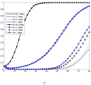
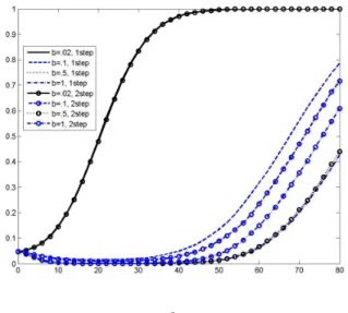
For non-zero values of c we can use the results of Proposition 2 to compute local asymptotic power (LAP) of the modified statistics. Because the limits in Proposition 2 depend on the kernel, bandwidth and form of detrending, we can use LAP to make predictions about the impact of kernel, bandwidth and detrending choices on finite sample power. We simulate LAP for the same set of five kernels and a selection of values ofb. The simulations are performed using partial sums of 1,000

3AlsoMATLABcode to compute the modified test statistics as well as to perform inference using the fixed-b critical values is available from the authors upon request.

8

i.i.d. N(0,1) random errors to approximate the Wiener process that drives the limits in Proposition 2 and 10,000 replications. Local asymptotic power is computed for a grid over c running from 0 to 80 with steps of size 2. Rejections are computed using thec= 0 asymptotic critical value for a given kernel, bandwidth, detrending combination.

We report results for the Bartlett and QS kernels. Results for the other kernels are qualitatively similar. Figures 1-4 plot LAP for the intercept only model whereas Figures 5-8 plot LAP for the intercept and linear trend model. The first notable pattern in these figures is the sensitivity of power to the choice of b. In many cases power decreases asbincreases, but in other cases power is non-monotonic inb. For example, in the intercept and linear trend model,Z_t^m using theQS kernel has good power when b = 0.02, but power drops very quickly when b is increased to 0.1. Then, as b is increased further, power increases but stays well below power when b = 0.02. The second notable pattern is that, except for b = 0.02, there are clear differences in power between the one and two-step detrending approaches with the greatest differences occurring for larger values of b.

The third notable pattern is that power is often very low, often close to zero, when b is not small and c takes on small to medium values. The fourth notable pattern is that the kernel matters for power unless b = 0.02 in which case power is similar for both kernels in all cases. Finally, there are substantial differences in power between theZ_α^m and Z_t^m statistics except when b= 0.02. The local asymptotic power analysis suggests that small bandwidths are much preferable to non-small bandwidths.

4 Finite Sample Behavior

For the sake of brevity we only include a small selection of finite sample results obtained by performing extensive simulations. In particular we only report some results for the sample size T = 200 for the QS kernel for the t-statistic tests. Qualitatively similar results are available also for the coefficient tests, sample size T = 100 and the Bartlett kernel. The number of replications is 5,000 for each experiment. The selected results, for a narrow set of statistics and nuisance parameters, are meant to be illustrative in capturing the main observations in relation to the finite sample predictions of the asymptotic theory. In particular, the fixed-b theory suggests that under the unit root null hypothesis: i) the traditional PP unit root tests will be sensitive to nuisance parameters and the choice of kernel and bandwidth,ii)the modified PP tests will be more robust to nuisance parameters and will be robust to the choice of kernel and bandwidth when the asymptotic fixed-b critical value is used, and iii) there can be a difference between the one- and two-step detrending approaches.

The data generating process is given by (1) and (2) where we setθ=0without loss of generality.

We generate data foru_taccording to theARM A(1,1) model: u_t=ρut−1+ε_t+ϕεt−1 whereε_tis a sequence of i.i.d. N(0,1) random variables fort= 0,1, ..., T andu0= 0.The standard PP test uses

9

the usual unit root asymptotic distribution critical values and is labeled P P. The modified PP test, labeled P P(f b), uses the fixed-b asymptotic critical values corresponding to the limits given in Proposition 2 for c= 0.

In Figures 9–16 we display the empirical null rejection probabilities at the 5% nominal level.

The results are reported for a grid of bandwidths given byM = 2,4,6, . . . ,198,200, indexed by the corresponding value ofb=M/200, with this grid corresponding to the grid for which fixed-bcritical values are available. In all of these figures except for Figure 9 (only intercept) an intercept and a linear time trend are included. In each figure, the rejections are reported for both the one- and two-step detrending. Figures 9 and 10 give results for the case where u_t has no serial correlation (ρ = 0, ϕ = 0). Figure 9 gives results for the intercept case and Figure 10 gives results for the intercept and linear trend case. Several patterns stand out in the figures. The rejections of the P P(f b) tests are close to 0.05 regardless of the bandwidth which indicates that the fixed-bcritical values are doing an adequate job of capturing the dependence of the finite sample distribution on the bandwidth. In contrast, unless a small bandwidth is used, the P P tests have rejections that are not close to 0.05 and the rejections show a sensitivity to the bandwidth. This is consistent with the predictions of Proposition 1. Comparing the one-step with two-step approaches, we see that for the P P tests, there are stark differences in rejection probabilities between the two approaches as predicted by Proposition 1. In contrast, theP P(f b) tests have similar rejections for both one-step and two-step detrending, which is consistent with the fact that the fixed-b limits of the P P(f b) statistics depend on whether one-step or two-step detrending is used.

Figures 11 and 12 give results for MA errors withϕ= 0.4,−0.4. Rejections of theP P statistics are systematically different from 0.05 regardless of the bandwidth. This is consistent with the dependence on serial correlation nuisance parameters indicated by the fixed-b limits of the P P tests. There is a noticeable difference between the one-step and two-step approaches, especially when ϕ = 0.4. The rejections of the P P statistics are even more distorted in the ϕ= −0.4 case and substantial over-rejections are possible for some bandwidths. The rejections of the P P(f b) statistics are very different. When ϕ = 0.4, rejections are close to 0.05 regardless of bandwidth.

In contrast, when ϕ = −0.4, rejections are inflated above 0.05 for the P P(f b) statistics. This general tendency to over-reject when there is a negative MA component is well documented in the literature, see Perron and Ng (1996).

Figures 13 and 14 give results for AR errors withρ= 0.4,−0.4. Similar patterns hold as in the MA case with patterns in theρ = 0.4 case being very similar to the ϕ= 0.4 case and likewise for the ρ = −0.4 and ϕ = −0.4 cases. Intuitively, as either ρ or ϕ approach -1, the spectral density at frequency zero of u_t approaches zero and this counteracts the unit root in y⁰_t leading to over- rejections. Figures 15 and 16 give some results for ARMA errors. When bothρ andϕare positive, rejections of the P P(f b) statistics are close to 0.05 regardless of bandwidth whereas rejections of

10

the P P statistics are highly distorted. When both ρ and ϕ are negative⁴, all statistics tend to over-reject substantially.

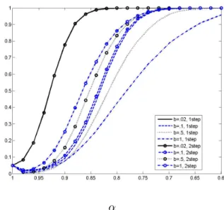
We now turn to some limited finite sample power results to assess the adequacy of the LAP results for theP P(f b) statistics. We only report results forρ= 0,ϕ= 0 and power is size adjusted in all cases. Figure 17 depicts power of the Z_α^m statistics and Figure 18 depicts power for the Z_t^m statistics for the intercept only model. Figures 19 and 20 give results for the intercept and linear trend model. We use the same values of b as for the LAP results. The general patterns in Figures 17-20 are similar to the LAP results. Power is highest for b = 0.02 and power can be much lower for other values of b. There are noticeable differences in power between the one- and two-step approaches and there are also clear differences in power between theZ_α^mandZ_t^mstatistics.

The one notable difference between the LAP power curves and finite sample power curves is that power with T = 200 is generally higher than what is predicted by the LAP analysis. The values of α = 0.9,0.8,0.7,0.6 with T = 200 correspond to values of c = 20,40,60,80. Comparing Figure 8 with Figure 20, notice that power withc= 40 is very low in Figure 8 (except forb= 0.02) whereas power with α = 0.8 is much higher in Figure 20. While the LAP analysis adequately captures the general patterns of power with respect to dependency on bandwidth, model, one- and two-step detrending, etc., the accuracy of the magnitudes of power predicted by the LAP analysis is not so impressive.

5 Summary and Conclusions

The fixed-btheory developed in this paper provides an alternative theoretical explanation for the finite sample dependence of the traditional PP unit root tests on serial correlation in the errors driving the unit root. Unlike the traditional consistency approximation for the long run variance estimators used in the PP tests, the fixed-btheory also indicates a finite sample difference between one-step and two-step detrending. Both local asymptotic power simulations as well as finite sample simulations show that there can be large differences between the one-step and two-step approaches in terms of both null rejection probabilities and power. We propose modified PP statistics that have asymptotically pivotal fixed-b limits. The fixed-b limits depend on the kernel and bandwidth used for the long run variance estimators and the fixed-blimits are different for the one-step and two-step approaches. In finite samples, the modified PP statistics, when used with fixed-b critical values, have null rejections close to the nominal level unless the serial correlation in the innovations to the unit root process behave similarly to an over-differenced stationary process. While the modified PP tests are a clear improvement over the traditional PP tests, further modifications would probably be necessary to make them reliable in practice in terms of adequate size control.

4We do not report results whereρandϕare equal with opposite signs. In this case, the AR and MA components cancel makingut uncorrelated and patterns are essentially identical to those depicted in Figure 10.

11

6 Appendix: Proofs Proof of Lemma 1

With both methods of detrending, the residuals can be written as ub_t,i =ye_t,i−αyet−1,i−T(αb_i−α)yet−1

T ,

with differences occurring asymptotically only in the first part yet,i−αeyt−1,i. We first consider one-step detrending, in which case we obtain

eyt,1−αyet−1,1=eut=ut−D_t⁰(D⁰_TDT)⁻¹D⁰_TUT. This implies that T^−1/2P[rT]

t=2ye_t,1−αyet−1,1 ⇒ ωcW(r)dr. Under the assumptions stated it is well known that T(αb₁ −α) ⇒

ω²R1

0 Vec(s)dW(s)+λ ω²R1

0 Vec(s)²dr

and thatT^−3/2P[rT]

t=2yet−1,1 ⇒ ωRr

0 Ve_c(s)ds. Com- bining these three results establishes (11).

Let us now look at two-step detrending. In this case we can write ye_t,2−αeyt−1,2 =y_t−D⁰_tθb−α(yt−1−D_t−1⁰ θ)b

=y_t⁰+D_t⁰θ−D_t⁰bθ−α(y⁰_t−1+D⁰_t−1θ−D⁰_t−1θ)b

=y_t⁰−αy_t−1⁰ −D_t⁰(θb−θ) +αD⁰_t−1(θb−θ)

=ut−D_t⁰(θb−θ) + (1−cT⁻¹)D⁰_t−1(θb−θ)

=ut−(Dt−Dt−1)⁰(θb−θ)−cT⁻¹D⁰_t−1(θb−θ)

=ut−(Dt−Dt−1)⁰(D_T⁰ DT)⁻¹D⁰_TY_T⁰−cT⁻¹D_t−1⁰ (D⁰_TDT)⁻¹D⁰_TY_T⁰

with Y_T⁰ = [y⁰₂, . . . , y⁰_T]⁰. Defining G_D = diag(1, T, . . . , T^q), straightforward calculations give the standard results

T^−1/2G_D(D⁰_TD_T)⁻¹D_T⁰ Y_T⁰ = (T⁻¹G⁻¹_D D⁰_TD_TG⁻¹_D )⁻¹T^−3/2G⁻¹_D D_T⁰ Y_T⁰

⇒ω Z 1

0

D(s)D(s)⁰ds

⁻¹Z 1 0

D(s)V_c(s)ds, and

T⁻¹

[rT]

X

t=2

D⁰_t−1G⁻¹_D ⇒ Z r

0

D(s)⁰ds.

Less standard, but straightforward, is the result

[rT]

X

t=2

(D_t−Dt−1)⁰G⁻¹_D ⇒ Z r

0

D(s)˙ ⁰ds.

Using these limits and (3), it easily follows thatT^−1/2P[rT]

t=2(yet,2−αyet−1,2)⇒ωVe˙c(r). Combining this result with the unchanged results (compared to the one-step detrending) for the other two components establishes (12).

12

Proof of Proposition 1

The results of the proposition follow from the asymptotic result for the partial sum processes of the residuals established in Lemma 1, using similar arguments as in Hashimzade and Vogelsang (2008).

Once the fixed-b limits for ωb²_i, i∈ {1,2} are established, the fixed-b limit distributions of the test statistics follow from using these when calculating the limiting distributions of the test statistics, as given in (9) and (10), with these expressions referring to one-step detrending and the two-step detrending versions of the test statistics similarly defined.

Proof of Lemma 2

The proof of the lemma builds heavily on the proof of Lemma 1, with in fact only the term comprisingαbi being different in the expressions for the modified residuals compared to the residuals previously considered. For both detrending approaches it holds that

T(αb^m_i −α) =T(αb_i−α) +

1 2bσ_i² T⁻²PT

t=2ye_t−1,i²

⇒ ω²R1

0 Vec(r)dW(r) +λ ω²R1

0 Ve_c(r)²dr +

1 2σ² ω²R1

0 Ve_c(r)²dr

= R₁

0 Vec(r)dW(r) +¹₂ R1

0 Ve_c(r)²dr ,

from which the results of the lemma follow, since all other terms are unchanged compared to Lemma 1.

Proof of Proposition 2

Using the result from Lemma 2 the limit ofZ_α,i^∗ follows immediately:

T(αb^m_i −1) =T(αb^m_i −α+α−1) =T(αb^m_i −α) +T(α−1)

=T(αb^m_i −α)−c

⇒ −c+ R1

0 Ve_c(r)dW(r) +¹₂ R1

0 Ve_c(r)²dr .

The other results follow, similar to the results of Proposition 1, from the asymptotic result for the partial sum processes of the modified residuals established in Lemma 2 using now the fixed-blimit for the modified long run variance estimatorsωe_i² in place of ωb_i².

13

References

Hashimzade, N. and T.J. Vogelsang (2008). Fixed-b Asymptotic Approximation of the Sampling Behavior of Nonparametric Spectral Density Estimators. Journal of Time Series Analysis 29, 142–162.

Jansson, M. (2002). Consistent Covariance Matrix Estimation for Linear Processes. Econometric Theory 18, 1449–1459.

Kiefer, N.M. and T.J. Vogelsang (2005). A New Asymptotic Theory for Heteroskedasticity- Autocorrelation Robust Tests. Econometric Theory 21, 1130–1164.

Perron, P. and S. Ng (1996). Useful Modifications to some Unit Root Tests with Dependent Errors and their Local Asymptotic Properties.Review of Economic Studies 63, 435–463.

Perron, P. and T.J. Vogelsang (1992). Testing for a Unit Root in a Time Series with a Changing Mean: Corrections and Extensions. Journal of Business and Economic Statistics 10, 467–470.

Phillips, P.C.B. (1987). Towards a Unified Asymptotic Theory for Autoregression.Biometrika 74, 535–547.

Phillips, P.C.B. and P. Perron (1988). Testing for a Unit Root in Time Series Regression.Biometrika 75, 335–346.

Phillips, P.C.B and V. Solo (1992). Asymptotics for Linear Processes.The Annals of Statistics 20, 971–1001.

Schwert, W. (1989). Tests for Unit Roots: A Monte Carlo Investigation.Journal of Business and Economic Statistics 7, 147–159.

Sims, C.A., J.H. Stock and M.W. Watson (1990). Inference in Linear Time Series Models with some Unit Roots. Econometrica 58, 113-144.

14

c c

Figure 1: Local Asymptotic Power, Z_α^m, Bartlett Figure 2: Local Asymptotic Power,Z_t^m, Bartlett

Intercept Only Intercept Only

c c

Figure 3: Local Asymptotic Power,Z_α^m, QS Figure 4: Local Asymptotic Power, Z_t^m, QS

Intercept Only Intercept Only

15

c c

Figure 5: Local Asymptotic Power, Z_α^m, Bartlett Figure 6: Local Asymptotic Power,Z_t^m, Bartlett

Intercept+Linear Trend Intercept+Linear Trend

c c

Figure 7: Local Asymptotic Power,Z_α^m, QS Figure 8: Local Asymptotic Power, Z_t^m, QS

Intercept+Linear Trend Intercept+Linear Trend

16

b b

Figure 9: Empirical Null Rejections, Z_t^m, QS Figure 10: Empirical Null Rejections,Z_t^m, QS Intercept Only, ρ= 0,ϕ= 0 Intercept+Linear Trend, ρ= 0, ϕ= 0

b b

Figure 11: Empirical Null Rejections,Z_t^m, QS Figure 12: Empirical Null Rejections,Z_t^m, QS Intercept+Linear Trend, ρ= 0,ϕ= 0.4 Intercept+Linear Trend,ρ= 0, ϕ=−0.4

17

b b

Figure 13: Empirical Null Rejections,Z_t^m, QS Figure 14: Empirical Null Rejections,Z_t^m, QS Inter.+Lin. Trend, ρ= 0.4, ϕ= 0,T = 200 Inter.+ Lin. Trend, ρ=−0.4, ϕ= 0,T = 200

b b

Figure 15: Empirical Null Rejections,Z_t^m, QS Figure 16: Empirical Null Rejections,Z_t^m, QS Inter.+Lin. Trend, ρ= 0.4,ϕ= 0.4, T = 200 Inter.+Lin. Trend, ρ=−0.4,ϕ=−0.4,T = 200

18

α α

Figure 17: Finite Sample Power (size adjusted) Figure 18: Finite Sample Power (size adjusted) Z_α^m, QS, Intercept Only, ρ= 0,ϕ= 0, T = 200 Z_t^m, QS, Intercept Only, ρ= 0,ϕ= 0, T = 200

α α

Figure 19: Finite Sample Power (size adjusted) Figure 20: Finite Sample Power (size adjusted) Z_α^m, QS, Inter.+Lin. Trend, ρ= 0,ϕ= 0, T = 200 Z_t^m, QS, Inter.+Lin. Trend, ρ= 0,ϕ= 0, T = 200

19

Authors: Timothy J. Vogelsang, Martin Wagner

Title: A Fixed-b Perspective on the Phillips-Perron Unit Root Tests Reihe Ökonomie / Economics Series 272

Editor: Robert M. Kunst (Econometrics)

Associate Editors: Walter Fisher (Macroeconomics), Klaus Ritzberger (Microeconomics)

ISSN: 1605-7996

© 2011 by the Department of Economics and Finance, Institute for Advanced Studies (IHS),

Stumpergasse 56, A-1060 Vienna   +43 1 59991-0  Fax +43 1 59991-555  http://www.ihs.ac.at

ISSN: 1605-7996