SFB 823
Two-sample tests for relevant differences in the
eigenfunctions of covariance operators
Discussion Paper Alexander Aue, Holger Dette, Gregory Rice
Nr. 22/2019
Two-sample tests for relevant differences in the eigenfunctions of covariance operators
Alexander Aue∗ Holger Dette† Gregory Rice‡ September 11, 2019
Abstract
This paper deals with two-sample tests for functional time series data, which have become widely available in conjunction with the advent of modern complex observation systems. Here, particular interest is in evaluating whether two sets of functional time series observations share the shape of their primary modes of variation as encoded by the eigenfunctions of the respective covariance operators. To this end, a novel testing approach is introduced that connects with, and extends, existing literature in two main ways. First, tests are set up in the relevant testing framework, where interest is not in testing an exact null hypothesis but rather in detecting deviations deemed sufficiently relevant, with relevance determined by the practitioner and perhaps guided by domain experts. Second, the proposed test statistics rely on a self-normalization principle that helps to avoid the notoriously difficult task of estimating the long-run covariance structure of the underlying functional time series. The main theoretical result of this paper is the derivation of the large-sample behavior of the proposed test statistics. Empirical evidence, indicating that the proposed procedures work well in finite samples and compare favorably with competing methods, is provided through a simulation study, and an application to annual temperature data.
Keywords:Functional data; Functional time series; Relevant tests; Self-normalization; Two-sample tests.
1 Introduction
This paper develops testing tools for two independent sets of functional observations, explicitly allowing for temporal dependence within each set. Functional data analysis has become a mainstay for dealing with those complex data sets that may conceptually be viewed as being comprised of curves. Monographs detailing many of the available statistical procedures for functional data are Ramsay and Silverman (2005) and Horv´ath and Kokoszka (2012). This type of data naturally arises in various contexts such as environmental data (Aue et al., 2015), molecular biophysics (Tavakoli and Panaretos, 2016), climate science (Zhang et al., 2011; Aue et al., 2018a), and economics (Kowal et al., 2019). Most of these examples intrinsically contain a time series
∗Department of Statistics, University of California, One Shields Avenue, Davis, CA 95616, USA, email:aaue@ucdavis.edu
†Fakult¨at f¨ur Mathematik, Ruhr-Universit¨at Bochum, Bochum, Germany, email:holger.dette@rub.de
‡Department of Statistics and Actuarial Science, University of Waterloo, Waterloo, ON, Canada, email:
grice@uwaterloo.ca
component as successive curves are expected to depend on each other. Because of this, the literature on functional time series has grown steadily; see, for example, H¨ormann and Kokoszka (2010), Panaretos and Tavakoli (2013) and the references therein.
The main goal here is towards developing two-sample tests for comparing the second order properties of func- tional time series data. Two-sample inference and testing methods for curves have been developed extensively by several authors. Hall and Van Keilegom (2007) were concerned with the effect of pre-processing discrete data into functions on two-sample testing procedures. Horv´ath et al. (2013) investigated two-sample tests for the equality of means of two functional time series taking values in the Hilbert space of square integrable functions, and Dette et al. (2019) introduced multiplier bootstrap-assisted two-sample tests for functional time series taking values in the Banach space of continuous functions. Panaretos et al. (2010), Fremdt et al. (2013), Pigoli et al. (2014), Paparoditis and Sapatinas (2016) and Guo et al. (2016) provided procedures for testing the equality of covariance operators in functional samples.
While general differences between covariance operators can be attributed to differences in the eigenfunctions of the operators, eigenvalues of the operators, or perhaps both, we focus here on constructing two sample tests that take aim only at differences in the eigenfunctions. The eigenfunctions of covariance operators hold a special place in functional data analysis due to their near ubiquitous use in dimension reduction via functional principal component analysis (FPCA). FPCA is the basis of the majority of inferential procedures for functional data. In fact, an assumption common to a number of such procedures is that observations from different samples/populations share a common eigenbasis generated by their covariance operators; see Benko et al. (2009) and Pomann et al. (2016). FPCA is arguably even more crucial to the analysis of functional time series, since it underlies most forecasting and change-point methods, see e.g. Aue et al. (2015), Hyndman and Shang (2009), and Aston and Kirch (2012). The tests proposed here are useful both for determining the plausibility that two samples share similar eigenfunctions, or whether or not one should pool together data observed in different samples for a joint analysis of their principal components. We illustrate these applications in Section 4 below in an analysis of annual temperature profiles recorded at several locations, for which the shape of the eigenfunctions can help in the interpretation of geographical differences in the primary modes of temperature variation over time. A more detailed argument for the usefulness and impact of such tests on validating climate models is given in the introduction of Zhang and Shao (2015), to which the interested reader is referred to for details.
The procedures introduced in this paper are noteworthy in at least two respects. First, unlike existing literature, they are phrased in the relevant testing framework. In this paradigm, deviations from the null are deemed of interest only if they surpass a minimum threshold set by the practitioner. Classical hypothesis tests are included in this approach if the threshold is chosen to be equal to zero. There are several advantages coming with the relevant framework. In general, it avoids Berkson’s consistency problem (Berkson, 1938) that any consistent test will reject for arbitrarily small differences if the sample size is large enough. More specific to functional data, theL2-norm sample mean curve differences might not be close to zero even if the underlying population
mean curves coincide. The adoption of the relevant framework typically comes at the cost of having to invoke involved theoretical arguments. A recent review of methods for testing relevant hypotheses in two sample problems with one-dimensional data from a biostatistics perspective can be found in Wellek (2010), while Section 2 specifies the details important here.
Second, the proposed two-sample tests are built using self-normalization, a recent concept for studentizing test statistics introduced originally for univariate time series in Shao (2010) and Shao and Zhang (2010). When conducting inference with time series data, one frequently encounters the problem of having to estimate the long-run variance in order to scale the fluctuations of test statistics. This is typically done through estimators relying on tuning parameters that ideally should adjust to the strength of the autocorrelation present in the data. In practice, the success of such methods can vary widely. As a remedy, self-normalization is a tuning parameter-free method that achieves standardization, typically through recursive estimates. The advantages of such an approach for testing relevant hypotheses of parameters of functional time series were recently recog- nized in Dette et al. (2018). In this paper, we develop a concept of self-normalization for the problem of testing for relevant differences between the eigenfunctions of two covariance operators in functional data. Zhang and Shao (2015) is the work most closely related to the results presented below, as it pertains to self-normalized two-sample tests for eigenfunctions and eigenvalues in functional time series. An important difference to this work is that the methods proposed here do not require a dimension reduction of the eigenfunctions but com- pare the functions directly with respect to a norm in the L2-space. A further crucial difference is that their paper is in the classical testing setup, while ours is in the strictly relevant setting, so that the contributions are not directly comparable on the same footing—even though we report the outcomes from both tests on the same simulated curves in Section 3. There, it is found that, despite the fact that the proposed test is constructed to detect relevant differences, it appears to compare favorably against the test of Zhang and Shao (2015) when the difference in eigenfunctions is large. In this sense, both tests can be seen as complementing each other.
The rest of the paper is organized as follows. Section 2 introduces the framework, details model assumptions and gives the two-sample test procedures as well as their theoretical properties. Section 3 reports the results of a comparative simulation study. Section 4 showcases an application of the proposed tests to Australian temperature curves obtained at different locations during the past century or so. Section 5 concludes. Finally some technical details used in the arguments of Section 2.2 are given in Section 6.
2 Testing the similarity of two eigenfunctions
Let L2([0,1]) denote the common space of square integrable functions f: [0,1] → R with inner product hf1, f2i=R1
0 f1(t)f2(t)dtand normkfk= R1
0 f2(t)dt1/2
. Consider two independent stationary functional time series(Xt)t∈Zand(Yt)t∈ZinL2([0,1])and assume that eachXtandYtis centered and square integrable, that isE[Xt] = 0,E[Yt] = 0andE[kXtk2]< ∞,E[kYtk2]<∞, respectively. In practice centering can be
achieved by subtracting the sample mean function estimate and this will not change our results. Denote by CX(s, t) =
∞
X
j=1
τjXvXj (s)vXj (t), (2.1)
CY(s, t) =
∞
X
j=1
τjYvjY(s)vjY(t) (2.2)
the corresponding covariance operators; see Section 2.1 of B¨ucher et al. (2019) for a detailed discussion of expected values in Hilbert spaces. The eigenfunctions of the kernel integral operators with kernelsCX andCY, corresponding to the ordered eigenvaluesτ1X ≥ τ2X ≥ · · · andτ1Y ≥ τ2Y ≥ · · ·, are denoted by v1X, vX2 , . . .andv1Y, v2Y, . . ., respectively. We are interested in testing the similarity of the covariance operators CX andCY by comparing their eigenfunctionsvjX andvYj of orderjfor somej ∈N. This is framed as the relevant hypothesis testing problem
H0(j):kvjX −vYj k2≤∆j versus H1(j):kvjX −vjYk2>∆j, (2.3) where∆j > 0is a pre-specified constant representing the maximal value for the squared distanceskvjX − vjYk2 between the eigenfunctions which can be accepted as scientifically insignificant. In order to make the comparison between the eigenfunctions meaningful, we assume throughout this paper thathvjX, vjYi ≥ 0for allj∈N. The choice of the threshold∆j >0depends on the specific application and is essentially defined by the change size one is really interested in from a scientific viewpoint. In particular, the choice∆j = 0gives the classical hypothesesH0c:vXj =vjY versusH1c:vXj 6=vjY. We argue, however, that often it is well known that the eigenfunctions, or other parameters for that matter, from different samples will not precisely coincide.
Further there is frequently no actual interest in arbitrarily small differences between the eigenfunctions. For this reason,∆j >0is assumed throughout.
Observe also that a similar hypothesis testing problem could be formulated for relevant differences of the eigenvaluesτjX −τjY of the covariance operators. We studied the development of such tests alongside those presented below for the eigenfunctions, and found, interestingly, that they generally are less powerful empiri- cally. An elaboration and explanation of this is detailed in Remark 2.1 below. The arguments presented there are also applicable to tests based on direct long-run variance estimation.
The proposed approach is based on an appropriate estimate, sayDˆ(j)m,n, of the squaredL2-distancekvjX−vYj k2 between the eigenfunctions, and the null hypothesis in (2.3) is rejected for large values of this estimate. It turns out that the (asymptotic) distribution of this distance depends sensitively on all eigenvalues and eigenfunctions of the covariance operatorsCX andCY and on the dependence structure of the underlying processes. To address this problem we propose a self-normalization of the statistic Dˆm,n(j) . Self-normalization is a well- established concept in the time series literature and was introduced in two seminal papers by Shao (2010) and Shao and Zhang (2010) for the construction of confidence intervals and change point analysis, respectively.
More recently, it has been developed further for the specific needs of functional data by Zhang et al. (2011) and Zhang and Shao (2015); see also Shao (2015) for a recent review on self-normalization. In the present
context, where one is interested in hypotheses of the form (2.3), a non-standard approach of self-normalization is necessary to obtain a distribution-free test, which is technically demanding due to the implicit definition of the eigenvalues and eigenfunctions of the covariance operators. For this reason, we first present the main idea of our approach in Section 2.1 and defer a detailed discussion to the subsequent Section 2.2.
2.1 Testing for relevant differences between eigenfunctions
IfX1, . . . , XmandY1, . . . , Ynare the two samples, then CˆmX(s, t) = 1
m
m
X
i=1
Xi(s)Xi(t), CˆnY(s, t) = 1 n
n
X
i=1
Yi(s)Yi(t) (2.4)
are the common estimates of the covariance operators (Ramsay and Silverman, 2005; Horv´ath and Kokoszka, 2012). Denote by τˆjX,ˆτjY and vˆXj ,ˆvYj the corresponding eigenvalues and eigenfunctions. Together, these define the canonical estimates of the respective population quantities in (2.1) and (2.2). Again, to make the comparison between the eigenfunctions meaningful, it is assumed throughout this paper that the inner product ofhˆvjX,vˆjYi is nonnegative for allj, which can be achieved in practice by changing the sign of one of the eigenfunction estimates if needed. We use the statistic
Dˆm,n(j) =kˆvjX −vˆjYk2= Z 1
0
(ˆvjX(t)−ˆvYj (t))2dt (2.5) to estimate the squared distance
D(j)=kvjX −vYj k2= Z 1
0
(vjX(t)−vjY(t))2dt (2.6) between the jth population eigenfunctions. The null hypothesis will be rejected for large values of Dˆm,n(j)
compared to ∆j. In the following, a self-normalized test statistic based on Dˆ(j)m,n will be constructed; see Dette et al. (2018). To be precise, letλ∈[0,1]and define
CˆmX(s, t, λ) = 1 bmλc
bmλc
X
i=1
Xi(s)Xi(t), CˆnY(s, t, λ) = 1 bnλc
bnλc
X
i=1
Yi(s)Yi(t) (2.7) as the sequential version of the estimators in (2.4), noting that the sums are defined as 0 if bmλc < 1.
Observe that, under suitable assumptions detailed in Section 2.2, the statistics CˆmX(·,·, λ) and CˆnY(·,·, λ) are consistent estimates of the covariance operators CX andCY, respectively, whenever0 < λ ≤ 1. The corresponding sample eigenfunctions of CˆmX(·,·, λ) and CˆnY(·,·, λ) are denoted by vˆjX(t, λ) andvˆjY(t, λ), respectively, assuming throughout thathˆvjX,vˆjYi ≥0. Define the stochastic process
Dˆ(j)m,n(t, λ) =λ(ˆvjX(t, λ)−vˆjY(t, λ)), t∈[0,1], λ∈[0,1], (2.8) and note that the statisticDˆm,n(j) in (2.5) can be represented as
Dˆ(j)m,n = Z 1
0
( ˆDm,n(j) (t,1))2dt. (2.9)
Self-normalization is enabled through the statistic Vˆm,n(j) =Z 1
0
Z 1
0
( ˆD(j)m,n(t, λ))2dt−λ2 Z 1
0
( ˆDm,n(j) (t,1))2dt2
ν(dλ)1/2
, (2.10)
whereν is a probability measure on the interval(0,1]. Note that, under appropriate assumptions, the statistic Vˆm,n(j) converges to0in probability. However, it can be proved that its scaled version√
m+nVˆm,n(j) converges in distribution to a random variable, which is positive with probability 1. More precisely, it is shown in Theorem 2.2 below that, under an appropriate set of assumptions,
√m+n Dˆ(j)m,n−D(j),Vˆm,n(j) D
−→
ζjB(1), n
ζj2 Z 1
0
λ2(B(λ)−λB(1))2ν(dλ) o1/2
(2.11) asm, n→ ∞, whereD(j)is defined in (2.6). Here{B(λ)}λ∈[0,1]is a Brownian motion on the interval[0,1]
andζj ≥0is a constant, which is assumed to be strictly positive ifDj >0(the squareζj2is akin to a long-run variance parameter). Consider then the test statistic
Wˆ(j)m,n := Dˆ(j)m,n−∆j
Vˆm,n(j)
. (2.12)
Based on this, the null hypothesis in (2.3) is rejected whenever
Wˆ(j)m,n > q1−α, (2.13)
whereq1−αis the(1−α)-quantile of the distribution of the random variable W:= B(1)
{R1
0 λ2(B(λ)−λB(1))2ν(dλ)}1/2. (2.14) The quantiles of this distribution do not depend on the long-run variance, but on the measureνin the statistic Vˆm,n(j) used for self-normalization. An approximateP-value of the test can be calculated as
p=P(W>Wˆ(j)m,n). (2.15)
The following theorem shows that the test just constructed keeps a desired level in large samples and has power increasing to one with the sample sizes.
Theorem 2.1. If the weak convergence in (2.11) holds, then the test(2.13) has asymptotic level α and is consistent for the relevant hypotheses in(2.3). In particular,
m,n→∞lim P( ˆW(j)m,n > q1−α) =
0 if D(j)<∆j. α if D(j)= ∆j. 1 if D(j)>∆j.
(2.16) 2
Proof. IfDj >0, the continuous mapping theorem and (2.11) imply Dˆ(j)m,n−D(j)
Vˆm,n(j)
−→D W, (2.17)
where the random variableWis defined in (2.14). Consequently, the probability of rejecting the null hypoth- esis is given by
P( ˆW(j)m,n > q1−α) =P
Dˆ(j)m,n−D(j) Vˆm,n(j)
> ∆j−D(j) Vˆm,n(j)
+q1−α
. (2.18)
It follows moreover from (2.11) that Vˆm,n(j) →P 0 as m, n → ∞ and therefore (2.17) implies (2.16), thus completing the proof in the caseDj >0. IfDj = 0it follows from the proof of (2.11) (see Proposition 2.2 below) that√
m+nDˆm,n(j) =oP(1)and√
m+nVˆm,n(j) =oP(1). Consequently, P( ˆW(j)m,n > q1−α) =P
√m+nDˆm,n(j) >√
m+n∆j+√
m+nVˆm,n(j)q1−α
=o(1),
which completes the proof.
The main difficulty in the proof of Theorem 2.1 is hidden by postulating the weak convergence in (2.11). A proof of this statement is technically demanding. The precise formulation is given in the following section.
Remark 2.1(Estimation of the long-run variance, power, and relevant differences in the eigenvalues).
(1) The parameterζj2 is essentially a long-run variance parameter. Therefore it is worthwhile to mention that on a first glance the weak convergence in (2.11) provides a very simple test for the hypotheses (2.3) if a consistent estimator, sayζˆn,j2 , of the long-run variance would be available. To this end, note that in this case it follows from (2.11) that√
m+n( ˆD(j)m,n−D(j))/ζˆn,j converges weakly to a standard normal distribution.
Consequently, using the same arguments as in the proof of Theorem 2.1,we obtain that rejecting the null hypothesis in (2.3), whenever
√m+n( ˆDm,n(j) −∆j)/ζˆn,j > u1−α, (2.19) yields a consistent and asymptotic level α test. However a careful inspection of the representation of the long-run variance in equations (6.11)–(6.15) in Section 6 suggests that it would be extremely difficult, if not impossible, to construct a reliable estimate of the parameterζj in this context, due to its complicated depen- dence on the covariance operatorsCX,CY, and their full complement of eigenvalues and eigenfunctions.
(2) DefiningK= R1
0 λ2(B(λ)−λB(1))2ν(dλ)1/2
, it follows from (2.18) that P Wˆ(j)m,n > q1−α
≈P
W>
√m+n(∆j−Dj)
ζj·K +q1−α
, (2.20)
where the random variable W is defined in (2.14) and ζj is the long-run standard deviation appearing in Theorem 2.2, which is defined precisely in (6.15). The probability on the right-hand side converges to zero,α, or 1, depending on∆j−Dj being negative, zero, or positive, respectively. From this one may also quite easily
understand how the power of the test depends onζj. Under the alternative,∆j −Dj <0and the probability on the right-hand side of (2.20) increases if(Dj−∆j)/ζjincreases. Consequently, smaller long-run variances ζj2 yield more powerful tests. Some values ofζj are calculated via simulation for some of the examples in Section 3 below.
(3) Alongside the test for relevant differences in the eigenfunctions just developed, one might also consider the following test for relevant differences in thejth eigenvalues of the covariance operatorsCX andCY:
H0,val(j) : Dj,val := (τjX −τjY)2 ≤∆j,val versus H1,val(j) : (τjX −τjY)2 >∆j,val. (2.21) Following the development of the above test for the eigenfunctions, a test of the hypothesis (2.21) can be constructed based on the partial sample estimates of the eigenvaluesˆτjX(λ)andτˆjY(λ)of the kernel integral operators with kernelsCˆmX(·,·, λ)andCˆnY(·,·, λ)in (2.7). In particular, let
Tˆm,n(j) (λ) = λ(ˆτjX(λ)−τˆjY(λ)), and Mˆm,n(j) =
Z 1 0
{[ ˆTm,n(j)(λ)]2−λ2[ ˆTm,n(j)(λ)]2}2ν(dλ) 1/2
.
Then one can show, in fact somewhat more simply than in the case of the eigenfunctions, that the test procedure that rejects the null hypothesis whenever
Qˆ(j)m,n =
Tˆm,n(j)(1)−∆j,val
Mˆm,n(j) > q1−α (2.22)
is a consistent and asymptotic level α test for the hypotheses (2.21). Moreover, the power of this test is approximately given by
P Qˆ(j)m,n > q1−α
≈P W>
√m+n(∆j,val−Dj,val)
ζj,val·K +q1−α
, (2.23)
whereζj,val2 is a different long-run variance parameter. Although the tests (2.3) and (2.21) are constructed for completely different testing problems it might be of interest to compare their power properties. For this purpose note that the ratios(Dj −∆j)/ζj and(Dj,val−∆j,val)/ζj,val, for which the power of each test is an increasing function of, implicitly depend in a quite complicated way on the dependence structure of theX andY samples and on all eigenvalues and eigenfunctions of their corresponding covariance operators.
One might expect intuitively that relevant differences between the eigenvalues would be easier to detect than differences between the eigenfunctions (as the latter are more difficult to estimate). However, an empirical analysis shows that, in typical examples, the ratio(Dj,val−∆j,val)/ζj,val increases extremely slowly with increasingDj,valcompared to the analogous ratio for the eigenfunction problem. Consequently, we expected and observed in numerical experiments (not presented for the sake of brevity) that the test (2.22) would be less powerful than the test (2.13) if in hypotheses (2.21) and (2.3) the thresholds∆j,val and∆j are similar.
This observation also applies to the tests based on (intractable) long-run variance estimation. Here the power is approximately given by1−Φ √
m+n(∆j −D)/z+u1−α
, whereΦis the cdf of the standard normal distribution andz(andD) is eitherζj (andDj) for the test (2.19) orζj,val(andDj,val) for the corresponding test regarding the eigenvalues.
2.2 Justification of weak convergence
For a proof of (2.11) several technical assumptions are required. The first condition is standard in two-sample inference.
Assumption 2.1. There exists a constantθ∈(0,1)such thatlimm,n→∞m/(m+n) =θ.
Next, we specify the dependence structure of the time series {Xi}i∈Z and {Yi}i∈Z. Several mathematical concepts have been proposed for this purpose (see Bradley, 2005; Bertail et al., 2006, among many others). In this paper, we use the general framework ofLp-m-approximability for weakly dependent functional data as put forward in H¨ormann and Kokoszka (2010). Following these authors, a time series{Xi}i∈ZinL2([0,1]) is calledLp-m-approximablefor somep >0if
(a) There exists a measurable functiong:S∞→ L2([0,1]), whereSis a measurable space, and indepen- dent, identically distributed (iid) innovations{i}i∈Ztaking values inSsuch thatXi =g(i, i−1, . . .) fori∈Z;
(b) Let{0i}i∈Zbe an independent copy of{i}i∈Z, and define Xi,m =g(i, . . . , i−m+1, 0i−m, 0i−m−1, . . .). Then,
∞
X
m=0
E[kXi−Xi,mkp]1/p
<∞.
Assumption 2.2. The sequences{Xi}i∈Zand{Yi}i∈Zare independent, each centered andLp-m-approximable for somep >4.
Under Assumption 2.2, there exist covariance operators CX and CY ofXi andYi. For the corresponding eigenvaluesτ1X ≥τ2X ≥ · · · andτ1Y ≥τ2Y ≥ · · ·, we assume the following.
Assumption 2.3. There exists a positive integerdsuch thatτ1X >· · · > τdX > τd+1X >0andτ1Y > · · · >
τdY > τd+1Y >0.
The final assumption needed is a positivity condition on the long-run variance parameter ζj2 appearing in (2.11). The formal definition ofζjis quite cumbersome, since it depends in a complicated way on expansions for the differencesˆvXj (·, λ)−vXj andˆvYj (·, λ)−vYj , but is provided in Section 6; see equations (6.11)–(6.15).
Assumption 2.4. The scalarζjdefined in(6.15)is strictly positive, wheneverDj >0.
Recall the definition of the sequential processesCˆX(·,·, λ)andCˆY(·,·, λ) in (2.7) and their corresponding eigenfunctionsˆvXj (·, λ)andˆvYj (·, λ). The first step in the proof of the weak convergence (2.11) is a stochas- tic expansion of the difference between the sample eigenfunctionsvˆjX(·, λ)andˆvYj (·, λ)and their respective population versionsvjXandvjY. Similar expansions that do not take into account uniformity in the partial sam- ple parameterλhave been derived by Kokoszka and Reimherr (2013) and Hall and Hosseini-Nasab (2006), among others; see also Dauxois et al. (1982) for a general statement in this context. The proof of this result is postponed to Section 6.1.
Proposition 2.1. Suppose Assumptions 2.2 and 2.3 hold, then, for anyj ≤d, sup
λ∈[0,1]
λ[ˆvXj (t, λ)−vXj (t)]− 1
√m X
k6=j
vXk(t) τjX −τkX
Z 1 0
ZˆmX(s1, s2, λ)vkX(s2)vjX(s1)ds1ds2
(2.24)
=OP
logκ(m) m
,
and sup
λ∈[0,1]
λ[ˆvjY(t, λ)−vYj (t)]− 1
√m X
k6=j
vYk(t) τjY −τkY
Z 1 0
ZˆnY(s1, s2, λ)vkY(s2)vjY(s1)ds1ds2
(2.25)
=OP
logκ(n) n
,
for someκ >0, where the processesZˆmX andZˆnY are defined by
ZˆmX(s1, s2, λ) = 1
√m
bmλc
X
i=1
Xi(s1)Xi(s2)−CX(s1, s2)
, (2.26)
ZˆnY(s1, s2, λ) = 1
√n
bnλc
X
i=1
Yi(s1)Yi(s2)−CY(s1, s2)
. (2.27)
Moreover,
sup
λ∈[0,1]
√ λ
ˆvXj (·, λ)−vjX
=OP log(1/κ)(m)
√m
!
, (2.28)
sup
λ∈[0,1]
√ λ
ˆvYj (·, λ)−vjY
=OP log(1/κ)(n)
√n
!
. (2.29)
Recalling notation (2.8), Proposition 2.1 motivates the approximation
Dˆ(j)m,n(t, λ)−λDj(t) =λ(ˆvjX(t)−ˆvYj (t))−λ(vXj (t)−vjY(t))≈D˜m,n(j) (t, λ), (2.30) where the processD˜(j)m,nis defined by
D˜(j)m,n(t, λ) = 1
√m X
k6=j
vXk(t) τjX −τkX
Z 1 0
ZˆmX(s1, s2, λ)vXk (s2)vjX(s1)ds1ds
− 1
√n X
k6=j
vkY(t) τjY −τkY
Z 1 0
ZˆnY(s1, s2, λ)vYk(s2)vYj (s1)ds1, ds2. (2.31)
The next result makes the foregoing heuristic arguments rigorous and shows that the approximation holds in fact uniformly with respect toλ∈[0,1].
Proposition 2.2. Suppose Assumptions 2.1–2.4 hold, then, for any forj≤d, sup
λ∈[0,1]
Dˆ(j)m,n(·, λ)−λDj(·)−D˜m,n(j) (·, λ) =oP
1
√m+n
,
sup
λ∈[0,1]
Dˆ(j)m,n(·, λ)−λDj(·)
2−
D˜(j)m,n(·, λ)
2
=oP
1
√m+n
,
and √
m+n sup
λ∈[0,1]
Z 1
0
( ˜Dm,n(j) (t, λ))2dt=oP(1). (2.32) Proof. According to their definitions,
Dˆm,n(j) (t, λ)−λDj(t)−D˜(j)m,n(t, λ)
=λ[ˆvXj (t, λ)−vXj (t)]− 1
√m X
k6=j
vXk(t) τjX −τkX
Z 1 0
ZˆmX(s1, s2, λ)vXk (s2)vjX(s1)ds1ds2
+λ[ˆvjY(t, λ)−vjY(t)]− 1
√m X
k6=j
vkY(t) τjY −τkY
Z 1 0
ZˆnY(s1, s2, λ)vkY(s2)vjY(s1)ds1ds2.
Therefore, by the triangle inequality, Proposition 2.1, and Assumption 2.1, sup
λ∈[0,1]
Dˆ(j)m,n(·, λ)−λDj(·)−D˜m,n(j) (·, λ)
≤ sup
λ∈[0,1]
λ[ˆvjX(t, λ)−vjX(t)]− 1
√m X
k6=j
vXk (t) τjX −τkX
Z 1 0
ZˆmX(s1, s2, λ)vkX(s2)vjX(s1)ds1ds2
+ sup
λ∈[0,1]
λ[ˆvjY(t, λ)−vjY(t)]− 1
√m X
k6=j
vkY(t) τjY −τkY
Z 1
0
ZˆnY(s1, s2, λ)vYk(s2)vjY(s1)ds1ds2
=OP
logκ(m) m
=oP 1
√m+n
.
The second assertion follows immediately from the first and the reverse triangle inequality. With the second assertion in place, we have, using (2.28) and (2.29), that
√m+n sup
λ∈[0,1]
Z 1 0
( ˜D(j)m,n(t, λ))2dt=√
m+n sup
λ∈[0,1]
Z 1 0
( ˆD(j)m,n(t, λ)−λDj(t))2dt+oP(1)
≤4√ m+n
h sup
λ∈[0,1]
λ2kˆvjX(·, λ)−vXj k2+ sup
λ∈[0,1]
λ2kˆvjY(·, λ)−vjYk2i
=OP
log(2/κ)(m)
√m
=oP(1) which completes the proof.
Introduce the process
Zˆm,n(j) (λ) =√ m+n
Z 1 0
(( ˆD(j)m,n(t, λ))2−λ2Dj2(t))dt (2.33) to obtain the following result. The proof is somewhat complicated and therefore deferred to Section 6.2.
Proposition 2.3. LetZˆm,n(j) be defined by(2.33), then, under Assumptions 2.1-2.4 we have for anyj ≤d, {Zˆm,n(j) (λ)}λ∈[0,1] {λζjB(λ)}λ∈[0,1],
where ζj is a positive constant, {B(λ)}λ∈[0,1] is a Brownian motion and denotes weak convergence in Skorokhod topology onD[0,1].
Theorem 2.2. If Assumptions 2.1, 2.2 and 2.3 are satisfied, then for anyj≤d
√m+n Dˆm,n(j) −D(j),Vˆm,n(j)
ζjB(1),n ζj2
Z 1 0
λ2(B(λ)−λB(1))2ν(dλ)o1/2 ,
whereDˆ(j)m,nandVˆm,n(j) are defined by(2.9)and(2.10), respectively, and{B(λ)}λ∈[0,1]is a Brownian motion.
Proof. Observing the definition ofDˆm,n(j) ,D(j),Zˆm,n(j) andVˆm,n(j) in (2.9), (2.6) and (2.33) and (2.10), we have Dˆ(j)m,n−D(j) =
Z 1
0
( ˆDm,n(t,1))2dt− Z 1
0
Dj2(t)dt= Zˆm,n(j) (1)
√m+n, Vˆm,n(j) = nZ 1
0
Z 1 0
( ˆDm,n(j) (t, λ))2−λ2Dj2(t) dt−λ2
Z 1 0
( ˆDm,n(j) (t,1))2−D2j(t) dt2
ν(dλ)o1/2
= 1
√m+n nZ 1
0
Zˆm,n(j) (λ)−λ2Zˆm,n(j) (1)2
ν(dλ) o1/2
.
The assertion now follows directly from Proposition 2.3 and the continuous mapping theorem.
2.3 Testing for relevant differences in multiple eigenfunctions
In this subsection, we are interested in testing if there is no relevant difference between several eigenfunctions of the covariance operatorsCX andCY. To be precise, letj1 < . . . < jp denote positive indices defining the orders of the eigenfunctions to be compared. This leads to testing the hypotheses
H0,p:D(j`)=kvjX
` −vYj`k22≤∆` for all`∈ {1, . . . , p}, (3.1) versus
H1,p:D(j`)=kvXj
` −vjY`k22 >∆` for at least one`∈ {1, . . . , p}, (3.2) where∆1, . . . ,∆p>0are pre-specified constants.
After trying a number of methods to perform such a test, including deriving joint asymptotic results for the vector of pairwise distances Dˆm,n = Dˆ(jm,n1), . . . ,Dˆ(jm,np)
>
, and using these to perform confidence region- type tests as described in Aitchison (1964), we ultimately found that the best approach for relatively smallp was to simply apply the marginal tests as proposed above to each eigenfunction, and then control the family- wise error rate using a Bonferroni correction. Specifically, supposePj1,. . . ,Pjp areP-values of the marginal relevant difference in eigenfunction tests calculated from (2.15). Then, under the null hypothesisH0,pin (3.1) is rejected at levelαifPjk < α/pfor somekbetween1andp. This asymptotically controls the overall type one error to be less thanα. A similar approach that we also investigated is the Bonferroni method with Holm correction; see Holm (1979). These methods are investigated by simulation in Section 3.1 below.
3 Simulation study
A simulation study was conducted to evaluate the finite-sample performance of the tests described in (2.3).
Contained in this section is also a kind of comparison to the self-normalized two-sample test introduced in
Zhang and Shao (2015), hereafter referred to as the ZS test. However, it should be emphasized that their test is for the classical hypothesis
H0,class:kvjX −vYj k2= 0 versus H1,class(j) :kvjX −vYj k2>0, (3.1) and not for the relevant hypotheses (2.3) studied here. Such a comparison is nevertheless useful to demonstrate that both procedures behave similarly in the different testing problems. All simulations below were performed using theRprogramming language (R Core Team, 2016). Data were generated according to the basic model proposed and studied in Panaretos et al. (2010) and Zhang and Shao (2015), which is of the form
Xi(t) =
2
X
j=1
n ξX,j,1(i)
√
2 sin (2πjt+δj) +ξX,j,2(i)
√
2 cos (2πjt+δj) o
, t∈[0,1], (3.2) fori = 1, . . . , m,where the coefficientsξX,i = (ξiX,1,1, ξX,2,1i , ξX,1,2i , ξX,2,2i )0 were taken to follow a vector autoregressive model
ξX,i=ρξX,i−1+p
1−ρ2eX,i,
withρ= 0.5andeX,i∈R4a sequence of iid normal random variables with mean zero and covariance matrix Σe= diag(vX),
withvX= (τ1X, . . . , τ4X). Note that with this specification, the population level eigenvalues of the covariance operator ofXi areτ1X, . . . , τ4X. Ifδ1 = δ2 = 0, the corresponding eigenfunctions arev1X = √
2 sin (2π·), v2X = √
2 cos (2π·),v3X =√
2 sin (4π·), andvX4 = √
2 cos (4π·). Each processXi was produced by evalu- ating the right-hand side of (3.2) at 1,000 equally spaced points in the unit interval, and then smoothing over a cubic B-spline basis with 20 equally spaced knots using the fda package; see Ramsay et al. (2009). A burn-in sample of length 30 was generated and discarded to produce the autoregressive processes. The sample Yi,i= 1, . . . , n, was generated independently in the same way, always choosingδj = 0,j = 1,2, in (3.2).
With this setup, one can produce data satisfying eitherH0(j)orH1(j)by changing the constantsδj.
In order to measure the finite sample properties of the proposed test for the hypothesesH0(j) versusH1(j) in (2.3) , data was generated as described above from two scenarios:
• Scenario 1:τX =τY = (8,4,0.5,0.3),δ2 = 0, andδ1 varying from0to0.25.
• Scenario 2:τX =τY = (8,4,0.5,0.3),δ1 = 0, andδ2 varying from0to2.
In both cases, we tested the hypotheses (2.3) with∆j = 0.1, forj = 1,2,3. We took the measureν, used to define the self-normalizing sequence in (2.10), to be the uniform probability measure on the interval(0.1,1).
We also tried other values between 0 and 0.2 for the lower bound of this uniform measure and found that selecting values above 0.05 tended to yield similar performance. When δ1 ≈ 0.05, kvjX −vYj k22 ≈ 0.1, and takingδ1 = 0.25causesvjX andvYj to be orthogonal,j = 1,2. Hence the null hypothesisH0(j)holds for δ1 <0.05, andH1(j)holds forδ1 >0.05forj = 1,2. Similarly, in Scenario 2, one has thatkvjX−vYj k22≈0.1
when δ2 = 0.3155,j = 3,4. For this reason, we letδ2 vary from0to 2. In reference to Remark 2.1, we obtained via simulation that the parameter ζj for the largest eigenvalue process is approximately 4 when δ1 = 0and approximately 10.5 whenδ1 = 0.25.
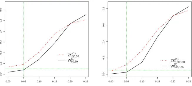
The percentage of rejections from 1,000 independent simulations when the size of the test is fixed at 0.05 are reported in Figures 3.1 and 3.2 as power curves that are functions ofδ1 andδ2 whenn =m = 50and 100.
These figures also display the number of rejections of the ZS test for the classical hypothesis (3.1) (which corresponds toH0(j)with∆j = 0). From this, the following conclusions can be drawn.
1. The tests ofH0(j)based onWˆ(1)m,nexhibited the behaviour predicted by (2.16), even for relatively small values ofnand m. Focusing on the tests of H0(j) with results displayed in Figure 3.1, we observed that the empirical rejection rate was less than nominal forkvX1 −v1Yk2 < ∆1 = 0.1, approximately nominal whenkv1X−v1Yk2= ∆1 = 0.1, and the power increased askvX1 −vY1k2began to exceed0.1.
In additional simulations not reported here, these results were improved further by taking larger values ofnandm.
2. Observe that with data generated according to Scenario 2,H0(2)is satisfied whileH0(3)is not satisfied for values ofδ2 >0.3155. This scenario is seen in Figure 3.2 where the tests forH0(2) exhibited less than nominal size, as predicated by (2.16), even in the presence of differences in higher-order eigenfunctions.
The tests ofH0(3)performed similarly to the tests ofH0(1).
3. The self-normalized ZS test for the classical hypothesis (3.1), which is based on the bootstrap, per- formed well in our simulations, and exhibited empirical size approximately equal to the nominal size whenkvX1 −vY1k2= 0, and increasing power askv1X−v1Yk2increased. For the sample sizem=n= 50 it overestimated the nominal level of5%. Interestingly, the proposed tests tended to exhibit higher power than the ZS test for large values ofkvX1 −vY1k2, even while only testing for relevant differences. Addi- tionally, the computational time required to perform the proposed test is substantially less than what is required to perform the ZS test, since it does not need to employ the bootstrap.
0.00 0.05 0.10 0.15 0.20 0.25
0.00.10.20.30.40.50.6
ZS50,50(1) W50,50(1)
0.00 0.05 0.10 0.15 0.20 0.25
0.00.20.40.60.8
ZS100,100(1) W100,100(1)
Figure 3.1: Percentage of rejections (out of 1,000 simulations) of the self-normalized statistic of Zhang and Shao (2015) for the classical hypotheses (3.1) (denotedZSn,m(1) ) and the new test (2.13) for the relevant hypo- hteses (2.3) (denoted byWm,n(1)) as a function ofδ1 in Scenario 1. In the left hand paneln=m = 50, and in the right hand paneln = m = 100. The horizontal green line is at the nominal level 0.05, and the vertical green line atδ1 = 0.05indicates the case whenkvX1 −v1Yk2 = ∆1 = 0.1.
.
0.0 0.5 1.0 1.5 2.0
0.00.10.20.30.4
ZS50,50(2) W50,50(2) ZS50,50(3) W50,50
(3)
0.0 0.5 1.0 1.5 2.0
0.00.10.20.30.40.50.6 ZS100,100(2) W100,100(2) ZS100,100(3) W100,100
(3)
Figure 3.2: Percentage of rejections (out of 1,000 simulations) of the self-normalized statistic of Zhang and Shao (2015) for the classical hypotheses (3.1) (denoted ZSn,m(j) , j = 2,3) and the new test (2.13) for the relevant hypohteses (2.3) (denoted byWm,n(j) ,j= 2,3) as a function ofδ2in Scenario 2. In the left hand panel n = m = 50, and in the right hand paneln = m = 100. The horizontal green line is at the nominal level 0.05, and the vertical green line atδ2= 0.3155indicates the case whenkvX3 −v3Yk2= ∆1 = 0.1.
3.1 Multiple comparisons
In order to investigate the multiple testing procedure of Section 2.3,XandY samples were generated accord- ing to model (3.2) withn = m = 100in two situations: one withδ1 = 0.0504915 andδ2 = 0.3155, and another withδ1= 0.25andδ2 = 2. In the former case,kvXj −vjYk2 ≈0.1forj = 1, . . . ,4, while in the latter casekvjX −vjYk2 >0.1,j = 1, . . . ,4. We then applied tests ofH0,pin (3.1) with∆j = 0.1forj= 1, . . . ,4 and variedp= 1, . . . ,4. These tests were carried out by combining the marginal tests for relevant differences of the respective eigenfunctions using the standard Bonferroni correction as well as the Holm–Bonferroni correction. Empirical size and power calculated from 1,000 simulations with nominal size0.05for each value ofpand correction are reported in Table 3.1. It can be seen that these corrections controlled the family-wise error rate well. The tests still retain similar power when comparing up to four eigenfunctions, although one may notice the declining power as the number of tests increases.
δ1 δ2 j= 1 2 3 4 0.0504915 0.3155 B 0.036 0.021 0.018 0.017
HB 0.037 0.036 0.024 0.025
0.25 2 B 0.750 0.678 0.668 0.564
HB 0.750 0.798 0.716 0.594
Table 3.1: Rejection rates from 1,000 simulations of testsH0,j with nominal level0.05forj = 1, . . . ,4and Bonferroni (B) and Holm–Bonferroni (HB) corrections.
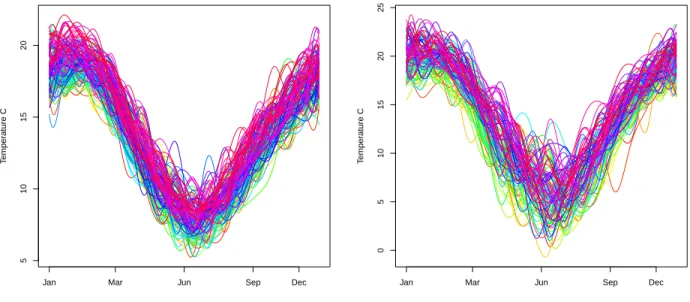
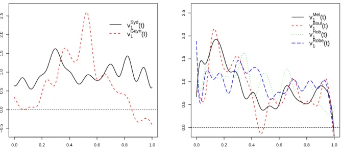
4 Application to Australian annual temperature profiles
To demonstrate the practical use of the tests proposed above, the results of an application to annual minimum temperature profiles are presented next. These functions were constructed from data collected at various measuring stations across Australia. The raw data consisted of approximately daily minimum temperature measurements recorded in degrees Celsius over approximately the last 150 years at six stations, and is available in theRpackagefChange, see S¨onmez et al. (2017), as well as fromwww.bom.gov.au. The exact station locations and time periods considered are summarized in Table 4.1. In addition, Figure 4.1 provides a map of eastern Australia showing the relative locations of these stations.
Location Years
Sydney, Observatory Hill 1860–2011 (151) Melbourne, Regional Office 1856–2011 (155)
Boulia, Airport∗ 1900–2009 (107)
Gayndah, Post Office 1905–2008 (103) Hobart, Ellerslie Road 1896–2011 (115)
Robe 1885–2011 (126)
Table 4.1: Locations and names of six measuring stations at which annual temperature data was recorded, and respective observation periods. In brackets are the numbers of available annual temperature profiles. The 1932 and 1970 curves were removed from the Boulia series due to missing values.