A Combined Nonparametric Test for Seasonal Unit Roots

IHS Economics Series Working Paper 303

March 2014

A Combined Nonparametric Test for Seasonal Unit Roots

Robert M. Kunst

Impressum Author(s):

Robert M. Kunst Title:

A Combined Nonparametric Test for Seasonal Unit Roots ISSN: Unspecified

2014 Institut für Höhere Studien - Institute for Advanced Studies (IHS) Josefstädter Straße 39, A-1080 Wien

E-Mail: o ce@ihs.ac.atffi Web: ww w .ihs.ac. a t

All IHS Working Papers are available online: http://irihs. ihs. ac.at/view/ihs_series/

This paper is available for download without charge at:

https://irihs.ihs.ac.at/id/eprint/2251/

A Combined Nonparametric Test for Seasonal Unit Roots

Robert M. Kunst

303

Reihe Ökonomie

Economics Series

303 Reihe Ökonomie Economics Series

A Combined Nonparametric Test for Seasonal Unit Roots

Robert M. Kunst March 2014

Institut für Höhere Studien (IHS), Wien

Contact:

Robert M. Kunst

Department of Economics and Finance Institute for Advanced Studies Stumpergasse 56

1060 Vienna, Austria

: +43/1/599 91-255 email: robert.kunst@ihs.ac.at and University of Vienna

Founded in 1963 by two prominent Austrians living in exile – the sociologist Paul F. Lazarsfeld and the economist Oskar Morgenstern – with the financial support from the Ford Foundation, the Austrian Federal Ministry of Education and the City of Vienna, the Institute for Advanced Studies (IHS) is the first institution for postgraduate education and research in economics and the social sciences in Austria. The Economics Series presents research done at the Department of Economics and Finance and aims to share “work in progress” in a timely way before formal publication. As usual, authors bear full responsibility for the content of their contributions.

Das Institut für Höhere Studien (IHS) wurde im Jahr 1963 von zwei prominenten Exilösterreichern – dem Soziologen Paul F. Lazarsfeld und dem Ökonomen Oskar Morgenstern – mit Hilfe der Ford- Stiftung, des Österreichischen Bundesministeriums für Unterricht und der Stadt Wien gegründet und ist somit die erste nachuniversitäre Lehr- und Forschungsstätte für die Sozial- und Wirtschafts- wissenschaften in Österreich. Die Reihe Ökonomie bietet Einblick in die Forschungsarbeit der Abteilung für Ökonomie und Finanzwirtschaft und verfolgt das Ziel, abteilungsinterne Diskussionsbeiträge einer breiteren fachinternen Öffentlichkeit zugänglich zu machen. Die inhaltliche

Abstract

Nonparametric unit-root tests are a useful addendum to the tool-box of time-series analysis.

They tend to trade off power for enhanced robustness features. We consider combinations of the RURS (seasonal range unit roots) test statistic and a variant of the level-crossings count.

This combination exploits two main characteristics of seasonal unit-root models, the range expansion typical of integrated processes and the low frequency of changes among main seasonal shapes. The combination succeeds in achieving power gains over the component tests. Simulations explore the finite-sample behavior relative to traditional parametric tests.

Keywords

Seasonality, nonparametric tests, visualization, time series

JEL Classification

C12, C14, C22

Contents

1 Introduction 1

2 Jittered seasonal phase plots

2.1 The quarterly case ... 3 2.2 The monthly case ... 8

3 Various models of seasonality and their phase plots 9

3.1 Deterministic seasonality ... 9 3.2 Periodic models ... 10 3.3 An experiment with a structural break ... 13

4 A nonparametric test for seasonal unit roots 14

5 Empirical applications 26

6 Summary and conclusion 30

References 31

1 Introduction

The current literature on seasonal time series (see Ghysels and Osborn, 2001, or Caporale et al. 2012, for example) ascribes the origin of the basic discrimination problem among conflicting paradigms for the generation of seasonal features to Hylleberg (1986).

The three main model worlds of concern are: (a) determin- istic seasonal variation, as customarily expressed via seasonal dummy variables; (b) seasonal unit roots and seasonal integra- tion; (c) stochastic stationary cyclical variation. A distinctive feature among these concepts is their implication with regard to forecasts of seasonal patterns. Deterministic seasonal patterns in an otherwise stationary environment entail that the sample aver- age of seasonal shapes is the best predictor for future shapes at longer horizons. Seasonal integration emphasizes the importance of the most recent pattern as a shape predictor, even though this prediction will face increasing uncertainty at increasing hori- zon and persistent shape changes are to be expected. Stationary cyclical variation permits some short-run extrapolation of pat- terns but it will imply trivial predictions at longer horizons.

The most important statistical tools for discriminating among

these main concepts of seasonal time-series generators were cre-

ated in the 1990s: the HEGY test by Hylleberg et al. (1990),

the test by Canova and Hansen (1995), and some further con-

tributions that are conveniently summarized by Ghysels and

Osborn (2001). These tests are parametric tests that build on

Gaussian likelihoods and optimize power properties for specific

designs. By contrast, nonparametric tests aim at increased ro- bustness at the price of reduced power.

Variance-ratio tests for seasonal unit roots were considered by Taylor (2005) who generalized the testing concept by Bre- itung (2002) to the seasonal case. Whereas these tests achieve additional robustness, they cannot be viewed as narrow-sense nonparametric. Kunst and Franses (2011) extended the non- parametric RUR (range unit-root) test by Aparicio et al. (2006) to the seasonal case. The test suggested here combines their RURS (RUR seasonal) test with another nonparametric unit-root testing idea that was investigated by Burridge and Guerre (1996). Their test relies on counting zero crossings and was mod- ified by Garc´ıa and Sans´ o (2006).

We provide an additional motivation for our selection of com- ponent tests in our new test by first presenting the idea of jit- tered seasonal phase plots. These plots are constructed as fol- lows. First, the information on seasonal shapes is condensed into classes, and then the transition patterns between these classes are recorded.

The paper is organized as follows. Section 2 introduces the jittered seasonal phase plots as a visualization tool. Section 3 reviews the typical patterns created by classes of seasonal gener- ators. Section 4 considers the nonparametric combination test.

Section 5 applies the methods to exemplary time series. Section

6 concludes.

2 Jittered seasonal phase plots

2.1 The quarterly case

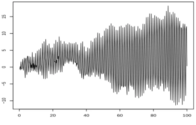
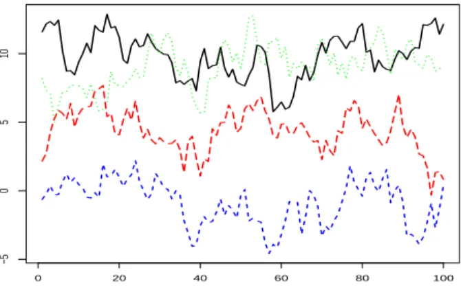
Figure 1 shows the typical visualization of a seasonal time series as a time plot: the partial realization, an element of the space

with sample size n, is drawn as a curve in

. The generating model is a quarterly Gaussian seasonal random walk x

= x

+ε

for t

0 with x

= 0,

t

0 as starting conditions. The experienced user is likely to decide for a seasonal unit-root model on the basis of Figure 1.

0 20 40 60 80 100

−10−5051015

Figure 1: Time plot of a realization of a seasonal random walk.

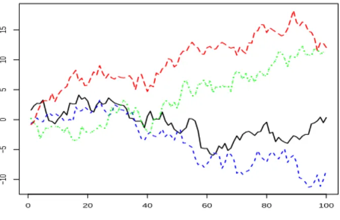
A characteristic feature of seasonal unit-root processes are the

infrequent but persistent changes in the rank position of quarters

(in the case of quarterly data). These are emphasized visually

if the series is represented by four quarterly series: the spring

series, the summer series etc. For the example of Figure 1, Figure

2 provides this representation.

0 20 40 60 80 100

−10−5051015

Figure 2: Time plot by seasons of a realization of a seasonal random walk.

The idea of counting the intersections of quarterly plots in or- der to obtain a non-parametric statistic for discriminating among the main seasonal generating models was pursued by Kunst (2009). Each of these crossings represents a change of the qual- itative seasonal pattern, in the sense that, for example, stronger sales of a product during the spring season give way to higher sales in summer. For the following, we convene that changes in the seasonal pattern are reflected in a reversal of ranking between two successive quarters.

Figure 3 reproduces the eight possible qualitative seasonal pat-

terns that we use here. The cases have been coded conveniently as

triples of binary numbers, using ‘1’ for an increase between quar-

ters and ‘0’ for a decrease. Several alternative discretizations are

conceivable. Even in the 101 pattern, for example, it may make

sense to separate cases with a spring peak from those with a fall

peak, and with a summer trough from a winter trough. This,

however, would increase the number of classes to 24. Note that the direction from the last quarter of a year to the first quarter of the following year has also been excluded from the classification.

This follows the idea that seasonality should be viewed indepen- dently from the year-to-year trend. Thus, the 111 pattern should not be subdivided into cases with a strong slump at the beginning of the year and cases with a persistent upward movement. Again, the increase in the number of classes to 16 would be inconvenient.

000 001 010

011 100 101

110 111

Figure 3: The eight qualitative seasonal patterns for quarterly data.

Discretization of the sample space into 8 classes, of course, en- tails a considerable loss in information and can only be justified if the result assists in the discrimination problem of concern. It is fairly simple to simulate some basic time-series models and to generate connected phase plots from the trajectories. Unfortu- nately, even when large samples are generated, the usefulness of such graphs is limited. Basic properties that would be important for a reliable classification are not easily recognized. As a visual tool, these graphs do not convince.

A main problem in the simple phase plot is that it does not show the population within the classes. One suggestion would be to simply randomize the observations in an interval such as [m

0.4, m + 0.4], which would correspond to the technique of jittering that is widespread. A more sophisticated visualization is to distribute the observations that belong to class m according to their ‘depth’ within the class. Given that an observation is classi- fied to m according to increases or decreases in specific quarters, it can be said to be ‘deep’ in the class when these increases or decreases are large, while almost constant patterns can be seen as ‘shallow’. There are three quarter-to-quarter movements, and an observation may be deep regarding quarter 1-2 and shallow in other quarters. Several solutions may be considered.

We decided for a distribution according to maximum relative

depth, calculated from maximum absolute inter-quarter increases

or decreases. We experimented with shallow points in the center

of the interval and deep points at the boundaries as well as with

the reverse convention, and finally decided for the former, as it

tends to convey a slightly clearer picture. Thus, points in the center are the shallowest class members, and after an extended period in the class they tend to attain the boundaries.

There is no coercive convention for the left and right parts of the interval, [m

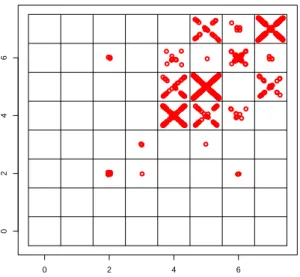
0.4, m) and (m, m + 0.4]. These could be used for observations that are deep regarding the first movement on the left and those deep in the second movement on the right, but this still would leave the third one undecided. We decided for uniform randomization, i.e. jittering in the literal sense. For sea- sonal unit-root processes, deep observations tend to be followed by deep ones, and this randomization tends to generate a St. An- drew’s cross or saltire, a pattern that sends a clear message to the observer. The result of this procedure is shown in Figure 4.

0 2 4 6

0246

Figure 4: Jittered phase diagram for pattern classes. Generating model is a

quarterly Gaussian seasonal random walk with 40,000 observations.

2.2 The monthly case

In principle, the monthly case can be handled in analogy to the quarterly case. The main difficulty in visualizing the phase plots is the large number of shape classes that is 2

if S denotes the seasonal periodicity. For quarters, 2

= 8 is a conveniently small number, while for months 2

= 2048 is quite impressive. Because of the limited resolution of the graphs, the cross shape within the bins is no longer recognizable and visual evaluation must rely on the patterns of transition among shapes exclusively.

Accordingly, we experimented with jittered plots for the monthly seasonal random walk. It appears that observations tend to clus- ter in specific areas close to the diagonal and that transitions across shapes are recognizeably rare. Such plots can be con- fronted with control plots that are generated from Gaussian white noise. Then, shape transitions become frequent, and all classes are represented, although not uniformly. In another control ex- periment, realizations of Gaussian random walks without any seasonal features tend to generate homogeneously filled squares.

Eyeballing is sure to discriminate such non-seasonal benchmarks

from the seasonal random walk.

3 Various models of seasonality and their phase plots

3.1 Deterministic seasonality

Whereas unit-root seasonality generates the hitherto highlighted features, i.e. rare transitions between bins and persistence within some bins, many seasonal cycles observed in the real world appar- ently support deterministic models with different characteristic features.

For example, temperature is unlikely to ever transit from a pattern with a summer peak and a winter trough to a reversal of extrema, at least in many moderate climates. Data are then likely to be classified into the ‘110’ pattern exclusively. Similarly, tourism data for a mountainous region may display twin-peak patterns with a preference for summer and winter tourism, al- though with low activity in early spring or in fall. This may correspond to the pattern coded as ‘101’.

A simple generating model for such deterministic seasonal variation is a stable ARMA model superseded with a repetitive cycle expressed via seasonal dummy variables. For exposition, we consider the generating model

x

= 0.4x

+

4

X

j=1

d

δ

+ ε

,

with standard Gaussian errors and δ

denoting the customary

seasonal dummy constants. For the deterministic pattern, we

impose the sequence (d

, . . . , d

) = (0, 8, 3, 10). Figure 5 provides

a time-series plot.

0 20 40 60 80 100

−50510

Figure 5: Time series plot for 400 observations generated from a deterministic seasonal process.

The corresponding plot by quarters is given in Figure 6. While the two peaking quarters 2 and 4 show some tendency to change their rankings, the low-activity quarter 1 remains at the bottom during the entire sampling interval.

The impression is confirmed in a jittered phase plot shown in Figure 7. There is a strong preference for one class, and occasional visits to other classes remain episodic.

3.2 Periodic models

If the generating law of the process varies with the season, the

process is called periodic. For details, see Ghysels and Osborn

(2001, Ch. 6) or Franses (1996). The simplest model of this type

0 20 40 60 80 100

−50510

Figure 6: Time plot by seasons of a realization of a process with deterministic seasonality.

0 2 4 6

0246

Figure 7: Jittered phase diagram for pattern classes. Generating model is a

process with deterministic seasonal variation and 40,000 observations.

is the periodic AR(1) model:

x

= φ

x

+ ε

,

with s = t mod S + 1. Whereas the model is not so often used on economic time series, a specific type of periodic process, the periodically integrated process, is of interest as it bridges the gap between seasonal integration and purely deterministic seasonality.

The periodic AR(1) process can be shown to be periodically integrated iff

S

Y

s=1

φ

= 1,

in which case x

displays some typical features of a seasonally integrated process, whereas the separate seasons are now cointe- grated, which they are not in the seasonal random walk model.

Because of this property, periodically integrated variables are usu- ally difficult to distinguish from seasonally integrated variables by typical statistical tests for seasonal integration, such as the HEGY test due to Hylleberg et al. (1990).

In an exemplary experiment, we generated 40,000 observa- tions from a periodically integrated process with S = 4 and (φ

, . . . , φ

) = (1, 0.25, 1, 4). The concomitant jitter plot is not shown here because of its high bit size at an acceptable resolu- tion. This jitter plot reflects the construction principle. If the variable has a positive value at the end of a year, it tends to fall from the first to the second quarter and to rise from the third to the fourth quarter, with the movement in between undetermined.

Thus, the jittered phase plot shows a clear emphasis on the bins

# 4 and # 6, with frequent transitions between these two. The

bins # 1 and # 3 constitute a similar pattern for negative values.

Thus, the bin pair #1 and #3, and the bin pair #4 and #6 form two loosely related subsystems. Within all bins, the jittered plot displays blotches rather than saltires and thus does not support seasonal unit roots visually. The graphical procedure clearly dis- criminates the periodic model from the seasonally integrated one.

Comparable patterns are also found with different designs for the coefficient sequence.

3.3 An experiment with a structural break

Balcombe (1999) pointed at the low power of seasonal unit- root tests in the presence of structural breaks. Just as in the case of unit-root tests for the traditional root at one, it should be noted that data-generating processes with breaks are neither in the null nor in the alternative of the original unit-root tests, thus it is uncertain whether the outlined property can really be regarded as a problem of low power. Rather, the issue appears to be a robustness problem. If the original classes of processes are perturbed, the tests that are designed for these classes fail to classify correctly.

In detail, Balcombe perturbs a random walk with added deterministic variation by a change in the seasonal pattern in the middle of the sample, with the strength of perturbation indicated by a parameter α:

∆x

=

4

X

j=1

(1

αD

)d

δ

+ ε

,

with (d

, . . . , d

) = (0, 1, 1,

D

= 0 for t < T /2 and

D

= 1 for t

T /2. The perturbation parameter is varied over the set

1, 2}. α = 0 represents the undisturbed case, for α = 1 seasonality disappears after the break, while for α = 2 the seasonal pattern is reversed after the break.

Because of the excessive size of the plot files, the seasonal jitter plots for this generating process cannot be shown here. By con- struction, the method is unaffected by any time reversal, and thus it cannot distinguish whether variation diminishes or increases.

The case α = 0 is clearly reflected by deterministic spots at the dominant bins # 4 and # 6, which often alternate as the second and third quarter have identical means. The case α = 2 reflects the bins # 4 and # 6 that dominate for small t as well as the bins # 1 and # 3 that dominate at large t. The intermediate case α = 1 shows non-seasonal blotches, as the non-seasonal second half dilutes the patterns in the first half. In none of the three cases, graphs would seriously indicate seasonal unit roots. Thus, in a sense, the visualization is unaffected by the discrimination problem of the parametric test.

4 A nonparametric test for seasonal unit roots

We first note that the classification decision based on the jittered plots mainly depends on two features: (i) the transition frequency across shape classes and (ii) the precision of the saltire shapes.

Whereas the following presentation is restricted to the quarterly

case, it is straight forward to generalize toward other frequencies.

In particular, we note that the fact that the visualization in the phase plot cannot show the within-bin patterns does not preclude the numerical value of the corresponding test statistic from being calculated.

Concerning the transition frequency, it is convenient to start from the case that the data-generating process is a seasonal ran- dom walk. The event of a shape transition, for example

x

> x

, x

< x

,

with x

denoting the quarter i in year j, clearly is equivalent to x

x

> 0, x

x

< 0.

In a seasonal random walk, the quarters represent independent random walks. The difference between quarters is then a random walk itself, so the above event is a zero crossing for the random walk x

x

.

Some facts on the distribution of zero crossings in random walks are known from the literature (Burridge and Guerre, 1996, Garc´ıa and Sans´ o , 2006). In particular, Burridge and Guerre (1996) showed that the modified crossings count K

(0) = σ ˆ

\

MAD T

T

X

t=1

I(X

x, X

> x)+I(X

> x, X

x)

is asymptotically distributed as

(0, 1)|. Here, ˆ σ denotes an

estimate of the standard error of the increments ∆X

, whereas

MAD is an estimate of their absolute first moments. These two

correction factors are suggested to be formed empirically as

ˆ

σ =

v u u t

T

T

X

t=1

(∆X

)

, (1)

MAD =

T

T

X

t=1

|∆Xt|.

(2)

Garc´ıa and Sans´ o (2006, GS) then generalized this result to trend-corrected random walks, for which the modified crossings statistic converges to a Rayleigh distribution. In particular, how- ever, GS showed that replacing the sample variance in formula (1) by a long-range variance in the vein of variance-ratio tests or the popular unit-root test by Phillips and Perron (1988) succeeds in making the test robust to autocorrelation in the in- crements under the null of a unit root. The main argument in their proof relies on a result by Akonom (1993). In other words, the test that was strictly valid only for random walks in the ver- sion of Burridge and Guerre (1996) now becomes a test for the null of a first-order integrated process, in symbols I(1). In the following, we refer to the modified statistic as ˜ ζ

and to the original statistic as ζ

.

The modified statistic K

(0) constitutes our first nonpara- metric test statistic ζ

or ζ

. Its asymptotic distribution under the null of a seasonal random walk is known, though we will not exploit this property explicitly.

Concerning the precision of the saltire, we form a second non-

parametric test statistic ζ

from the median distance between

observations in the (i, j ) bin and the saltire form. Clearly, this

distance can be envisaged as the distance of the absolute point

(|˜ x

x

x denotes a properly nor- malized observation relative to the center of the corresponding bin. This distance, in turn, equals 2

∆|˜ x

in the diagonal (i, i) bins, and its average should converge to an absolute moment of a distribution of increments.

We note, however, that the bins have been scaled to minima and maxima. Such maxima are known to expand at the rate of T

for random walks and at a much slower rate of log T for stationary Gaussian variables. Thus, the average of the incre- ments in a scaled world approaches zero at a rate of T

for random walks, while its properties depend on characteristics of the data-generation process including error distributions for sta- tionary variables. Accordingly, the nonparametric test statistic ζ

is defined as T

multiplied by the medium distance of ob- servations and the saltire. We opt for the median rather than the mean for the sake of distributional robustness. A compara- ble nonparametric test statistic based on a similar principle was suggested by Aparicio et al. (2006, AES).

It is unfortunate that a robustification step comparable to the

correction by GS for the original suggestion by Burridge and

Guerre (1996) is not available for the AES test. This property

is rooted deeply in the construction principle of the tests. The

level-crossings count is sensitive to moments of the generating

distribution, which are then adjusted for by a correction factor,

and this factor is in turn robustified in the GS version. In the

AES test, by contrast, the adjustment term cancels out, and the

distribution of the test statistic is independent of the moment

properties of the generating law for pure random walks.

It pays to reconsider the shapes that we encountered by sim- ulation in Section 2 in the light of this discussion. For a seasonal random walk, the saltire shape is approximated as the sample size increases, with the average distance from the saltire decreas- ing. For a non-seasonal random walk, both the horizontal and vertical directions of the bins expand at the rate T

, and the bins are densely filled. For white noise, both directions expand slowly, and the bins are filled in a circular fashion, with points in the corners remaining rare.

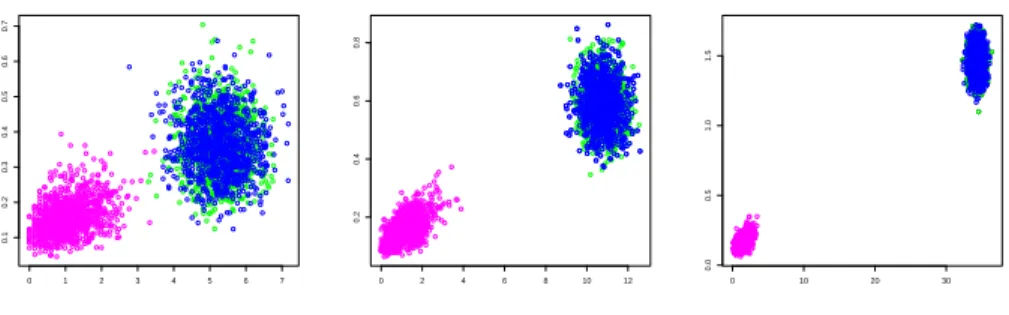
A crude demonstration of the power of this test is provided in Figure 8. 1000 replications of Gaussian random walks, Gaussian seasonal random walks, and Gaussian white noise were gener- ated, and all realizations of both test components were plotted.

It appears that even at the smallest sample size of 25 years does the test show some power. For the larger samples, discrimination between the pattern persistence of the seasonal unit-root process and the other generating laws become almost perfect. Instruc- tive visualizations of this type are routinely used in discriminant analysis (see, for example, James et al., 2013), where a linear decision boundary is determined. Similarly, we shall introduce a combination test that corresponds to such a boundary line.

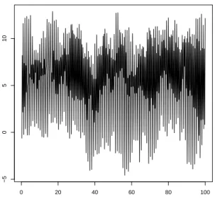
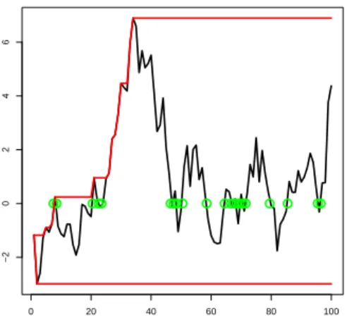
A convenient visualization of the workings of the two test

statistics is provided in Figure 9. The occasions where the cross-

ings count increases are marked as well as the points where new

maxima or minima occur. The plot may insinuate that random-

walk realizations with many crossings and thus a large value of ζ

0 1 2 3 4 5 6 7

0.10.20.30.40.50.60.7

0 2 4 6 8 10 12

0.20.40.60.8

0 10 20 30

0.00.51.01.5

Figure 8: Scatter plots of realizations of the two test statistics ζ

and ζ

derived from the jittered phase plots. Generating laws are the seasonal ran- dom walk (magenta), the random walk (green), and white noise (blue). Left graph T = 100, central graph T = 400, right graph T = 4000.

have a smaller expansion rate and thus lower ζ

. For very small samples, the two test statistics are thus negatively correlated by construction. It appears, however, that this strong negative de- pendence soon disappears as the sample size increases.

The statistics ζ

and ζ

process different information. Whereas good or even optimal combinations of individual tests can be constructed by the Bonferroni principle, we here insist on the convenient simplicity of a combination that is evaluated quickly.

A linear combination such as ζ

+ cζ

may have higher power than

individual tests. Whereas relative scales would suggest c = 7,

the comparative power simulations favored a larger value around

c = 17. From the various power simulations at varying sample

sizes, we show two exemplary plots in Figure 10. Test power is

seen to increase rapidly as c approaches values around c = 17

from below and to decrease slowly as c increases further. The

power maxima appear as a nearly straight line and recommend

0 20 40 60 80 100

−20246

Figure 9: Exemplary realization of a random walk, with new extrema (for ζ

) marked as well as zero passages (for ζ

).

a constant value of c. It is of some interest, however, that lower values of c sometimes occur very close to the null. Low optimal c is also typical at a large distance from the null, where the ζ

test is often unable to achieve power close to one.

In the following, the statistic

ζ = ζ

+ 17 ζ

18

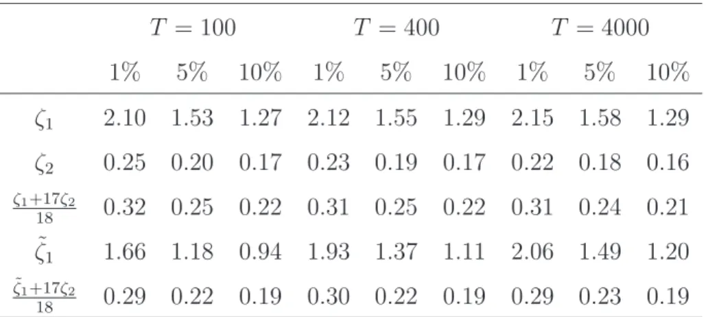
will be in focus. For the highly non-standard null distribution of these statistics, Table 1 provides some quantiles.

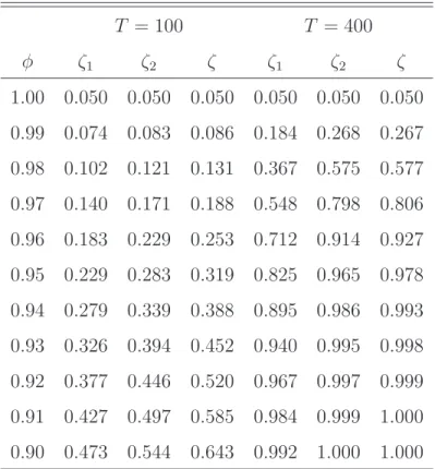
Based on the simulated quantiles, Table 2 adds some sim- ple power simulations. Test power is investigated along the ray through the alternative

x

= φx

+ ε

,

with φ varying over 0.9 + j

0.01 with j = 0, . . . , 10, such that

j = 10 represents the null and j = 0 implies φ = 0.9. This rather

0.00 0.02

0.04 0.06

0.08

0.10 0 5

10 15

20 0.75

0.80 0.85 0.90 0.95 1.00

0.00 0.02

0.04 0.06

0.08 0.10

5 10

15 20 0.7

0.8 0.9 1.0

Figure 10: Ratios of test power along generated models x

= φx

+ ε

, for φ = 1

φ ˜ and ˜ φ on the y–axis. Tests are based on linear combinations ζ

+cζ

, with c on the x–axis. For given ˜ φ, power is divided by the maximum, such that a value of 1 on the z–axis indicates maximum power. Left graph for T = 100, right graph for T = 400.

Table 1: Significance points for the nonparametric tests.

T = 100 T = 400 T = 4000

1% 5% 10% 1% 5% 10% 1% 5% 10%

ζ

2.10 1.53 1.27 2.12 1.55 1.29 2.15 1.58 1.29 ζ

0.25 0.20 0.17 0.23 0.19 0.17 0.22 0.18 0.16

ζ₁+17ζ₂

18

0.32 0.25 0.22 0.31 0.25 0.22 0.31 0.24 0.21 ζ ˜

1.66 1.18 0.94 1.93 1.37 1.11 2.06 1.49 1.20

ζ˜₁+17ζ₂

18

0.29 0.22 0.19 0.30 0.22 0.19 0.29 0.23 0.19

crude simulation design corresponds to the very basic seasonal unit-root test that was suggested originally by Dickey et al.

(1984), which is rarely used nowadays. Nonetheless, power turns out to be surprisingly good, although lower than for the para- metric HEGY test or the test by Dickey et al. (1984), which was constructed particularly along the same ray and has the best power here. The combined version ζ =

dominates the single tests convincingly, sometimes excepting an area close to the null, where ζ

alone shows a slight advantage. On the other hand, ζ

shows unsatisfactory performance in small samples at comparatively large distance from the null. Also Kunst (2009) and Kunst and Franses (2011) report low power in many di- rections for a non-parametric test that relies on a principle similar to ζ

.

We note that Table 2 indeed evaluates the power for the un- corrected original statistics ζ

and ζ and not for the adjusted statistics ˜ ζ

and ˜ ζ. Not much is lost, however, in this simple design if the adjustment is applied here. The situation changes when autocorrelation is present under the null.

A known problem with both original nonparametric unit-root

tests ζ

and ζ

and thus also with the combined ζ is that the

statistical properties are sensitive to deviations from the pure

seasonal random walk model under the null. In other words, the

test becomes non-similar. The experiments reported in Table

3 confirm this problem. If the SRW generating mechanism is

replaced by x

= x

+ u

with u

stable autoregressive, the

test becomes undersized for negative and positive autocorrelation,

Table 2: Power properties of the nonparametric tests.

T = 100 T = 400

φ ζ

ζ

ζ ζ

ζ

ζ

1.00 0.050 0.050 0.050 0.050 0.050 0.050 0.99 0.074 0.083 0.086 0.184 0.268 0.267 0.98 0.102 0.121 0.131 0.367 0.575 0.577 0.97 0.140 0.171 0.188 0.548 0.798 0.806 0.96 0.183 0.229 0.253 0.712 0.914 0.927 0.95 0.229 0.283 0.319 0.825 0.965 0.978 0.94 0.279 0.339 0.388 0.895 0.986 0.993 0.93 0.326 0.394 0.452 0.940 0.995 0.998 0.92 0.377 0.446 0.520 0.967 0.997 0.999 0.91 0.427 0.497 0.585 0.984 0.999 1.000 0.90 0.473 0.544 0.643 0.992 1.000 1.000

Generating model is x

= φx

+ ε

. Significance level is 5%. φ = 1 is the

null.

Table 3: Power properties for the nonparametric tests for autocorrelated increments in the versions without long-run variance adjustment.

θ =

θ = 0 θ = 0.5

φ ζ

ζ

ζ ζ

ζ

ζ ζ

ζ

ζ

1.0 0.041 0.042 0.043 0.050 0.050 0.050 0.044 0.035 0.036 0.98 0.084 0.099 0.101 0.102 0.121 0.131 0.083 0.096 0.094 0.96 0.137 0.185 0.190 0.183 0.229 0.253 0.143 0.195 0.193 0.94 0.204 0.288 0.296 0.279 0.339 0.388 0.227 0.314 0.324 0.92 0.283 0.390 0.406 0.377 0.446 0.520 0.325 0.444 0.467 0.9 0.364 0.485 0.510 0.473 0.544 0.643 0.431 0.555 0.600 Generating model is x

= φx

+ u

, u

= θu

+ ε

. Significance level is 5%.

φ = 1 is the null. Sample size T = 100.

with the size bias persisting at slightly larger samples. The size bias is reflected in somewhat lower power under the alternative.

By contrast, if the long-run variance correction is implemented, the distortion problems mostly disappear. We note that the com- ponent test based on ζ

cannot be adjusted and that thus the com- bined test inherits problems from its typically strongly weighted component. The adjusted portion ˜ ζ

, however, succeeds in re- moving a good part of the distortion. Another feature, however, makes Figure 11 even more interesting. In these simulations, we ran control simulations based on the traditional parametric HEGY test. Actually, we considered two versions of the HEGY test: first, an F test for the seasonal unit roots at

second, an F test for the same seasonal unit roots, although under

0.90 0.92 0.94 0.96 0.98 1.00

0.00.10.20.30.40.50.60.7

0.95 0.96 0.97 0.98 0.99 1.00

0.00.20.40.60.81.0

Figure 11: Power function for T = 100 and T = 400. Black: ˜ ζ

; red:

ζ

; green: ζ

. Light blue dashes: a HEGY variant. Generating model is x

= φx

+ u

, u

= θu

+ ε

, θ = 0.25j, j =

3.

the incorrect assumption of a unit root at +1. The power perfor- mance of both HEGY versions is very similar. The HEGY test is clearly beaten by the nonparametric tests under investigation.

We note that the power performance of the HEGY test agrees

quite well with literature sources, thus the difference between the

tests is not due to specific problems of the parametric tests but

rather to the effect of additional power of range expansion tests

that was also emphasized by AES. We note that the dominance

of the test ˜ ζ shrinks as T increases, and the HEGY test actually

dominates at larger distance from the null. The effect appears

to be at odds with the usual statistical test construction that

is based on asymptotic optimization, and it is difficult to inter-

pret. A tentative reason may be that the nonparametric tests

concentrate on the true classification features of interest, such as

zero crossings and range expansion, while the parametric tests

are limited by the precision of the regression estimates.

5 Empirical applications

Whereas the simulated charts are mostly based on relatively large samples, empirical data sets typically are much shorter, whether they are taken from economics or from other disciplines.

Austrian industrial production is a quarterly variable that is available from 1957. The left panel of Figure 12 shows the seasonal jitter plot for the years 1957–2011. The seasonal pat- tern shows some variation, but it usually returns to its basic shape quickly. A blurred saltire forms in bin # 5, which rep- resents the activity troughs during summer vacation and in the cold start of the year, with rising activity during the second and fourth quarters. The values of the test statistics are (˜ ζ

, ζ

, ζ) = ˜ (0.27, 0.17, 0.17). These values are in the non-rejection region, maybe excepting ζ

which provides weak evidence for rejection, as it is close to the 10% quantile.

The Austrian unemployment rate according to national definition—

the international or OECD definition yields a different rate that is available for a much shorter time span only—is a variable that has been compiled monthly since January 1950. Because of em- ployees in tourism, agriculture, and construction, this variable has quite strong seasonality. The right panel of Figure 12 shows the jitter chart of quarterly averages over the original months.

The rather clear saltire may be in accordance with seasonal unit

roots, although all observations are in the same shape class. The

values of the test statistics are here (˜ ζ

, ζ

, ζ) = (0, ˜ 0.16, 0.15), again indicating the non-rejection region.

0 2 4 6

0246

0 2 4 6

0246

Figure 12: Jittered phase plot for Austrian industrial production 1957–2011 and for the Austrian unemployment rate 1950–2011, quarterly observations.

The left panel of Figure 13 provides an example for a variable with weak seasonality. Rainfall (precipitation) measurements at the location of Heathrow in the United Kingdom are expected to reflect some degree of seasonality, as rainfall maxima and minima are often concentrated in specific months or quarters. For the graph, the original monthly series was aggregated into quarters, but the monthly version can also be inspected and gives a similar impression. The values of the test statistics are now (˜ ζ

, ζ

, ζ) = ˜ (2.60, 0.49, 0.60), and the test safely rejects seasonal unit roots.

By contrast, the right panel of Figure 13 shows the jitter plot for the air temperature at the same location. This variable pro- vides an example for purely deterministic seasonality with almost negligible dependence among seasonal pattern in adjacent years.

Four symmetric spots in the bin # 6 represent the repetitive cy-

cle of rise-rise-fall that is observed annually with no exception.

Even for monthly data, the regularity remains striking, though changes in rank are slightly more common. Here, the values of the test statistics are (˜ ζ

, ζ

, ζ) = (0, ˜ 0.21, 0.20), with ζ

playing a key role in rejecting seasonal unit roots.

0 2 4 6

0246

0 2 4 6

0246

Figure 13: Jittered phase plots for precipitation and for temperature at Heathrow, 1948–2011.

Core macroeconomic time series, such as gross domestic prod-

uct (GDP) are sometimes even shorter than unemployment and

industrial production, because of slight changes in definition, even

when longer series are available in principle. The two GDP series

analyzed in Figure 14 were naively concatenated from shorter ho-

mogeneous segments. The values of the test statistics (˜ ζ

, ζ

, ζ) ˜

are (0.35, 0.16, 0.17) for the Austrian case and (0.25, 0.19, 0.19)

for the British data. The Austrian sample, although short, is

well in line with the idea of seasonal unit roots, as the strong

temperature cycle with harsh winters affects the dynamics of the

economy. Correspondingly, the test fails to reject. By contrast,

ζ

rejects for the U.K., where a milder climate enables spreading

0 2 4 6

0246

0 2 4 6

0246

Figure 14: Jittered phase plots for Austrian (left, 1964:1–1987:4, T = 96) and U.K. (right, 1957:1–2011:4, T = 220) GDP

.

It is of some interest to compare these test results to the outcome of tra- ditional parametric tests for seasonal unit roots. For example, the most straightforward test of that type is the HEGY test due to Hylleberg et al.

(1990), which rejects the unit root null for all variables considered in this sec-

tion, excepting the GDP series that are rather short. It should be conceded,

however, that HEGY results vary somewhat across lag-order specifications

for augmenting terms.

6 Summary and conclusion

We demonstrate that the suggested nonparametric combination test tends to dominate its constituent component tests, and the suggested weight appears to be well chosen. It is surprising that in some designs the test even clearly dominates parametric tests for seasonal unit roots. Our results are in line with those of AES, whose simulations are quite supportive for their idea in traditional unit-root situations, as their RUR test often outperforms stan- dard tests, such as the Dickey-Fuller test. Our results are less in line with the simulations of Burridge and Guerre (1996) who delineate a gloomy picture for the power of their nonparametric tests, even if combined with traditional tests.

We are also able to demonstrate that the visualization by jit- tered phase plots is an appealing and potentially helpful tool in the investigation of the nature of seasonality in subannual time series. This tool unfolds its discriminatory power best when it is used together with traditional hypothesis tests. The slanted cross or saltire appears to be a well recognizable shape, and deviations from the pure form are easily spotted by the human eye.

A main problem with seasonality remains: good discrimina-

tion requires samples that are slightly larger than those that are

typically available. Really long time series are needed in order to

discriminate safely the case of pattern reversion from the case of

episodic pattern change. Applications to various data sets, how-

ever, insinuate that good seasonal unit-root processes are rare in

practice.

References

[1] Akonom, J. (1993): Comportement asymptotique du temps d’occupation du processus des sommes partielles. Annales de l’Institut Henri Poincar´e (B) Probabilit´es et Statistiques

57–81.

[2] Aparicio, F., Escribano, A., and A.E. Sipols (2006):

Range unit-root (RUR) tests: robust against nonlinearities, error distributions, structural breaks and outliers. Journal of Time Series Analysis

[3] Balcombe, K. (1999): Seasonal unit root tests with struc- tural breaks in deterministic seasonality. Oxford Bulletin of Economics and Statistics

[4] Breitung, J. (2002): Nonparametric tests for unit roots and cointegration. Journal of Econometrics

[5] Burridge, P., and E. Guerre (1996): The Limit Distri- bution of Level Crossings of a Random Walk, and a Simple Unit Root Test. Econometric Theory

[6] Canova, F., and B.E. Hansen (1995): Are seasonal pat- terns constant over time? A test for seasonal stability. Jour- nal of Business & Economic Statistics

[7] Caporale, M.C., Cunado, J., and L.A. Gil-Alana

(2012): Deterministic versus stochastic seasonal fractional

integration and structural breaks. Statistics and Computing

[8] Dickey , D.A., Hasza , D.P., and W.A. Fuller (1984):

Testing for Unit Roots in Seasonal Time Series. Journal of the American Statistical Association

[9] Franses , P.H. (1996): Periodicity and Stochastic Trends in Economic Time Series. Oxford University Press.

[10] Garc´ıa, A., and A. Sans´ o (2006): A generalization of the Burridge-Guerre Nonparametric Unit Root Test. Economet- ric Theory

[11] Ghysels, E., and D. Osborn (2001): The Economet- ric Analysis of Seasonal Time Series. Cambridge University Press.

[12] Hylleberg, S. (1986): Seasonality in Regression. Academic Press.

[13] Hylleberg , S., Engle , R.F., Granger , C.W.J., and B.S.

Yoo (1990): Seasonal integration and cointegration. Journal of Econometrics

, 215–238.

[14] James , G., Witten , D., Hastie , T., and R. Tibshirani (2013): An Introduction to Statistical Learning. Springer- Verlag.

[15] Kunst, R.M. (2009): A Nonparametric Test for Seasonal Unit Roots. Economics Series No. 233, Institute for Ad- vanced Studies, Vienna

[16] Kunst, R.M. , and P.H. Franses (2011): Testing for sea-

sonal unit roots in monthly panels of time series. Oxford

Bulletin of Economics and Statistics

, 469–488.

[17] Phillips , P.C.B., and P. Perron (1988): Testing for a unit root in time series regressions. Biometrika

[18] Taylor, A.M.R. (2005): Variance ratio tests of the seasonal

unit root hypothesis, Journal of Econometrics

Author: Robert M. Kunst

Title: A Combined Nonparametric Test for Seasonal Unit Roots Reihe Ökonomie / Economics Series 303

Editor: Robert M. Kunst (Econometrics)

Associate Editors: Michael Reiter (Macroeconomics), Selver Derya Uysal (Microeconomics)

ISSN: 1605-7996

Published 2014 by the Department of Economics and Finance, Institute for Advanced Studies (IHS), Stumpergasse 56, A-1060 Vienna •  +43 1 59991-0 • Fax +43 1 59991-555 • http://www.ihs.ac.at