Submitted in partial fulfillment of the requirements for the award of the degree of Master of Science in Medical Physics

Influence on different Monte-Carlo variances at the dose calculation and the impact to the commissioning

By

Jailan Alshaikhi

Thesis

Submitted in partial fulfillment of the requirements for the award of the degree of Master of Science in Medical Physics

August, 2010

Medical Faculty Mannheim

Ruprecht Karls University, Heidelberg

Adviser: Prof. Dr. Juergen Hesser

i

Declaration

I hereby affirm that I have written this thesis independently and without the use of resources other than those quoted. Cited and copied works are marked as such.

___________________________ ______________________

Jailan Alshaikhi Date

ii

Dedication

To my parents

iii

List of tables

Table 1 shows the gamma evaluation result for the square fields studied. ... 23 Table 2 shows the gamma result for rectangular fields ... 25 Table 3 shows the field shape, exposure parameters, gamma criteria and results for

irregular fields ... 27

Table 4 Calculation times for square fields at different variances ... 28

iv

List of figures

Figure 1: Screenshot of a dose comparison program. ... 9

Figure 2: An Elekta Synergy linear accelerator ... 13

Figure 3: The solid water phantom used for film exposure ... 14

Figure 4: Calculated dose distribution ... 17

Figure 5: Profile of calculated and measured dose distribution ... 19

Figure 6: Gamma evaluation result ... 21

Figure 7: Plot showing Monte Carlo calculation time as a function of variance and field size ... 29

Figure 8 shows the effect of using different variance in computing the dose on the dose volume histogram (DVH) of a patient (case 1) ... 30

Figure 9: shows the effect of using different variance in computing the dose on the DVH of

a patient (case 2)... 31

v

Table of Contents

Declaration ... i

Dedication ... ii

List of tables ... iii

List of figures ... iv

Acknowledgment ... vi

1. Introduction ... 1

1.1 Dose calculation methods ... 3

1.1.1 Indirect/ correction based dose computation method ... 4

1.1.2 Direct / model based dose computation methods ... 5

1.2 Monte Carlo dose calculation ... 6

1.3 Beam measurement and verification ... 8

2. Materials and methods ... 12

2.1 Dose calculation and delivery ... 12

2.2 Film calibration, comparison of calculated and measured dose ... 14

3. Result ... 16

3.1 Gamma analysis and computation time ... 16

3.2 Dosimetric effect of variance on DVH – IMRT clinical cases ... 30

4. Discussion ... 32

5. Conclusion... 36

References ... 37

vi

Acknowledgment

I wish to thank Prof. Dr. Juergen Hesser

Mr. Volker.Steil Mr. Kegel, Stefan Mrs. Klabes, Anika

Everybody in the Radiation Oncology Department

1

1. Introduction

The goal of radiation therapy is to kill tumor cells while reducing the injury to the normal tissues. The physician prescribe the target dose based on the experience gained over several years through research on the radiation dose that is adequate for the control of the particular tumor type, while the physicists ensure that the prescribed dose is delivered to the target with a great degree of accuracy. While small deviations from the prescribed dose may be acceptable, large deviations are not since this can result in either poor tumor control or increase the possibility of the adverse effects of radiation. Source of error in delivering the prescribed dose to the target include error in the positioning of patient and the errors due to the uncertainty of calculated dose. The primary method of delivering the radiation dose to the target volume with external beam radiation therapy is with the use of linear accelerators. The dose that will be achieved in the target from a linear accelerator is often calculated and verified afterwards through measurements before the planned treatment is delivered to the patient. As would be expected, there are always some errors which exist between the calculated dose and the measured dose. The aim however, is to keep such discrepancies to a minimum, and the analysis of discrepancies between the calculated and measured dose is necessary in order to implement programs aimed at reducing such errors.

The desirable characteristics of dose calculation methods in radiation therapy are

that the calculation be fast enough so that the treatment planning process can be

completed in a clinically acceptable time frame; and secondly that the result of the

2

dose calculation be sufficiently accurate (Oelfke and Scholz, 2006). Intensity modulated radiation therapy is considered as the state of the art method of achieving greater tumor control with a minimum of normal tissue injury. The intensity-modulated fields are used to deliver highly conformal dose distributions in radiotherapy, which leads to better sparing of the normal tissue. Intensity modulated fields delivered with multi-leaf collimators are routinely used in the treatment of prostate and head and neck cancers and the verification of the dose distribution with this method of radiotherapy treatment poses new challenges for quality assurance (Jenghwa Chang et al., 2000). Some authors have reported discrepancies between calculated and measured dose of greater than 5 percent while other authors have reported even higher values in excess of 10 percent. The uncertainty in the dose calculated by a conventional dose calculation algorithm has been reported to be between 5 to 10 percent in the presence of heterogeneities.

Similar error values were also reported for dose calculated using Monte Carlo methods (Ma et al., 2000).

Medical physicists strive to achieve an accuracy of better than 5 percent during the

course of delivering the prescribed target dose. This objective can only be achieved

if the dose calculation accuracy is better than 2 percent (Fippel, 2006), since there

are other contributing sources of dose delivery errors such as patient positioning,

motion, etc. As stated by Oekfke and Scholz in their work (Oelfke and Scholz,

2006), the calculation of distribution within the patient form the only reliable and

verifiable link between the chosen treatment parameters and the observed clinical

outcome for a specified treatment technique. It is thus necessary that the dose

3

calculation method be accurate. The accuracy can only be quantified comparing the calculated dose with the measured dose. There are many methods of dose calculations. It is the objective of this research work to investigate the accuracy of one of such methods of patient dose calculation, which is gradually being introduced for clinical dose calculation.

1.1 Dose calculation methods

The purpose of dose calculation is to predict the dose at any point in a given medium using information of the makeup of the medium and the dose delivery device. In radiation therapy treatment planning, the dose distribution in a patient for any given beam set up is first calculated/predicted before the treatment is delivered. Computerized tomography images of the patient are usually used to provide information on the material makeup of the patient, and hence the interactions of the treatment beams in the patient, while measurements made in a water phantom usually provide the information used to model the beam delivery device and the quality of the beam. The physician prescribes the dose necessary to control the tumor based on prior experience on the dose which is adequate to control the tumor, it is thus important that the calculated dose distribution be accurate to a high degree, since large deviations may result in adverse effects.

Evidence suggests that dose difference of about 7 percent is clinically evident and

researchers have also shown that a 5 percent dose difference can result in 10 – 20

percent changes in tumor control probability or up to 20 - 30 percent changes in

normal tissue complication probabilities (Indrin et. al., 2007). Another important

4

desirable feature of any dose computation method for clinical use is that the computation method be fast enough to be clinically feasible. A wide range of methods for computing dose exists with varying degrees of complexities and no general classification consensus (Rosenwald, 2007); however, some authors has classified dose computation as either ‘indirect/correction based' or ‘direct/ model based' dose calculation methods (Podgorsak, 2005, Fippel, 2006)). The dose calculated by any of these methods is often verified experimentally through measurements before the treatment is delivered (Podgorsak, 2005).

1.1.1 Indirect/ correction based dose computation method

This method of dose computation was the first to be developed (Oelfke and Scholz,

2006). The indirect first methods measure the physical characteristics of the

radiation beam such as depth dose, tissue-air ratio, output factors, tissue phantom

ratios, etc. in a homogenous water phantom. To calculate the dose distribution in a

patient, the dose measurements made in the water phantom are extrapolated and

adapted to the patient by correcting for the differences between the makeup of the

water phantom and the patient. The corrections that are necessary to adapt or

convert the dose distribution in the phantom to that of the patient include

corrections for tissue inhomogeneities, since some irradiated tissues in the patient

such as the bones and lung have different electron densities that are considerably

different from the homogenous electron density of the water phantom; correction

for beam modifiers that may be required for the treatment of the patient and

5

corrections for irregular patient surface (Mackie et al., 2007, Podgorsak, 2005).

The correction based methods have the advantage of being fast (Oelfke and Scholz, 2006), the accuracy of this method is however low in the presence of inhomogeneities.

1.1.2 Direct / model based dose computation methods

The direct method of dose computation is a more complex method of predicting

the dose distribution within a patient. Unlike the indirect method which measures

dose distribution from the beam in a water phantom and then adapt the

measurement to the desired medium (the patient), the direct dose computation

methods model the interaction and deposition of energy by the beam as it

transverses the patient. Although direct method also requires that measurement

be made in a phantom, they are used to set the parameters for the model and for

verification. This method of dose computation is computationally more expensive

relative to the indirect method, however they are more accurate. The model based

methods include the pencil beam, collapsed cone and Monte Carlo dose

computation methods (Fippel, 2006). The pencil beam is the simplest while the

Monte Carlo method is the most complex. A rule of thumb in the dose calculation

methods is that the simpler methods are often the fastest while the more complex

methods are the most accurate. The method of interest in this work is the Monte

Carlo method of dose computation, which will be discussed in better details.

6

1.2 Monte Carlo dose calculation

The Monte Carlo method is the most complex of the dose calculation methods and

also the most accurate and thus has a clear preference relative to other dose

calculation methods in the quest for a dose delivery accuracy of 5 percent or better

(Fippel, 2006). Research has shown Monte Carlo dose calculation to be

particularly accurate in a heterogeneous medium clinically represented by the

patient, where other dose calculation methods yield poor results due to failure to

accurately model electron transport in such medium and various levels of

approximations they employ. This method has however until recently been

considered impractical for clinical patient dose calculation due to the often long

calculation time required. However, the development of faster computers and

Monte Carlo codes has lead to Monte Carlo codes being increasingly clinically

available for patient dose calculation. The Monte Carlo method of dose calculation

simulates the transport and interactions of photons and electrons as they traverse

through a medium by using current physical knowledge of the probability of

interactions of individual photons and electrons as they traverse the medium of

interest. The kind of interactions simulated for radiation therapy includes

photoelectric absorption, Raleigh scattering, Compton scattering and pair

production. The macroscopic features (physical manifestation of interactions) of

the radiation beam are computed as an average of many simulated interactions of

particles or histories. If the true average of the particles’ interactions exists and the

individual particle interactions has a variance of from the average value, then

the Central limit theorem stipulates that that the estimate of the average

7

interactions gets closer to the true value as the number of simulated particle histories/ interactions is increased. The theorem also predicts that as the number of simulated histories tends to infinity, the statistical variance tends to zero. The number of simulated particles (histories), , that has to be directed toward a target volume in a Monte Carlo simulation is approximately given by:

Where is the exposed beam area, is the percent relative error (deviation) being sought, is the attenuation coefficient, and is a typical voxel dimension. Thus for a given field dimension and medium of given attenuation coefficient, the relationship between voxel size and number of particle histories is inverse. The greater the number of histories, the smaller is the uncertainty (Mackie et al., 2007 , Nahum, A, 2007, Bielajew, A, 2007, Fippel, 2006 ).

The efficiency, , of Monte Carlo dose calculation is expressed as

With and as the estimate of the variance and computation time required to

obtain the variance respectively. There are two ways in which the efficiency of a

given Monte Carlo dose calculation dose calculation can be improved: either

decrease (variance) for a given computation time or decrease (computation

time) for a given particle history while not changing the variance. Techniques

which improve the efficiency of the dose calculation by changing the variance for a

given particle history while not biasing the results are known as variance

reduction techniques. Widely used variance reduction techniques include

8

Bremsstrahlung splitting and Russian roulette. (Indrin et. al., 2007, Kawrakow &

Fippel, 2000)

1.3 Beam measurement and verification

Measurement of the calculated dose can be done using ionization chambers, thermoluminescent devices (TLDs), radiochromic or radiographic films, or electronic portal imaging devices (EPIDs) together with specially designed verification phantoms. The measured dose is compared to the calculated dose using verification software. There are many commercially available software that can be used to compare the computed and measured dose distributions. The verification software read in the calculated dose from the treatment planning system and that measured using the measuring device and then analyze both data sets for agreements and quantify the error therein. Standard evaluation tools are the overlay of both isodoses and profiles of the dose data (Rhein and Haring, 2006).

The gamma index is a mathematical tool that enables two dose distributions to be

quantitatively compared for similarity and is widely used in IMRT verification

software tools that was proposed by Low (Rhein and Haring, 2006 , Hrbacek et. al.,

2007). According to an article cited in the work by Hrbacek et. al. (Hrbacek et. al.,

2007), when gamma evaluation is being performed, one dose distribution is

referred to as the reference while the other is referred to as the evaluated. The

gamma index is computed for each point of the reference dose distribution using

9

the entire evaluated dose distribution. The work further stated that the gamma evaluation is not symmetric with two dose distributions and that care should be taken on the dose distribution to be used as a reference as it could have influence the gamma evaluation result.

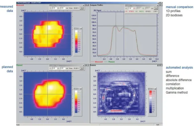
Figure 1: Screenshot of a dose comparison program.

The two images to the left are the measured and calculated doses; the right upper plot contains the profile of the doses while the right lower plot is the gamma comparison image. Red highlights region of disagreement between the two dataset. Source: OmniPro I’mRT documentation

The gamma index is calculated based on a dose difference and distance to agreement criteria and the measured dose data is usually used as the reference.

The gamma value, , for the measurement point is defined as

10

Where

√

| |

and

Where is the dose calculated for a given point, is the dose measured for the calculated point which is often taken as the reference dose, is the defined passing distance between isodose points (the calculated and the measured), is the dose difference value between the calculated and measured which is accepted as pass. For each point in the evaluated data points, the gamma is computed as specified by equation 1.3 and the evaluation is scored. This scoring could be said to be Boolean and is specified as

{

Where 1 and 0 specifies passed and failed evaluation points respectively. The

gamma calculation is performed for all (Low et al., 1998, Rhein and Haring,

2006). In other words, if the dose calculated and that measured does not agree

based on the defined evaluation criteria (distance to agreement and acceptable

11

dose difference values), the calculation for that point fails and vice versa. The

result of gamma analysis is usually presented in terms of the percentage

agreement between calculated and measured points. Hrbacek et. al. reported very

good gamma evaluation results using the OmniPro I'mRT® software in their work

(Hrbacek et. al., 2007), which shows that even at a stringent gamma evaluation

criteria of 1 mm and 1 % for the distance to agreement and dose difference values

respectively, that 70 % of the evaluated profiles had gamma values of less than or

equal to one.

12

2. Materials and methods 2.1 Dose calculation and delivery

Calculation for dose distribution was made using Monaco treatment planning system (Elekta, Monaco Version 2.03.00). The algorithm employs Monte Carlo simulation for dose computation. Multiple calculations were made using variances (dose calculation uncertainty) of 0.5, 1, 2, 3, 5 and 10%. The Monaco® training guide recommends using variance ranging from 1 – 3% although the full available variance treatment planning system ranges from 0.5% - 10%. Calculations were made for various regular square and rectangular open fields, irregular shaped fields and IMRT clinical cases. The calculation times at different variances for some field shapes and sizes were recorded and analyzed.

The calculated dose was exported to the control software of the linear accelerator,

Mosaiq®, and ultimately to the accelerator itself. The linear accelerator is an

Elekta Synergy (Elekta Oncology Systems Ltd, Sweden). A beam energy of 6 MeV

was used for calculation and the same beam energy was used for the exposure of

the dosimetric film. The films used are GAFCHROMIC EBT2 dosimetric films that

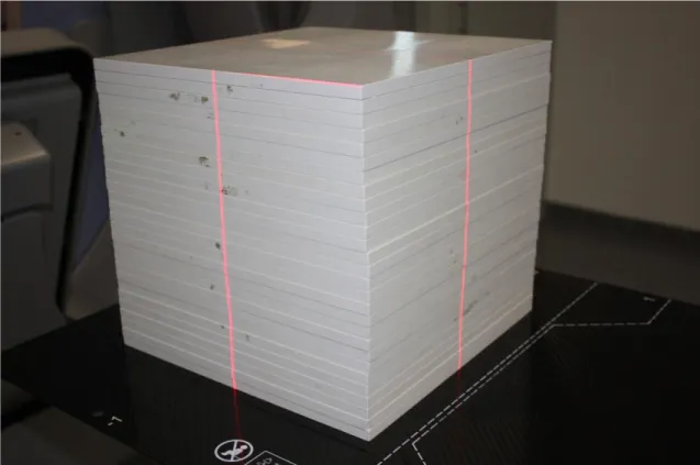
were exposed in a homogenous solid water phantom. The phantom has 29 slabs

each of dimension 30 X 30 X 1 cm and the films were exposed at a chosen depth

corresponding to that specified when the treatment plan was exported from the

treatment planning system to the machine. 100 cm SSD was used for the film

13

exposure. Figures 1 and 2 show the linear accelerator and the solid water phantom used for the dosimetric studies respectively.

Figure 2: An Elekta Synergy linear accelerator

14

2.2 Film calibration, comparison of calculated and measured dose

Prior to exposing the dosimetric films, the films were carefully labeled for proper identification and scanned using EPSON Expression® 10000 XL Photo Scanner and the pre-exposed film images were saved.

Figure 3: The solid water phantom used for film exposure

The films were exposed in the homogenous water phantom and subsequently

processed. The processed films, which contain the measured dosimetric

information were scanned using the same scanner settings and format as was used

for the scanning of the pre-exposed film. The scanning set up employed also

ensured that the pre-exposed and exposed films were scanned using the same

15

orientations. The difference between the pre-exposed and exposed film was subtracted using an algorithm to give the true value of the optical density – the correct measured dose. The subtraction is necessary because the full optical density of the exposed film also include background density due to film fog and the density of the film materials, such as the film base and emulsion layer. An algorithm was used to convert the measured optical density to dose values. The calculated dose was compared with the measured dose using OmniPro I'mRT®

software. The software employs the Gamma evaluation method described in

earlier section. Four dose difference (DD) and distance-to-agreement (DTA) values

were used for the comparison. The values used are 5 % and 5 mm, 4 % and 3 mm,

3 % and 3mm, and 2 % and 2 mm for the DD and DTA pairs respectively.

16

3. Result

3.1 Gamma analysis and computation time

Figure 4 shows the calculated dose distribution for square fields of 10 cm

using

variances of 0.5, 1, 2, 3, 5 and 10%. At low variances, the calculated dose

distribution appears smooth with little noise, whereas at higher variances, the

distribution appears to contain a lot of noise which appears as increase in the

graininess of the image as the variance increases.

17

(A) variance 0.5% (B) variance 1%

(C) variance 2% (D) variance 3%

(E) variance 5% (F) variance 10%

Figure 4: Calculated dose distribution

The figure shows 6 images shows the dose distribution calculated for a square field

using different variance. Note how the graininess (noise) in the images increases

with increasing variance.

18

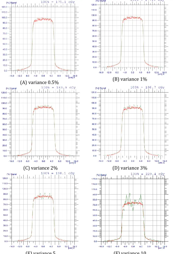
Figure 5 shows the profile of the calculated and the measured dose distribution at

different variances for a square 10 x 10 cm field. The red plots in the figures

represent the profile of the measured dose while the green ones show the profile

of the calculated dose. At low variances, the measured and calculated dose

distributions are mostly similar, whereas at higher variances, the noise in the

calculated dose is increased, evident as the spikes present in the profile.

19

(A) variance 0.5% (B) variance 1%

(C) variance 2% (D) variance 3%

(E) variance 5 (F) variance 10

Figure 5: Profile of calculated and measured dose distribution

Note how the noise which is evident as the spikes in the calculated dose

distribution increases with increasing variance.

20

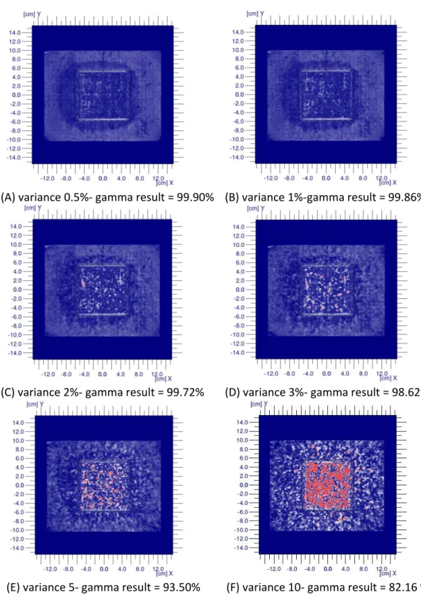
Figure 6 show the gamma evaluation results for dose calculated using different

variance. The gamma comparison was made with DD and DTA of 4 % and 3 mm

respectively. The values of the variance used in calculating the dose are included in

the figure. It can be seen that the gamma result decreases (grainy red regions) as

the variance (uncertainty in calculation) increases due to increasing disagreement

of the data pairs as the variance is increased.

21

(A) variance 0.5%- gamma result = 99.90% (B) variance 1%-gamma result = 99.86%

(C) variance 2%- gamma result = 99.72% (D) variance 3%- gamma result = 98.62%

(E) variance 5- gamma result = 93.50% (F) variance 10- gamma result = 82.16 %

Figure 6: Gamma evaluation result

The gamma evaluation result for the square field shows the decrease in agreement

between the calculated and measured dose distribution as the variance is

increased.

22

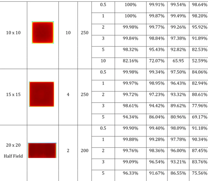
Table 1 shows the field sizes, approximate shape, irradiation parameters (depth, monitor units (MU)), variances, gamma evaluation criteria and results for square fields. For all the fields, variances of 0.5, 1, 2, 3 and 5% were used in calculating the dose distribution while DD and DTA value pairs of 5 % and 5 mm, 4% and 3 mm, 3

% and 3 mm and 2 % and 2 mm were chosen as the pass criteria and used for evaluations. Gamma scores of 95 – 100% are considered as having passed the evaluation whereas lower scores are considered as a failure of agreement between the computed and measured dose distribution. It can be seen that at DD and DTA of 5 % and 5 mm respectively, nearly all the gamma evaluation have results of 100

% and only the evaluation result for the 15 X 15 field made with a variance of 5%

failed the gamma evaluation at the stated DD and DTA values. It can also be seen that generally, the passed results generally reduce as the field size increases. For instance, at DD and DTA of 3 % and 3 mm and field sizes of 1.1 cm

to 3 cm

except for the calculated dose made with a variance of 5%, all gamma evaluation results exceeded the pass value. However, at larger field sizes, the failed points increase.

At low variance up until the 3% recommended and gamma criteria 3 % and 3

mm for the DD and DTA respectively, almost all the calculated dose agrees with the

measured dose, however at higher variance values, the level of agreement is

reduced.

23

Table 1 shows the gamma evaluation result for the square fields studied.

Field Size

x

The Shape Depth

(cm) MU Variance (%)

The Result Of Gamma Index Dose Comparison Tools:

The Dose Difference (DD)

&

The Distance-To-Agreement (DTA)

DD 5% 4% 3% 2%

DTA 5mm 3mm 3mm 2mm

1.1 x 1.1 5 250

0.5 100% 100% 100% 100%

1 100% 100% 100% 100%

2 100% 100% 100% 100%

3 100% 100% 100% 100%

5 100% 100% 100% 100%

2 x 2 5 250

0.5 100% 100% 100% 100%

1 100% 100% 100% 100%

2 100% 99.17% 98.15% 93.87%

3 100% 98.27% 97.15% 91.71%

5 100% 98.00% 97.00% 89.60%

3 x 3 5 250

0.5 100% 99.71% 98.65% 94.59%

1 100% 99.70% 98.83% 93.94%

2 100% 99.93% 98.61% 92.62%

3 100% 99.57% 98.01% 88.94%

5 98.75% 96.71% 94.41% 86.65%

5 x 5 5 250

0.5 100% 100% 99.66% 91.69%

1 100% 99.58% 97.94% 88.02%

2 99.92% 97.29% 94.12% 81.67%

3 99.50% 96.50% 92.88% 78.16%

5 97.93% 93.22% 89.17% 77.25%

24

10 x 10 10 250

0.5 100% 99.91% 99.54% 98.64%

1 100% 99.87% 99.49% 98.20%

2 99.98% 99.77% 99.26% 95.92%

3 99.84% 98.84% 97.38% 91.89%

5 98.32% 95.43% 92.82% 82.53%

10 82.16% 72.07% 65.95 52.59%

15 x 15 4 250

0.5 99.98% 99.34% 97.50% 84.06%

1 99.97% 98.95% 96.43% 82.94%

2 99.72% 97.23% 93.32% 80.61%

3 98.61% 94.42% 89.62% 77.96%

5 94.34% 86.04% 80.96% 69.17%

20 x 20 Half Field

2 200

0.5 99.90% 99.40% 98.09% 91.18%

1 99.88% 99.28% 97.78% 90.34%

2 99.76% 98.36% 96.00% 87.45%

3 99.09% 96.54% 93.21% 83.76%

5 96.33% 91.67% 86.55% 75.56%

Table 2 shows the results for the rectangular fields. For the 10 X 2 cm and 15 X 5

cm fields, note that two measurements were made with the films oriented

horizontally and vertically relative to the positions of the MLCs and the interesting

pattern of the comparison results observed for the two types of orientations. The

gamma results for the 2 X 10 cm films are generally better than the results for the

10 X 2 cm film, whereas the results for the 15 X 5 cm films are generally better

than the results for the 5 X 15 cm film.

25

Table 2 shows the gamma result for rectangular fields

Field Size

The Shape Depth

(cm) MU Variance (%)

The Result Of Gamma Index Dose Comparison Tools:

The Dose Difference (DD) (%)

&

The Distance-To-Agreement(DTA) (mm)

DD 5% 4% 3% 2%

DTA 5 mm 3 mm 3 mm 2 mm 0.6 x 1.1

Smallest Field in Monaco

5 250

0.5 100% 100% 100% 100%

1 100% 100% 100% 100%

2 100% 100% 100% 100%

3 100% 100% 100% 100%

5 100% 100% 100% 100%

10 x 2 5 250

0.5 100% 97.55% 94.16% 76.95%

1 99.97% 97.17% 94.05% 76.35%

2 99.92% 95.51% 91.30% 71.98%

3 99.80% 95.18% 89.87% 70.77%

5 98.40% 90.38% 86.62% 69.57%

2 x 10 5 250

0.5 100% 99.60% 98.81% 89.74%

1 100% 99.58% 98.74% 89.30%

2 99.94% 98.94% 97.10% 87.93%

3 99.51% 97.94% 96.27% 87.77%

5 99.48% 97.61% 96.15% 87.20%

15 x 5 5 250

0.5 99.85% 96.55% 91.59% 74.31%

1 99.62% 96.39% 91.18% 74.00%

2 99.01% 94.60% 89.07% 72.41%

3 98.01% 91.87% 86.67% 71.31%

5 93.58% 85.89% 80.38% 64.19%

5 x 15 5 250

0.5 99.57% 90.49% 78.35% 53.57%

1 98.67% 89.24% 78.08% 52.66%

2 96.67% 85.03% 75.68% 56.69%

3 94.48% 82.79% 74.99% 54.63%

5 88.04% 76.48% 70.88% 57.51%

26

Table 3 shows the gamma evaluation results for irregular fields obtained at

various dose difference (DD) and distance to agreement (DTA) values. As should

be expected, it can be seen that as the variance increases, the gamma evaluation

result (proportion of pass) decreases. At DD and DTA of 3 % and 3 mm

respectively, almost all dose calculation made with variance of less than 5 %

passed the gamma evaluation, whereas most of the calculation made with

variances equal to or higher than this value mostly failed (gamma ≤ 95%) .

27

Table 3 shows the field shape, exposure parameters, gamma criteria and results for irregular fields

The Field The

Shape Depth (cm)

MU Variance (%)

The Result Of Gamma Index Dose Comparison Tools:

The Dose Difference (DD) (%)

&

The Distance-To-Agreement(DTA) (mm)

DD 5% 4% 3% 2%

DTA 5mm 3mm 3mm 2mm

Letter L 5 250

0.5 100% 99.37% 98.54% 90.84%

1 100% 99.21% 98.23% 90.38%

2 100% 98.89% 98.01% 89.84%

3 99.52% 97.75% 96.63% 89.55%

5 99.21% 96.02% 94.38% 83.06%

10 95.91% 89.48% 86.83% 74.50%

Letter E 5 250

0.5 100% 99.00% 97.75% 84.82%

1 100% 98.62% 97.22% 84.31%

2 99.96% 97.20% 95.51% 81.76%

3 99.58% 96.38% 94.33% 82.47%

5 98.31% 93.78% 92.13% 79.18%

10 96.14% 90.63% 88.00% 73.74%

Diamond

Shape 5 250

0.5 98.71% 93.54% 90.65% 78.64%

1 97.95% 93.37% 89.85% 76.92%

2 96.92% 92.24% 89.14% 76.95%

3 96.15% 92.04% 89.30% 78.41%

5 95.91% 90.72% 87.78% 76.01%

10 91.82% 85.76% 81.88% 68.16%

Random

Shape 5 250

0.5 100% 99.12% 98.05% 84.77%

1 100% 99% 98.8% 84.95%

2 99.88% 98.32% 96.19% 82.43%

3 99.30% 96.42% 94.33% 81.35%

5 97.75% 94.26% 91.85% 78.84%

10 92.60% 85.70% 82.26% 67.56%

28

Table 4 presents the Monte Carlo dose calculation time at different variances. The table shows a huge increase in the calculation time as the uncertainty is reduced.

The calculation time appears to increase exponentially as the variance is reduced.

Table 4 Calculation times for square fields at different variances

Figure 7 shows calculation time plotted against variance for some field size which shows that the time increase with reduction in variance does indeed appear to be exponential. The calculation time increased as the variance is reduced and as the field size is increased.

Calculation time (s)

Variance (%) 2cm

3cm

5cm

7cm

10cm

15cm

20cm

0.5 % 41,5 69 163 306 621 1363 2412

1 % 25,7 34 57 94 174 368 632,5

2 % 22,5 25 31,5 39,5 62,2 119 192

3 % 21,5 23,5 25,5 31 40,5 71,5 113

5 % 20 22,5 23,5 25 30,7 47.5 69

29

Figure 7: Plot showing Monte Carlo calculation time as a function of variance and field size

Depence calculation time on variance at different field sizes

0 2

4 0 6

50 100

Field size = 2 cm ²

Variance [%]

T im e [ s ]

Data

interpolation 0 2

4 0 6

50 100

Field size = 3 cm ²

Variance [%]

T im e [ s ]

0 2

4 0 6

100 200

Field size = 5 cm ²

Variance [%]

T im e [ s ]

0 2

4 0 6

200 400

Field size = 7 cm ²

Variance [%]

T im e [ s ]

0 2

4 0 6

500 1000

Field size = 10 cm ²

Variance [%]

T im e [ s ]

0 2

4 0 6

1000 2000

Field size = 15 cm ²

Variance [%]

T im e [ s ]

0 2

4 0 6

2000 4000

Field size = 20 cm ²

Variance [%]

T im e [ s ]

30

3.2 Dosimetric effect of variance on DVH – IMRT clinical cases

Figures 8 and 9 are used to show the effect of using different variance when computing the dose distribution in a patient. Considering figure 8, the calculation made with a variance of 10 % appears to agree more with that made with a variance of 0.5 % (assumed to be the most correct), than the calculation made with a variance of 5 %. In the region of the dose to about 10 % of the structures (high dose region), the effect of varying variance seems to be most evident with about 1000 cGy difference in the dose to the structure in this region being projected with the dose calculations made with variance of 0.5, 1 and 3 % and that made with a variance of 5 %.

Figure 8 shows the effect of using different variance in computing the dose on the dose volume histogram (DVH) of a patient (case 1)

0 1000 2000 3000 4000 5000 6000 7000 8000 9000 0

10 20 30 40 50 60 70 80 90 100

Dose [cGy]

Volume [%]

Effect of varying variance on DVH

Variance: 0.5%

Variance: 1%

Variance: 2%

Variance: 3%

Variance: 5%

Variance: 10%

31

Considering figure 9, if the DVH computed with a variance of 0.5 % is assumed to be the most accurate, then the observed pattern is mostly in agreement with the expectation since that made with a variance of 10 % deviated the most from this value as is expected, and that computed with a variance of 1 % is probably the second most accurate (again, assuming that that made with a variance of 0.5 % will agree more with the measured. No measurements were made in the case of the patient dose calculation data.

Figure 9: shows the effect of using different variance in computing the dose on the DVH of a patient (case 2).

0 1000 2000 3000 4000 5000 6000 7000

0 10 20 30 40 50 60 70 80 90 100

Dose [cGy]

Volume [%]

Effect of varying variance on DVH

Variance: 0.5%

Variance: 1%

Variance: 2%

Variance: 3%

Variance: 5%

Variance: 10%

32

4. Discussion

Table 3 shows the dose calculation time for a square 10 X 10 cm field while tables 1 and 2 show the gamma evaluation results. From table 1, it can be seen that the gamma evaluation results for the calculations made with variances of 0.5 and 1 % are quite similar. Table 3 however show the dose calculation time with a variance of 0.5% is more than 3 times the time required for dose calculation with an uncertainty of 1%. It can thus be concluded that there is no significant gain in going lower than a variance of 1% since there is no significant improvement in the accuracy of the calculated dose when compared with the measured. Figure 7, which is a plot of the computation time against variance show that it will be impossible to achieve a Monte Carlo calculation dose distribution calculation of absolute accuracy, i.e. one with no variance. This is so because as the plots clearly show, as the variance tends to zero, the computation time tends to infinity.

The recommended upper and lower values for variance to be used for calculation

of dose distribution are 3 % and 1 % respectively. The findings of this research

also agrees with the suggestion since at higher variances, the result of the gamma

result is decreased due to increase failure of agreement between the calculated

and the measured dose distribution. The results of this research is in agreement

with the recommended variance values of 1% to 3% since the range of values

appear to be very good compromise between reducing calculation time and

having an accurate calculation of dose distribution. Based on the gamma result, at

33

DD of 4% and DTA of 3 mm, there is agreement between the calculated and measured dose distribution in almost all the cases. This value is also the recommended value that is used in clinical routine for IMRT quality assurance. The purpose of the dose computation in the first place is to accurately determine the dose that will be deposited in the patient from the beam geometry employed for the treatment. To simulate the dosimetric impact due to the use of different variance values in the dose computation, patient dose was computed for IMRT cases using different variance values. The results showed substantial difference between the plans made with the different variances (Figures 8 and 9). Dose computed with variances of 1 and 10 % for a subject showed up to 1000 cGy difference in the dose to 90 % of the structure’s volume, while the dose calculated with variance of 0.5 and 5 % for another subject showed up to 1000 cGy difference in the dose to approximately 10 % volume of the structure. Such large variation could lead to adverse effects (Indrin et. al., 2007)..

The results also show that at small field sizes, the calculated and measured dose distribution always agrees irrespective of the variance values used. In other words, for small field size, even when high values of variance were used during the dose calculation, the gamma evaluation passed. Thus for a small field, large uncertainties in calculation still yielded accurate result. This means that when the field is small, the large variances can be employed to reduce the calculation time.

At DD and DTA of 5% and 5 mm respectively, the evaluation result is nearly passed

in all the cases. However, this is not a good evaluation criterion since the pass

criterion is fairly loose and a dose difference value of 5% between the calculated

34

and predicted is substantial. Lower values such as the 4% and 3 mm values commonly employed in QA programs are more stringent criteria that should be used.

A unique pattern is observed for the gamma evaluation result of the rectangular field (Table 2). The 10 x 2 cm and 2 x 10 cm field sizes are of the same dimension;

however both shapes are defined by different number of MLC leaf pairs that has to

be in the open position during the irradiation of the film. For the 10 x 2 cm field

size, only2 leaf pairs are open, whereas the 2 x 10 cm fields requires 10 MLC leaf

pairs to be in the open position ( leaf width = 1 cm). The 10 x 2 cm field will be

referred to as the horizontally oriented field and the 2 x 10 cm field will be

referred to as the vertically oriented field. Both field dimensions will be referred to

as case a. The same convention will be used in describing the 15 x 5 cm and 5 x 15

cm fields, i.e. 15 x 5 cm field being horizontally oriented and 5 x 15 cm field being

vertically oriented. Both fields will be referred to as case b. It was observed that

the gamma results for the vertically oriented field was better than that of the

horizontally oriented field for all observations in case a, with a reversal of the

pattern in case b, i.e. the horizontally oriented field having more pass values than

the vertically oriented one. The reason for such discrepancies and reversal of

pattern is not easily understandable. This observation is however, not statistical

since this pattern was true for all 40 comparison points made for the two field

sizes.

35

The results of this research are also mostly in agreement with results reported by

earlier researchers. At a variance of 3 % and gamma evaluation criteria of 3 % and

3 mm for the DD and DTA respectively, the results are mostly similar with that

reported by Wang (Wang et al., 1996). However, with an increase in the acceptable

variance in dose calculation to 5 %, the result agree more with that reported in the

work of Ma (Ma et al., 2000, Oldham and Webb, 1997). From the results, it can thus

be possible to predict the calculation time (for a square field in this case) for any

given field size and variance with fair degree of accuracy with increase with

increasing field size. Since the data shows calculated time to tend more towards

agreeing with the modeling function as the field size increases. The results also

show that the calculation times tend to infinity as the variance approaches zero.

36

5. Conclusion

In conclusion, the result of this work showed the Monte Carlo method to achieve

good dose calculation results. The results are similar to that reported in previous

literature. However, the accuracy of the dose calculation comes at the expense of

computation time whose increase appears exponential with increasing dose

calculation accuracy. The dosimetric effect of using different variances on the DVH

pattern was studied and the result showed substantial dose difference between

dose computations made with low and high variances. This huge dose difference

due to variance selection could result in serious therapeutic consequences.

37

References

BIELAJEW, A. 2007. The Monte Carlo Simulation of Radiation Transport In: MAYLES, P., NAHUM, A. & ROSENWALD, J. C. (eds.) Handbook of Radiotherapy Physics Theory and Practice. Florida: Taylor & Francis Group. pp 75 - 87.

FIPPEL, M. 2006. Monte Carlo Dose Calculation for Treatment Planning. In: SCHLEGEL, W., BORTFELD, T. & GROSU, A.-L. (eds.) New Technologies in Radiation Oncology Medical Radiology. Heidelberg: Springer. pp 197 - 206.

HOGSTROM, K. R., MILLS, M. D. & ALMOND, P. R. 1981. Electron beam dose calculations.

Phys Med Biol 26, 445 – 459

HRBACEK J., DEPUYDT T., NULENS A., SWINNEN A., VAN DEN HEUVE F. 2007.

Quantitative evaluation of a beam-matching procedure using one- dimensional gamma analysis. Med. Phys. 34 (7), 2917 - 2927

INDRIN J. CHETTY, BRUCE CURRAN, JOANNA E. CYGLER, JOHN J. DEMARCO, GARY EZZELL, BRUCE A. FADDEGON, IWAN KAWRAKOW, PAUL J. KEALL, HELEN LIU, C.-M. CHARLIE MA, D. W. O. ROGERS, JAN SEUNTJENS, DARYOUSH SHEIKH- BAGHERI & JEFFREY V. SIEBERS. 2007. Report of the AAPM Task Group No. 105:

Issues associated with clinical implementation of Monte Carlo-based photon and electron external beam treatment planning. Med. Phys. 34 (12), 4818 – 4853.

JENGHWA CHANG, GIKAS S. MAGERAS, CHEN S. CHUI, CLIFTON C. LING & LUTZ, W. 2000.

Relative Profile And Dose Verification Of Intensity-Modulated Radiation Therapy Int. J. Radiation Oncology Biol. Phys., 47, 231– 240.

KAWRAKOW, I., FIPPEL, M. 2000. Investigation of variance reduction techniques for Monte Carlo photon dose calculation using XVMC. Phys. Med. Biol. 45, 2163 – 2184

KAWRAKOW I., ROGERS D. W. O., & WALTERS B. R. B. 2004. Large efficiency improvements in BEAMnrc using directional bremsstrahlung splitting. Med. Phys.

31, 2883–2898.

LOW, D. A., HARMS, W. B., MUTIC, S. & PURDY, J. A. 1998. A technique for the quantitative evaluation of dose distributions Med. Phys., 25, 656 - 661.

MA, C.-M., PAWLICKI, T., JIANG, S. B., LI, J. S., DENG, J., MOK, E., KAPUR, A., XING, L., MA, L. &

BOYER, A. 2000. Monte Carlo verification of IMRT dose distributions from a commercial treatment planning optimization system. Phys. Med. Biol, 45, 2483–

2495.

38

MACKIE, R. T., LIU, H. H. & MCCULLOUGH, E. C. 2007. Treatment Planning Algorithms:

Model-based Photon Dose Calculations. In: KAHN, F. M. (ed.) Treatment Planning in Radiation Oncology. 2 ed.: Lippincott Williams & Wilkins.

MACKIE, T. R., RECKWERDT, P., MCNUTT, T., GEHRING, M. & SANDERS, C. (eds.) 1996.

Photon beam dose calculations Teletherapy: Present and Future, Madison, WI:

Advanced Medical Publishing.

MACKIE, T. R., SCRIMGER, J. W. & BATTISTA, J. J. 1985. A convolution method of calculating dose for 15 MV X-ray. . Med Phys, 12, 188–197

MOHAN, R., CHUI, C. S. & LIDOFSKY, L. 1986. Differential pencil beam dose computation model for photons Med. Phys, 13, 64– 73

Monaco®. Introduction to Monaco IMRT. Monaco® Training Guide.2008

NAHUM, A. 2007. Monte-Carlo Based Patient Dose Computation. In: Mayles P, Nahum, A, Rosenwald, J.C (eds.). Handbook of Radiotherapy Physics Theory and Practice. Florida: Taylor & Francis Group. pp 603 - 631.

OELFKE, U. & SCHOLZ, C. 2006. Dose Calculation Algorithms In: SCHLEGEL, W., BORTFELD, T. & GROSU, A.-L. (eds.) New Technologies in Radiation Oncology Heidelberg: Springer. pp 187 - 196

OLDHAM, M. & WEBB, S. 1997. Intensity-modulated radiotherapy by means of static tomotherapy: a planning and verification study Med. Phys. , 24 827–36.

Podgorsak, E. B. 2005. External beams: Physical aspect In: Podgorsak, E. B. (ed.) Radiation Oncology Physics: A Handbook for Teachers and Students. IAEA. Vienna, 2005. pp 161 - 217

RHEIN, B. & HARING, P. 2006. 3D Quality Assurance Systems. In: SCHLEGEL, W., BORTFELD, T. & GROSU, A.-L. (eds.) New Technologies in Radiation Oncology Heidelberg: Springer.

ROGERS D. W. O., FADDEGON B. A., DING G. X., MA C. M., WE J., & T.R. MACKIE. 1995.

BEAM: A Monte Carlo code to simulate radiotherapy treatment units, Med. Phys.

22, 503–524.

ROSENWALD, J.-C. 2007. Principles of Patient Dose Computation. In: MAYLES, P., NAHUM, A. & ROSENWALD, J. C. (eds.) Handbook of Radiotherapy Physics Theory and Practice. Florida: Taylor & Francis Group.

WANG, X., SPIROU, S., LOSASSO, T., STEIN, J., CHUI, C. & MOHAN, R. 1996. Dosimetric

verification of intensity modulated fields Med. Phys., 23 317–28.