submitted in partial fulfillment of the requirements for the degree of

(1)

Max Planck Institute for Physics Fakult¨ at f¨ ur Physik Technische Universit¨ at M¨ unchen

A thesis

submitted in partial fulfillment of the requirements for the degree of

Master of Science

in

Nuclear, Particle and Astrophysics

Bayesian Analysis of the First Data of the KATRIN Experiment

Martin Ha Minh

October 30, 2018

Supervisor: Prof. Dr. Susanne Mertens

(2)

(3)

Abstract

Neutrino oscillations prove that neutrinos have a mass and provide a means to de- termine the squared mass di↵erence between neutrino mass eigenstates. However, their absolute mass scale is still unknown. A neutrino mass model independent approach to measure the absolute neutrinos mass scale is based on the kinematics of the b-decay. The Mainz and Troitsk neutrino mass experiments currently provide the best upper limit on the e↵ective electron antineutrino mass of 2 eV/c ² .

The KArlsruhe TRItium Neutrino (KATRIN) Experiment is designed to improve the sensitivity by one order of magnitude to 200 meV/c ² (90% C.L.). It investigates the tritium b-decay close to the kinematic endpoint of the energy spectrum with a high-resolution electrostatic spectrometer ( E = 0.93 eV at 18.6 keV).

This thesis is focused on the analysis of two data sets: (1) from a calibration campaign using the full beamline in summer 2018 using a gaseous ^83m Kr source and (2) from our first measurement using gaseous tritium in spring 2017, setting the final preparations for the neutrino mass measurement campaign next year.

In this work we investigate the usage of the powerful Bayesian Analysis Toolkit (BAT),

which was developed at the Max-Planck-Institute for Physics. In particular our studies

focus on the aspect of, firstly, how to combine the data of di↵erent pixels of the 148 channel

focal plane detector, and secondly, how to include systematic uncertainties in the fit using

the Bayesian school of data analysis. We also compare di↵erent priors and their influence

on our model selection. As a result, we demonstrate a very good agreement of the model

and the data and in particular we establish the applicability of BAT for the KATRIN data

analysis.

(4)

(5)

Neutrino Physics

First, we want to shortly illustrate the history of the neutrino. We recount the postulation and discovery of the neutrino and its di↵erent flavors. Next, we depict the journey of neutrino oscillation studies and the proof of the existence of the neutrino mass. We also compile methods for determining the absolute mass of the neutrino.

1.1 Postulation and Discovery of Neutrino

The neutrino was first proposed by Wolfgang Pauli [Pau] in 1930. Considering the knowl- edge at that time, the b-decay seemed to be violating multiple conservation laws; e.g.

for the assumed two-body decay, a fixed energy for the beta electron would be expected;

instead a continuous energy spectrum was observed. Pauli postulated the neutrino, that would be emitted alongside with the electron and hence share the decay energy. Later, Enrico Fermi published his work Theory of b-decay in 1934 where he formulated the decay involving the neutrino and lent it its name [Fer34].

In 1956 the neutrino, specifically the electron antineutrino, was finally proven to exist by Cowan and Reines with an approach using inverse b-decay [Cow+56]. Subsequent experiments also showed that other neutrino flavors exist: the muon neutrino by Schwartz, Ledermann, and Steinberger in 1962 [Dan+62] and the tau neutrino by the DONUT experiment in 2000 [Kod+01].

1.2 Neutrino Oscillations

The Homestake experiment [DHH68] [Cle+98] in the 1970s discovered the solar neutrino problem: compared to the expected flux of electron neutrinos from the sun, they could only detect a fraction of that. Many other experiments confirmed the same problem.

Pontecorvo earlier, along with his theoretical description of the neutrino mass and flavor

eigenstates, predicted a mechanism with which neutrinos could change their flavors based

(8)

on their energy and distance traveled, the neutrino oscillation [Pon58]:

The mass eigenstate of the neutrino is a superposition state of the flavor eigenstates and vice-versa:

| ⌫ i i = X

↵

U ↵i | ⌫ ↵ i ,

| ⌫ _↵ i = X

i

U _↵i ^⇤ | ⌫ _i i . (1.1)

Where | ⌫ _i i and | ⌫ _↵ i are neutrino mass and flavor eigenstates respectively, and U _↵i and U _↵i ^⇤ are the Pontecorvo–Maki–Nakagawa–Sakata matrix elements [MNS62] and their complex conjugates. And for the propagation of a mass eigenstate:

| ⌫ _i (t) i = e ^iE

ⁱ

^t | ⌫ _i i . (1.2) The probability for a flavor state transition is then:

P _↵ _! = h ⌫ (t) | ⌫ _↵ i = X

i,j

U _↵i ^⇤ U _i U _↵j U ^⇤ _j exp

✓

i m ² _ij L 2E

◆ , (1.3)

where m ² _ij = m ² _i m ² _j is the squared neutrino mass di↵erence, L is the distance traveled by the neutrino, and E is its energy. This means for neutrino oscillations to occur, at least one mass eigenvalue has to be di↵erent from the others, and cosequently, at least one mass eigenvalue has to be non-zero.

Super-Kamiokande [Hos+06] and the SNO experiment [Ahm+01] later demonstrated the existence of neutrino oscillations, and e↵ectively showed that neutrinos need to have a mass. Many experiments afterwards studied neutrino oscillations and their parameters.

However from neutrino oscillations we can only deduce the mixing angles as well as the mass squared di↵erences, but not the absolute mass scale and their ordering.

1.3 Determining the Absolute Neutrino Mass

For the measurement of the absolute neutrino mass scale, di↵erent approaches exist. We present a non-exhaustive list with a short description of their methods.

1.3.1 Cosmology

The LCDM is the cosmological model that describes the universe according to the Big

Bang. Based on the cosmic microwave background data combined with large-scale struc-

ture formation observations the neutrino mass can be deduced. The imprint of a neutrino

mass on these cosmological probes is based on the fact that neutrinos act as hot dark

matter and thus wash out small scales structures in our cosmos. The Planck observations

(9)

set the limit of the neutrino mass eigenstate sum to P

i m _i < 0.23 eV [P A+16]. This approach is however highly model dependent.

1.3.2 Neutrinoless Double Beta Decay

A property that is still unknown about the neutrino is whether it is a Dirac or a Majorana particle, the latter implying it is its own antiparticle. A Majorana neutrino would allow the so-called neutrinoless double beta decay:

(A, Z) ! (A, Z + 2) + 2e (1.4)

In the decay spectrum of the electron energies this would manifest itself in a sharp peak at the Q-value of the decay. The decay rate of this mechanism is proportional to the e↵ective Majorana mass of the electron neutrino m :

0⌫ = G | M | ² | m | ² (1.5)

With G the two-body phase-space factor and M the nuclear matrix element. The most stringent limit on the e↵ective Majorana mass at the moment is set by the KamLAND- Zen experiment with upper limits in the range of 61 – 165 meV [Gan+16]. This approach makes the assumption however that the neutrino is indeed a Majorana particle; in addition the nuclear matrix element is accompanied by a large uncertainty.

1.3.3 Tritium Beta Decay

A neutrino mass model independent approach to determine the absolute neutrino mass is the measurement of the kinematics of the -decay near the endpoint. A massive neutrino, no matter how small its mass, leaves a small shape distortion in the spectrum that can be measured:

d

dE / X

i

| U _ei | ² q

E _⌫ ² m ² _i (1.6)

Equation (1.6) shows the relation of the neutrino mass eigenstates m i with the b-decay.

We will discuss it in detail in section 6.1. By accurately measuring the spectrum, it is possible to make statements about the e↵ective electron neutrino mass m _⌫ = P

i | U _ei | ² m _i . Using this approach, the Mainz [Kra+05] and Troitsk [Ase+11] neutrino mass experiments have set the upper limit of the e↵ective electron antineutrino mass to 2 eV/c ² [Tan+18].

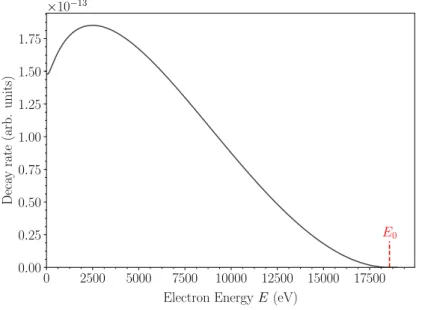
This is also the method the KATRIN experiment pursues. Fig. 1.1 shows the b-decay

spectrum and fig. 1.2 shows the signature of di↵erent e↵ective electron neutrino masses.

(10)

0 2500 5000 7500 10000 12500 15000 17500 Electron Energy E (eV)

0.00 0.25 0.50 0.75 1.00 1.25 1.50 1.75

Deca y rate (arb. units)

10

¹³

E

0

Figure 1.1: b-decay spectrum with the endpoint E ₀ , i.e. the maximum energy a beta electron can assume with m ⌫ = 0.

1.4 1.2 1.0 0.8 0.6 0.4 0.2 0.0

E E

0

(eV) 0.0

0.5 1.0 1.5 2.0 2.5 3.0 3.5 4.0

Deca y rate (arb. units)

10

²¹

m = 0 eV m = 200 meV m = 1 eV

Figure 1.2: Zoom into the endpoint region of b-decay spectra for di↵erent e↵ective electron

neutrino masses m _⌫ for c = 1.

(11)

Chapter 2

The KATRIN Experiment

The KArlsruhe TRItium Neutrino (KATRIN) Experiment is designed to improve the sensi- tivity of the e↵ective electron antineutrino mass by one order of magnitude to 200 meV/c ² (90% C.L.). It investigates the tritium b-decay close to the kinematic endpoint of the en- ergy spectrum with the combination of a high luminosity gaseous tritium source and a high-resolution electrostatic spectrometer [KK05].

2.1 Experimental Setup

In the following an overview of the most important parts of the KATRIN experiment and their function in the setup is displayed. Fig. 2.1 shows a schematic view of the experimental setup.

Rear Section The rear section [Bab14] is located at one end of the KATRIN experimen- tal setup. A gold plated rear wall defines the starting electrical potential for the electrons.

(1) (2) (3a) (3b) (4a) (4b) (5)

Figure 2.1: A schematic view of the KATRIN experimental setup. The shown elements

are (1) the rear section, (2) the Windowless Gaseous Tritium Source (WGTS), (3a) the

Di↵erential Pumping Section and (3b) the Cryogenic Pumping Section, (4a) the Pre-

Spectrometer and (4b) the Main Spectrometer, and (5) the detector section.

(12)

Additionally it is equipped with monitoring and calibration tools, such as an electron gun for the measurement of the electron energy loss function [Beh+17].

Windowless Gaseous Tritium Source The 10 m long Windowless Gaseous Tritium Source (WGTS) [Ha17] contains the tritium for the experimental analysis. The name stems from its design; windows would increase the electron scattering greatly, which, in this design, is eliminated. The tritium gas in the source is composed of its isotopologues T ₂ , DT and HT; however the main component is T ₂ with a purity of 95%. The tritium produces approximately 10 ¹¹ decays per second, which has to be kept at a relative stability of 10 ³ per hour. The WGTS is therefore equipped with tritium loops, which extract, clean, and reintroduce the gas continuously. The source is operated at a temperature of 30 K and a target column density of 5 · 10 ¹⁷ cm ² .

Transport Section The tritium gas has to be removed before entering the spectrometer section to reduce contamination and background. This happens in the transport section, comprised of two pumping systems: the Di↵erential Pumping Section (DPS) and the Cryogenic Pumping Section (CPS).

The DPS [Luo+06] [Luk+12] is equipped with four turbomolecular pumps to reduce the tritium flow initially by a factor of 10 ⁵ . Additionally, five superconducting magnets at 5.6 T guide the electrons through the beam tube. These are tilted at angles so that the tritium molecules cannot travel in a straight line through the setup.

The CPS [Gil+10] reduces the tritium flow by another factor of 10 ⁷ . Similarly to the DPS, the CPS has seven superconducting magnets to guide the electrons from the source through the kinked beam line. The beam tubes are covered with argon frost at 4 K where the tritium gas condenses. As the molecules accumulate, the frost layer has to be replaced regularly by heating and flushing the section.

Spectrometer Section The spectrometer section is comprised of two spectrometers, the pre-spectrometer and the main spectrometer. Both work under the MAC-E filter (Magnetic Adiabatic Colllimation with Electrostatic filter) principle [LS85][Pic+92]. We discuss this further in section 2.2.1. Additionally they operate under ultra-high-vacuum with < 10 ¹⁰ mbar to reduce electron scattering inside.

The role of the pre-sprectrometer [FW03] [Bor06] is to pre-filter electrons before they enter the main spectrometer. In the neutrino mass measurement the information is con- tained in the spectrum of electrons with an energy close to the endpoint. Electrons below that threshold can be filtered out. These electrons could otherwise ionize residual gas in the main spectrometer and consequently produce additional background, so it is desirable for them to be filtered before.

The main analysis happens in the 23 m long and 10 m wide main spectrometer [Val06].

Depending on the set high voltage the electrons either pass the potential barrier or get

(13)

reflected and lost. By setting the spectrometer to di↵erent voltages and observing the electron rate, the integral b-spectrum is recorded.

Detector Section The Focal Plane Detector (FPD) [Ams+15] counts the electrons that pass the experimental setup. It is a silicon based PIN diode detector with a dead layer of 100 nm, a radius of 4.5 cm, and is segmented in 148 pixels of equal area.

The detector section exhibits many features to maximize the signal from the b-decay electrons. Although mostly used as a counting detector, it also has an energy resolution of 1.4 keV at Full Width Half Maximum (FWHM). This can be used to apply energy cuts to reject background counts. It is additionally cooled down to 30 C to reduce electrical noise. Both passive and active shielding minimize the impact from cosmic rays or surrounding radioactivity. Lastly, a post acceleration electrode in front of the detector accelerates the electrons coming from the main spectrometer.

The pixelation allows for the localization of the measured counts. We can simulate which electrons travel which parts of the experiment and arrive on which pixel. Based on their trajectory the electrons experience slightly di↵erent electromagnetic fields. We take this into account by applying field maps, which we obtain by the particle tracking simulation software Kassiopeia [Fur+17].

2.2 Modelling the Response Function

An electron that is emitted from the source with an energy E can, with a certain proba- bility, pass the experiment and get detected at the end. This probability is described by the so-called response function R. The di↵erential spectrum S with which the electrons are emitted is then observed as the integrated spectrum I:

I(qU) = Z ₊₁

1 S(E) · R(E, qU ) dE. (2.1) I(qU ) denotes the count rate at the retarding potential qU . For a perfect high energy pass filter, the response function would be a Heaviside step function at the retarding potential qU . However due to physical limitations, the response function must be expressed di↵erently. This is discussed in this section.

2.2.1 MAC-E Filter Spectroscopy

The main spectrometer exploits the MAC-E filter principle: Two solenoid magnets at each side of the spectrometer form an axially symmetric inhomogeneous magnetic field.

Electrons are emitted and enter from one end. The magnetic field lines then guide them

into the spectrometer in a cyclotronic motion. On the way from the entrance to the

center, the magnetic field drops by a factor of 20000. This leads to a transformation of the

(14)

perpendicular momentum component into the parallel one. As the change of the magnetic field during one cyclotron revolution is small, this transformation can be seen as adiabatic;

therefore the magnetic moment µ is constant:

µ = ( + 1) · E _?

B = const, (2.2)

for the transverse kinetic energy E, the magnetic field B and the relativistic gamma factor

= E/m e + 1. Inside the spectrometer, an electric field with the voltage U is applied. Its maximum value is at the center of the spectrometer, which coincides with the minimum magnetic field B _A . This central plane is called the analyzing plane. There, almost all of the kinetic energy of the electron is transformed into the parallel component, which is used to overcome the electric potential barrier. Electrons with a parallel kinetic energy higher than qU pass the electrostatic barrier, get reaccelerated, and focused onto the detector.

Electrons with a lower parallel kinetic energy are reflected and generally lost.

From eq. (2.2) we obtain the relative energy resolution of the MAC-E filter:

E

E = B _A

B _max · + 1

2 ( = 0.93 eV at 18.6 keV design value). (2.3) The MAC-E filter can in principle collect and analyze all electrons emitted into a 2⇡

solid angle. However, electrons with large emission angles exhibit large travel distances and therefore have a higher scattering probability inside the source. To minimize this e↵ect, only electrons with an emission angle smaller than the acceptance angle ✓ _max may enter the spectrometer. This is achieved by surrounding the source with a magnetic field B _S < B _max . The maximum acceptance angle is then:

✓ _max = arcsin r B _S

B _max (= 51 design value). (2.4) The transmission function for an ideal MAC-E filter with an isotropically emitting electron source and maximum acceptance angle ✓ _max is then given by:

T (E, qU ) = 8 >

> >

<

> >

> :

0 for E qU < 0,

1 r

1

^E_E^qU ^BS

BA

·

₊₁²

1 q

1

_B^BS

max

for 0  E qU  E,

1 otherwise.

(2.5)

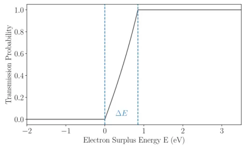
Fig. 2.2 plots an example of the transmission function.

2.2.2 Energy Loss and Response Function

Electrons lose energy by scattering on the gas molecules in the source. This e↵ect has to be

taken into account to accurately describe which electrons pass the filter. The energy loss

(15)

2 1 0 1 2 3 Electron Surplus Energy E (eV)

0.0 0.2 0.4 0.6 0.8 1.0

T ransmission Probabilit y

E

Figure 2.2: An example for the transmission function of a MAC-E Filter set at the retard- ing potential qU = 18500 eV using the KATRIN design values. Additionally the energy resolution E = 0.93 eV is shown.

function f(✏) describes with which probability the electron loses the energy ✏ [Ase+00]:

f(✏) = 1

· d

d✏ , (2.6)

where is the inelastic cross section.

The electron can scatter multiple times while traveling in the source. For n-fold scat- tering the transmission function is convolved with the energy loss function n times. The contribution from each scattering is weighed by the scattering probabilities P _n .

We can then express the response function as follows:

R(E, qU ) = P ₀ · T (E, qU ) ⇤ (✏)+

P ₁ · T (E, qU ) ⇤ f (✏)+

P ₂ · T (E, qU ) ⇤ f (✏) ⇤ f (✏) . . .

= T(E, qU ) ⇤

n X

max

i=0

P _n f _n (✏),

(2.7)

where P _i and f _i (✏) are the respective probabilities and energy loss functions for the

i-th scattering. n _max describes the maximum number of scattering we consider for the

generation of our model. It is usually between 5 and 10, as the probabilities for higher

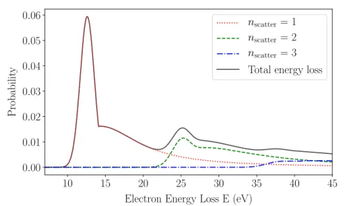
scatterings become negligible. Fig. 2.3 plots the contribution from the energy loss and

fig. 2.4 shows an example of the response function.

(16)

10 15 20 25 30 35 40 45 Electron Energy Loss E (eV)

0.00 0.01 0.02 0.03 0.04 0.05 0.06

Probabilit y

n scatter = 1 n scatter = 2 n scatter = 3 Total energy loss

Figure 2.3: Energy loss contribution from the first four scatterings.

5 0 5 10 15 20 25 30 35

Electron Surplus Energy E (eV) 0.0

0.2 0.4 0.6 0.8

T ransmission Probabilit y

Figure 2.4: The response function for the KATRIN experiment with design values set at

the retarding potential qU = 18500 eV in the range of the first two electron scatterings.

(17)

2.2.3 Run Taking

Measuring Time Distribution The scanning procedure of a run can be expressed by the measuring time distribution (MTD). It describes how much time is spent measuring counts at which retarding potentials. The simplest MTD is the so-called flat MTD which measures the spectrum at equidistant retarding potentials for equal durations.

Run Summary The information about the experiment during one run is called run

summary. It includes the experimental measurements, such as counts and measuring time,

as well as the slow control parameters of the setup, provided by the monitoring facilities

such as the Laser Raman system [Sch+13] or the forward beam monitor [Ell+17].

(18)

Chapter 3

Statistics

This chapter outlines the statistical methods used in this work. Core of the approach is the Bayesian school of analysis on which we also give a short introduction here.

3.1 Choice of Likelihood

The likelihood describes the conditional density of the data given the model expectation.

Since we expect the electrons to arrive at a certain rate at the detector and the events are independent of each other, we choose the Poisson distribution as the probability distribu- tion function describing our spectrum counts in the likelihood function for our analysis.

3.2 Bayesian School of Analysis

The essence of Bayesian statistics is to update a prior knowledge with acquired data to obtain posterior knowledge. This is implied in Bayes’ theorem:

P (✓ | D) = P (D | ✓)P (✓)

R P (D | ✓)P (✓) d✓ , (3.1)

where ✓ is the vector of parameters of a model and D is the data measured by an experi- ment. P (✓ | D) is the so-called posterior probability function that describes the probability distribution assigned to a set of parameters given a set of data. P(D | ✓) is the probability of a set of data given set of parameters, also known as the likelihood.

Prior Probability Distribution P (✓) is the so-called prior probability distribution. It

can describe any prior knowledge of the system, such as theoretical constraints, measure-

ments of systematic parameters, or experimental results. In this case it would be called an

informative prior. It is also possible to use a non-informative prior; the most commonly

used is a constant distribution, also known as the flat prior.

(19)

Posterior Probability Distribution From eq. (3.1) we then obtain the posterior prob- ability distribution by sampling the posterior space. This is the full result of the Bayesian analysis. We can then marginalize our parameters of interest, i.e. integrate over the nui- sance parameters ⌫:

P (✓ | D) = Z

P (✓, ⌫ | D) d⌫. (3.2)

In other words, we sum over all possible nuisance parameter sets, weighted by their proba- bility, to obtain the posterior distribution on our parameter of interest. We can then infer values and uncertainties of our parameters of interest directly from the marginal posterior distributions. We will favor the 95% credible intervals (CI) and the posterior mean, i.e.

the mean values of the marginalized posterior distributions for each fit parameter. The corner.py package [For16] is used for visualization.

Treatment of Systematic Uncertainties In the Bayesian framework the treatment of systematic uncertainties is very straightforward. We can introduce a parameter that describes the systematic uncertainty and apply a prior characterizing its behavior, e.g. a Gaussian function with a mean and width corresponding to the expected values. When marginalizing for the physical parameters, the impact of the systematic parameters will manifest themselves in the posterior distributions.

Bayes Factor The role of the integral in the denominator is to normalize the posterior.

It is also known as the evidence Z , or marginal likelihood. For the mere inference of parameters its calculation is not necessary, however it is practical for comparing models.

Via the posterior odds O:

O = P (M ₁ | D)

P (M ₂ | D) = P (D | M ₁ )

P (D | M ₂ ) · P (M ₁ )

P (M ₂ ) , (3.3)

where P (M 1 ) and P (M 2 ) are the prior probabilities for model M 1 and model M 2 respec- tively. We then make model comparisons based on O. The prior odds ^P _P ^(M _(M

¹

⁾

2

) describe how much credence we lend to each model a priori. Often times we do not prefer any model;

then the posterior odds reduce to the first ratio, called the Bayes Factor K : K = P(D | M ₁ )

P(D | M ₂ ) =

R P (D | ✓, M ₁ )P (✓, M ₁ d✓

R P(D | ✓, M 2 )P (✓, M 2 ) d✓ = Z ₁

Z ₂ (3.4)

We can use the evidence Z from di↵erent models to compare them to each other. Con-

trary to tests such as the Likelihood Ratio test this method does not just take the best fit

into account, but the whole model exploration and naturally penalizes additional degrees

of freedom. However it can be computationally difficult to calculate the marginal likeli-

hood, as it involves a multidimensional integral. To solve the integral, many techniques

exist. We tested the ’Numerical Lebesgue Algorithm’ [Wei12] and a modified Harmonic

(20)

Mean approach [Raf+07]. The results mentioned in this work are computed with the for- mer. We then use the scales provided by [Jef61][LW14] to translate the calculated Bayes factors into qualitative statements about the compared models.

3.3 Bayesian Analysis Toolkit

In this work, we use the Bayesian Analysis Toolkit (BAT), a software developed at the Max Planck Institute for Physics [CKK09]. It uses Monte Carlo Markov Chains (MCMC) with a Metropolis-Hastings algorithm to probe the provided likelihood space. Monte Carlo methods are of special interest in Bayesian analysis, as they excel in multiple dimensions and the marginalization of therein. The Metropolis-Hastings algorithm works as follows:

Given an initial set of parameters ✓ ₀ ; for each iteration i:

1. Propose a new set of parameters ˆ ✓

2. Calculate the ratio between posterior probabilities for the proposed set of parameters and the set of parameters of the last iteration i 1:

C = P (ˆ ✓ | D)/P (✓ _i ₁ | D).

3. Generate a random number g according to the uniform distribution between [0,1]

4. If g < C set ✓ _i = ˆ ✓, else ✓ _i = ✓ _i ₁

In other words, for every step a point gets proposed. We then calculate the value for the target function P (✓ | D) using this point. If this value is bigger than the previous one, the new point gets accepted. If it is smaller, it gets accepted with a certain probability according to the condition C; otherwise it is rejected and the old one is kept. For each iteration we obtain a sample of coordinates in the parameter space. The condition C ensures that we explore the parameter space in a way that is, by the law of large numbers, proportional to the posterior distribution. The posterior probability in an interval is then proportional to the number of samples in this interval. Therefore if we want to visualize an approximation of the posterior, we have to bin the samples in a histogram.

The results of the Markov chain will be initially dependent on the first point. However

given certain conditions and an infinite run time, it will perfectly replicate the target

function P(✓ | D). By comparing separate Markov chains, BAT can estimate when the

di↵erence is negligible i.e. the Markov chain has converged. The time for this to happen

is also called burn-in period. We only consider the samples after that; the samples from

the burn-in in period are discarded.

(21)

Chapter 4

Strategies for Handling the Structure of the Focal Plane Detector

The KATRIN Focal Plane Detector is segmented in 148 pixels. They are e↵ectively in- dependent detectors that count their own spectrum. Additionally, they also have their own systematic parameters: based on their position relative to the experimental setup, their magnetic and potential fields have to be corrected in the model. We then end up with e↵ectively 148 spectra and models. In the following we discuss di↵erent methods to combine them.

4.1 Single-Pixel Fits

The easiest way is to analyze each pixel separately and end up with 148 posteriors. This allows for diagnostic options. Fit results, such as posterior means, can be displayed in a heat map using the geometry of the FPD to look for patterns.

To obtain a value that combines the results, it is possible to average the fitted param- eters values from each pixel, e.g. by weights. However, this makes the assumption that the errors on the values are purely of statistical nature. This might not be applicable in most cases.

4.2 Uniform Fits

Another easy way is to omit the structure of the FPD. The detector can be treated as one

single pixel where the registered counts and measuring times are added and slow control

parameters of the pixels are averaged.

(22)

This option is suitable for producing fast results, as we only have to simulate one model. Additionally, we e↵ectively reduce the statistical error, making it a good option if we have little data at hand. However, this adds a systematic error to our results. If the spectra di↵er systematically, e.g. are shifted with respect to each other, we introduce a smearing e↵ect. This can, in the case of the neutrino mass measurement, lead to a negative shift in the observed neutrino mass [Sle15]. It should not be pursued for final analyses.

4.3 Multi-Pixel Fits

The method we deem the most correct is to regard the total likelihood of the detector as the product of pixel-dependent likelihood terms:

P _total =

n Y

_Pixel

i=1

P _i (✓, ⌫ _i | D _i ). (4.1)

The likelihood terms share a global parameter vector ✓ while keeping their own pixel- dependent parameter ⌫ _k and a spectrum D _k that a pixel sees.

The first intuition would be to use that likelihood directly for the analysis. We call this the global fit. However, assuming there are at least two pixel-dependent parameters, signal strength and background in most cases, this sums up to a minimum of 296 free parameters.

The Metropolis-Hastings algorithm, which BAT is based on, is not equipped to handle a large number of dimensions. As the proposal function is entirely probabilistic, it is possible that the Markov chain ’gets lost’ in low probability areas. This leads to the duration of the burn-in period greatly scaling with the number of parameters to the point, where the analysis is very impractical or even impossible. BAT-2 [Sch18] will we equipped with the Hamiltonian Monte Carlo algorithm which exploits gradient information, which is especially advantageous in high dimensional spaces (see section 7.1). Unfortunately it was not available to us at the time of this thesis. Alternative techniques have to be considered. We propose two methods to deal with this problem.

4.3.1 Chaining We recall Bayes’ theorem:

P (✓ | D) / P (D | ✓) · P (✓). (4.2)

In other words, we use prior information in combination with data to obtain posterior

information. P(✓) can describe any prior knowledge, such as the results of prior exper-

imental results. As we can consider the pixels of the FPD to be independent counting

experiments, we can use Bayes’ theorem to combine the experimental results of the pixels:

(23)

Martin Ha Minh, Fitrium Team BAT for First Tritium 18th July 2018 28

Posterior

#0 Posterior

Pixel #1 #1 Analysis

Prior Pixel #0

Analysis

Posterior Pixel #2 #2

Analysis

Chained Multi-Pixel Fit

Figure 4.1: Schematic diagram of the chaining method. The posterior distribution of an analysis is iteratively used as the prior distribution of the next until all pixels are analyzed.

P ₁ (✓ | D ₁ ) / P ₁ (D ₁ | ✓) · P ₀ (✓ | D ₀ )

/ P ₁ (D ₁ | ✓) · P ₀ (D ₀ | ✓) · P(✓). (4.3) To analyze the next pixel, we can simply use the last obtained posterior as the prior for that analysis again. We can keep doing that until we have analyzed all pixels. We then obtain:

P _N ₁ (✓ | D _N ) / P _N ₁ (D _N ₁ | ✓) · P _N ₂ (D _N ₂ | ✓) · . . . · P ₀ (D ₀ | ✓) · P (✓) /

N Y 1 i=0

P _i (D _i | ✓)P (✓), (4.4)

where N is the number of pixels we analyze. I.e. we use the posterior of one pixel as the prior information for the next, and so on. The product of likelihoods is equal in form to eq. (4.1). This proves that this serial knowledge updating is equivalent to evaluating the product of likelihoods.

Fig. 4.1 shows a schematic overview of the method. This is a very elegant way of using the Bayesian framework to combine our pixel results. The method unfortunately does not come without caveats: We have to bin our MCMC samples from our posterior to be able to use it as a prior. Due to the finite bin width we will therefore lose resolution in our posterior.

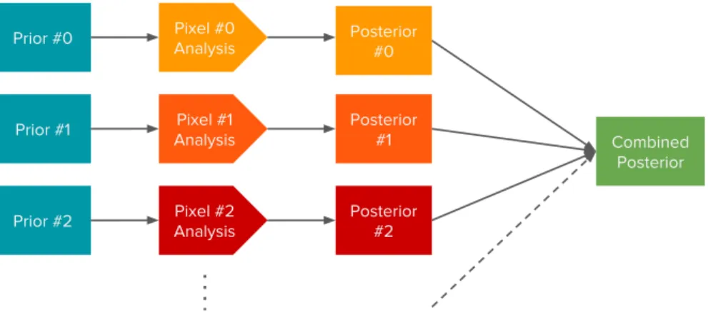
4.3.2 Posterior Product

We are also interested in a fast way to obtain parameter estimates for our model, e.g.

for quick comparisons of our data and model. Since we have 148 detectors with separate

models and data, we want to parallelize their analyses and combine them at the end.

(24)

The posterior we want to obtain is:

P _total (✓ | D) / P _total (D | ✓) · P (✓). (4.5) P _total (✓ | D) refers to eq. 4.1. In many cases we can express our prior in the following manner:

P (✓) =

n Y

_Pixel

i=1

P _i (✓). (4.6)

Combine eq. 4.1 with eq. 4.6 and we receive:

P _total (✓ | D) /

n Y

_Pixel

i=1

P _i (✓ | D _i ) ·

n Y

_Pixel

i=0

P _i (✓) /

n Y

Pixel

i=1

P _i (✓ | D _i ) · P _i (✓).

(4.7)

This implies that, under the circumstance that the likelihoods and priors are indepen- dent of other pixels, we can express the global posterior as the product of all individual posteriors. Again, a caveat is that we have to bin our posterior samples. Additionally, the priors are limited to individual pixel basis. However, this method is highly parallelizable, especially when using a computing cluster. In this work we used the facilities of the Na- tional Energy Research Scientific Computing Center (NERSC). Each pixel analysis can be handled independently; afterwards the posteriors can be combined. One can see this as a ’Bayesian Single-Pixel Fit’. Fig. 4.2 shows the procedure of this approach.

Martin Ha Minh, Fitrium Team BAT for First Tritium 18th July 2018 33

Posterior

#0

Posterior Pixel #1 #1

Analysis

Prior #0 Pixel #0

Analysis

Posterior Pixel #2 #2

Analysis

Posterior Product

Prior #1

Prior #2

Combined Posterior

Figure 4.2: Schematic diagram of the posterior product method. Each pixel is analyzed

separately in parallel; the binned posterior distributions are combined in end.

(25)

Chapter 5

The Gaseous ^83m Kr Source in the KATRIN Experiment

In summer 2017, in the phase leading up to the tritium measurements, we introduced a gaseous ^83m Kr source in the KATRIN experiment. The gaseous krypton source allows us to test the complete KATRIN setup as it will be used for the tritium phase. ^83m Kr emits monoenergetic conversion electrons at multiple energies, making it optimal for calibration purposes. This body of work focuses on the L 3 -32 line. The goal of the analysis is to show the how the BAT in combination with our models can be used to analyze the integral spectra, examine impact from systematic uncertainties, explore how di↵erent parameters correlate with each other, inquire information about our experimental setup, and test pixel combination methods.

5.1 Decay and Line Model

In the following we show the theoretical decay and spectral lines of ^83m Kr and describe our modelling thereof.

5.1.1 Decay

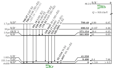
83m Kr has a half-life of 1.8 hours and is produced in the decay of ^83m Rb [McC15][V´en+18].

Fig. 5.1 shows the dcay scheme for this process.

It decays from its isomeric state while assuming an intermediate state in the process,

with energy level di↵erences of 32.2 keV and 9.4 keV respectively. This energy can be

emitted in the form of conversion electrons, which are quasi-monoenergetic. They are

therefore highly useful for the calibration of experiments detecting electrons, such as the

KATRIN experiment. While there are di↵erent lines in the ^83m Kr decay that can be

used for di↵erent purposes, we will focus on the L ₃ -32 line, corresponding to an expected

line position E _pos = 30472.2 eV and width = 1.19 eV. Reason for this is the high

(26)

42 3 Energy scale in KATRIN

9/2⁺ 0

stable <5.0 >8.5

7/2⁺ 9.406

155.1 ns 6.4 7.86

1/2⁻ 41.558

1.83 h

5/2⁻ 561.959

6 ps 61 6.05

(3/2⁻) 571.154

1.0 ps 29.4 6.35

5/2⁻ 690.53

10 ps 0.137 8.30

5/2⁺ 799.49

1.7 ps 0.90 6.87

5/2⁻ 0

86.2 d

83 37 Rb

Q= 919.4 keV

83 36 Kr

799.3 70.237

E2

790.1 50.66

(M1+E2)

⇡237.1 9<0.000

492

681.1 80.031

[E1]

648.9 70.085

E2

128.5 50.0016

[M1,E2]

119.3 20.018

(M1+E2)

529.5 94529.4(M1+E2) 562.1

70.0085 552.5

51216.0(E1) 520.3

99145 E2

32.151670 E3

9.4 057101

M1+E2

Figure 3.4: The decay scheme of

⁸³

Rb and

^83m

Kr as the second excited state of

⁸³

Kr. For the nuclear levels the following is indicated: half-life, spin-parity, energy in keV, branching ratio in % and log f t values. The nuclear transitions between the levels are indicated with energy in keV, intensity per

⁸³

Rb decay in % and multipolarity. The figure is based on ref. [McC15].

for the free atom B

_i^vac

, which refers to the vacuum level, plus small corrections that take into account recoil energies. This can be written as

E

i

= E + E

,rec

E

e,rec

B

_i^vac

, (3.41) where E

,rec

is the recoil energy after gamma emission and E

e,rec

is the recoil energy after electron emission. The term E + E

,rec

is the energy of the nuclear transition.

The K-shell (in spectroscopic notation 1 s

1/2

orbital) conversion electrons of the 32 keV transition, denoted as the K-32 electrons, have the binding energy of B

K

= 14.4 keV and thus the energy of E

K

= 17.8 keV which is desired in the tritium neutrino mass -decay experiments. Other conversion electrons such as L

3

-32 (2 p

3/2

) and L

1

-9.4 (2 s

1/2

) have energies of 30.5 keV and 7.5 keV, respectively, which are more remote from the tritium endpoint but which are also measureable by the MAC-E filter. An overview of the full

83m

Kr conversion electron spectrum, which is discrete in contrast to the continuous - spectrum, is shown in Fig. 3.5.

Due to finite lifetime of the vacancy, which is created after conversion electron emission, the electron energy distribution is not strictly sharp but has a certain spread which is comparable to the resolution of the MAC-E filter

⁴

. The energy distribution I (E) is

4

Also the lifetime of the nuclear excited state contributes to the spread of the electron energy distri- bution. However, in the case of

^83m

Kr this contribution is negligible.

Figure 5.1: Decay scheme of ^83m Rb into ^83m Kr. This figure is from [Sle15], based on [McC15].

intensity per decay of 37.8% as well as its line width similar in magnitude to the KATRIN spectrometer energy resolution.

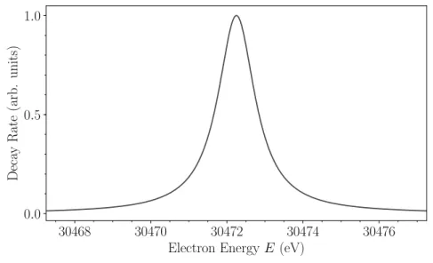
5.1.2 Di↵erential Spectrum

We use a Lorentzian function to describe the di↵erential shape of the line:

L(E, A, E _pos , ) = A

⇡

/2

(E E pos ) ² + ² /4 . (5.1)

E pos and describe the line position and line width (full width at half maximum) respec- tively; A describes the normalization factor. Fig. 5.2 plots an example spectrum.

5.1.3 Thermal Doppler E↵ect

Due to the non-zero temperature of the gas source, the shape is broadened by a thermal Doppler e↵ect. This is accounted for by convolving the Lorentzian function with a Gaus- sian function. This Gaussian is centered around zero and has a width = p

2EkT m/M ,

where T is the gas temperature, k is the Boltzmann constant, m is the electron mass,

and M is the mass of ^83m Kr. In this case the temperature T is set to 100 K to prevent

freeze-out on the beam tube walls. The mean of the Gaussian describes the flow of the

gas, which we here assume to be negligible. The resulting function is also known as the

Voigt function V .

(27)

30468 30470 30472 30474 30476 Electron Energy E (eV)

0.0 0.5 1.0

Deca y Rate (arb. units)

Figure 5.2: Lorentzian function describing the di↵erential decay rate of the monoenergetic

83m Kr L ₃ -32 line.

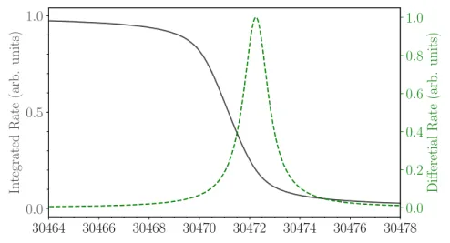
5.1.4 Integrated Spectrum

During the krypton measurements the gas density was low enough so that energy loss by electron scattering was negligible. This reduces the response function to the transmission function, Equation (2.5). The integrated spectrum I can then be described by:

I(qU, A, E _pos , ) = Z ₁

1 V (E, A, E _pos , )T(E, qU ) dE. (5.2) Fig. 5.3 shows an example for the integral and di↵erential spectrum. As the MAC- E filter works as an integrating filter, electrons from energetically higher lines can pass through the spectrometer to the FPD. For our analysis, we expect their rate constant in our small analysis window. We therefore add a constant term C to account for this o↵set.

The model is then as follows:

M(qU, E pos , , A, C) = I (qU, E, , A) + C. (5.3) Our parameters of interest in this case are the line position E _pos and the line width , while the normalization A and the constant o↵set C are nuisance parameters. The software used for this analysis is a combination of the Fitness Studio, a software framework for fitting models to data by Martin Slez´ ak [SK18], and the BAT.

5.1.5 Likelihood Function

The likelihood function we use is then:

(28)

30464 30466 30468 30470 30472 30474 30476 30478 0.0

0.5 1.0

In tegrated Rate (arb. units)

0.0 0.2 0.4 0.6 0.8 1.0

Di ff eretial Rate (arb. units)

Figure 5.3: Integrated rate of the ^83m Kr L ₃ -32 line superimposed with the corresponding di↵erential rate.

P (D, E _pos , , A, C) = Y

i

P h

D(qU _i ); M(qU _i , E _pos , , A, C) i

, (5.4)

where D(qU _i ) is the number of counts measured at the retarding potential qU _i and P (k; ) is the Poisson probability for measured counts k given expected counts .

5.2 Analysis of the L 3 -32 Line

With the analysis of the L ₃ -32 line of ^83m Kr we want to show the usability of BAT. First, we present statistical only analysis, then we discuss the systematic uncertainties during the measurement and how they are handled. Additionally, we test the pixel combination techniques. We also show an estimation of the relative energy resolution of the KATRIN experiment. Table A.1 shows the settings used in this analysis.

5.2.1 Choice of Priors

We choose non-informative priors for this analysis. For both our physical parameters the line position E _pos and the line width , as well as our nuisance parameters the amplitude A and the constant o↵set C, we use flat priors and restrict them to be positive.

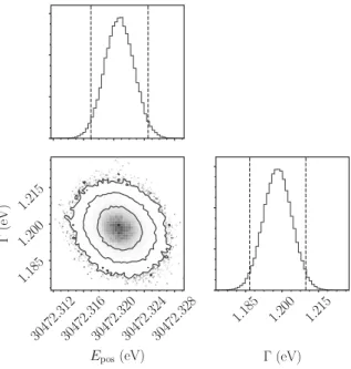
5.2.2 Uniform-Fits

We start by examining the uniform fit. Fig. 5.4 shows the posterior distributions for

E _pos and . For the mean of the posterior we obtain 95% credible intervals for E _pos =

(29)

30472 . 312

30472 . 316

30472 . 320

30472 . 324

30472 . 328

E

pos

(eV) 1 . 185

1 . 200 1 . 215

(eV)

1 . 185 1 . 200 1 . 215

(eV)

Figure 5.4: Marginalized posterior distributions for E _pos and from a uniform fit. The contours show the 68%, 95% and 99.7% credible intervals. The dotted lines indicate the 95% credible intervals.

[30472.317, 30472.325] eV and = [1.187, 1.210] eV. Fig. 5.5 shows the recorded spectrum as well as a model prediction using the obtained results.

5.2.3 Single-Pixel Fits

Next, we perform a single-pixel fit. Fig. 5.6 shows the marginalized posterior distributions and fig. 5.7 plots a fit for the innermost pixel. To inspect for pixel-dependent patterns, we plot the distribution of fit values across the FPD in fig. 5.8.

A dipole structure is visible in the heat map of the line position E _pos ; i.e. the inferred

line position of the pixels on the right side seem to be shifted towards higher values

compared to left side. There does not seem to be a pattern in the line width , or at

least it is not as extreme. At the moment we attribute this e↵ect to a misalignment of

the FPD [Cho18]. We will further investigate this in future measurements. In any case,

we can conclude that we should not continue using the uniform fits here, as it introduces

a systematic error by smearing the spectra. Since the number of events for the krypton

measurements is rather high, we will for now analyze the innermost pixel for the sake of

simplicity.

(30)

4000 6000 8000

Coun t rate (cps)

30466 30468 30470 30472 30474 30476 30478 30480 qU (eV)

2.5 0.0 2.5

Norm. residuals

Figure 5.5: Spectrum of the measured count rate and model predictions from the posterior

distribution for a uniform fit. The blue lines represent model predictions drawn from the

posterior distribution: We take 2000 MCMC samples, corresponding to multi-dimensional

parameter vectors, with which we calculate a model prediction for the spectrum; these

predictions can then be visualized as shown above. We use this method in all subsequent

spectral plots. The red items represent information from the posterior mean.

(31)

30472 . 50

30472 . 55

30472 . 60

30472 . 65

E

pos

(eV) 0 . 90

1 . 05 1 . 20 1 . 35

(eV)

0 . 90 1 . 05 1 . 20 1 . 35

(eV)

Figure 5.6: Marginalized posterior distributions for E _pos and from a fit for the innermost pixel. The contours show the 68%, 95% and 99.7% credible intervals. The dotted lines indicate the 95% credible region.

30 40 50 60 70

Coun t rate (cps)

30466 30468 30470 30472 30474 30476 30478 30480 qU (eV)

2.5 0.0 2.5

Norm. residuals

Figure 5.7: Spectrum of the measured count rate and model predictions from the posterior

distribution fit using the innermost pixel. The blue lines represent model predictions drawn

from the posterior distribution. The red items represent information from the posterior

mean.

(32)

Figure 5.8: Heat maps of the line position E _pos (left) and line width (right) relative to their respective means for a single-pixel fit. The excluded pixels are not filled. A dipole structure is visible in the heat map of E _pos .

5.2.4 Multi-Pixel Fits

We now want to test our pixel combination methods. We choose the first 40 pixels, corresponding to the 4 innermost pixels and the first 3 rings. For the chaining method, we start with a flat prior on E _pos and and use the marginalized posterior distribution for E _pos and of one analysis as the prior for the subsequent one. For the posterior product method we analyze each pixel separately and combine the results in the end by multiplying the marginalized posterior distributions. Fig. 5.9 shows a comparison of the marginalized posterior distributions for this analysis.

We can see that the marginalized posterior distributions generally agree in their shape and range up to a minuscule shift. However the posterior product has an uneven behaviour.

The posterior distributions of the individual pixels are shifted in position (see fig. A.2).

Therefore the common range is rather small. To accommodate for this, a finer binning is necessary. However, this increases the uncertainty on the bin content, due to the finite amount of samples, leading to an uneven behavior of the posterior shape. This propagates into the posterior product. A solution to this would be to have a longer run time for the MCMC to produce more samples.

Nevertheless we can produce credible intervals. The results are shown in table 5.1. We

can see that the credible intervals match very well, up to a small shift, as expected from

the visual inspection of the marginalized posteriors.

(33)

30472.57 30472.58 30472.59 30472.60 30472.61 30472.62 30472.63 Epos(eV)

0 25 50 75 100 125 150 175 200

P(Epos|D)

Posterior product Chaining

1.100 1.125 1.150 1.175 1.200 1.225 1.250 1.275 1.300 (eV)

0 5 10 15 20 25 30 35 40

P(|D)

Posterior product Chaining

Figure 5.9: Comparison of the the marginalized posterior distributions for E _pos (left) and (right) using di↵erent multi-pixel fit strategies. The number of samples in this analysis was not enough to accommodate for the fine binning necessary, leading to the uneven behaviour of the posterior product.

Table 5.1: 95% credible intervals for the line position E pos and the line width for di↵erent multi-pixel methods.

Method Line position E _pos Line width Chaining [30472.592, 30472.607] [1.156, 1.204]

Posterior product [30472.591, 30472.606] [1.152, 1.198]

(34)

5.3 Discussion of Systematic Uncertainties

The main source of systematic uncertainty we experience in the krypton measurements is the so-called high voltage ripple. Due to the 50 Hz frequency of the grid power’s alternating current, there is a small oscillating change of the retarding voltage applied to the main spectrometer. This e↵ect is exclusive to the krypton measurements analyzed in this thesis.

In the final measurement a post-regulation system will be applied. An electron that enters the main spectrometer experiences a retarding potential, and by extension a transmission function, that is slightly modified by the high voltage ripple. As the electrons are fast compared to the change of the high voltage we can postulate:

T ^⇤ (E, qU ) = 1

⇡ Z _⇡/2

⇡/2

T (E, qU + qA _HV · sin ) d , (5.5) where A _HV is the amplitude of the high voltage ripple, or the magnitude of the maxi- mum change of voltage from the set retarding potential qU . Pragmatically, A HV leads to an additional width in the integrated spectrum. This makes it difficult to estimate the extent of A _HV by fitting the data: The observed width _obs is a combination of the decay width _Kr and the width caused by the inseparable high voltage ripple _HV . This means that the contribution to the line width by one e↵ect can be absorbed by the other when fitting. The spectometer resolution also contributes a width, however it is here fixed by the magnetic fields.

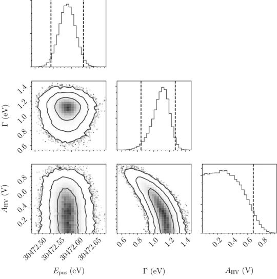
We can confirm this in practice: We set a positive definite flat prior on _HV and perform a fit for the innermost pixel. Figure 5.10 shows the posterior distributions for and A _HV . From its shape we cannot infer a value on A _HV , however we can set an upper limit of 673.7 mV at a 95% credible interval. The two-dimensional marginalized posterior distribution of and A _HV shows also an anti-correlation, as we expected.

Measurements estimate A _HV to 208 mV with a relative error of 20% [Are+18]. We will use this value to evaluate its impact on the measurements by setting a Gaussian prior with these values and performing a fit for the innermost pixel. Fig. 5.11 shows a knowl- edge update for the HV ripple amplitude A _HV and a comparison with the marginalized posterior distribution using a flat prior. From the knowledge update plot we can infer the contribution from the data gets dominated by the influence of the informative prior, as the shape of the marginalized posterior lines up almost exactly with the prior.

Fig. 5.12 shows a comparison of the marginalized posterior distributions for the line

position E _pos and the line width for di↵erent priors. We see the impact of the di↵erent

priors mostly with , as we expected: The higher the amplitude of the HV ripple, the

higher is its contributed width; A _HV and are strongly anti-correlated. The line width

can then decrease to compensate and keep the overall observed width constant. Therefore

we see a shift of the posterior in when we set A HV to non-zero values. Additionally the

posterior in widens if the HV ripple amplitude can also assume a large range of values.

(35)

0 . 6 0 . 8 1 . 0 1 . 2 1 . 4

(eV)

30472 . 50

30472 . 55

30472 . 60

30472 . 65

E

_pos

(eV) 0 . 2

0 . 4 0 . 6 0 . 8

A

HV

(V)

0 . 6 0 . 8 1 . 0 1 . 2 1 . 4

(eV)

0 . 2 0 . 4 0 . 6 0 . 8

A

_HV

(V)

Figure 5.10: Marginalized posterior distributions of the line position E _pos , line width ,

and HV ripple amplitude A _HV for a fit using the innermost pixel. From the experimental

data we obtain an upper limit of A HV < 673.7 mV at a 95% credible level.

(36)

0.0 0.2 0.4 0.6 0.8 A HV (V)

0 2 4 6 8 10

P ( A HV | D )

Prior Informative Flat

Figure 5.11: Knowledge update for the HV ripple amplitude with an informative prior using prior measurements and comparison with a marginalized posterior for a flat prior for the innermost pixel.

Since the line position E _pos is not strongly correlated to the observed line width, the e↵ect of di↵erent priors on the HV ripple amplitude A _HV is minuscule.

5.4 Estimating the Energy Resolution of the KATRIN Ex- periment

The total observed width is a combination of the natural line width of the L 3 -32 line, the contribution from the HV ripple, and the spectrometer resolution of the KATRIN experiment. With that knowledge, we can estimate the latter. We recall the relation for a MAC-E filter:

E

E = B _A B max

. (5.6)

The form showed here is the non-relativistic approximation. By fitting the ratio of

the magnetic fields we can make statements about the relative energy resolution. For

this analysis we use more informative priors; additionally to the prior on the HV ripple

amplitude A _HV we now also set a prior on the line width , as the resolution will correlate

strongly with any contribution to the observed width. The line width of the L ₃ -32 line

is not known very precisely, so we will set a conservative estimate of 20% relative error for

our Gaussian prior. The spectrometer resolution can vary freely under a flat prior.

(37)

30472.50 30472.55 30472.60 30472.65 30472.70 Epos(eV)

0.0 2.5 5.0 7.5 10.0 12.5 15.0 17.5

P(Epos|D)

Informative Flat AHVfixed

0.6 0.8 1.0 1.2 1.4

(eV) 0

1 2 3 4 5 6

P(|D)

Informative Flat AHVfixed

Figure 5.12: Comparison of marginalized posterior distributions of the line position E _pos (left) and line width (right) using di↵erent priors for a fit of the innermost pixel. The

”informative” prior is a Gaussian on the HV ripple amplitude with a 20% relative width centered around 208 mV, corresponding to the results of prior measurements. The poste- rior for the line width widens with a flat prior on A _HV due to the high correlation with A _HV . E _pos is not strongly correlated with A _HV and is thus barely a↵ected by di↵erent priors on A _HV .

Fig. 5.13 shows the marginalized posterior distributions for this analysis. As we ex- pected, the line width is strongly correlated with the energy resolution. The two- dimensional marginalized posterior for E/E and the HV ripple amplitude A _HV seems to not show a strong correlation; this is due to the constraint from the prior on A _HV . A rather unexpected correlation can be seen between E/E and the line position E pos . A widening of the energy resolution also leads to a widening of the transmission function, which will shift the center of the slope of the transmission function. This e↵ectively leads to higher observed energies.

The 95% credible intervals for the relative energy resolution is _E ^E = [3.27, 7.54] · 10 ⁵ ,

corresponding to [0.61, 1.40] eV at 18.6 keV. This is a highly satisfying result, as it covers

the expected value of 1.20 eV. From this we can deduce that the KATRIN experiment

fulfills the requirements for the MAC-E filter principle.

(38)

0 . 75 1 . 00 1 . 25 1 . 50

0 . 08 0 . 16 0 . 24 0 . 32

A

HV

30471 . 7

30472 . 0

30472 . 3

30472 . 6

30472 . 9

E

pos

(eV) 2

4 6 8

10

5

E /E

0 . 75 1 . 00 1 . 25 1 . 50 0 . 08 0 . 16 0 . 24 0 . 32 A

HV

2 4 6 8

10

⁵

E/E

Figure 5.13: Marginalized posterior distributions for the evaluation of the relative energy

resolution for a fit using the innermost pixel. The energy resolution strongly correlates

with the line width ; the correlation with the HV ripple amplitude A _HV is suppressed

by the constraint of its prior. The line position E pos is strongly correlated due to the

correlation of the energy resolution with the slope of the transmission function, leading to

a shift in the mean of detected energies. We obtain a 95% CI of E/E = [3.27, 7.54] · 10 ⁵ .

(39)

Chapter 6

First Tritium Data

In June 2018 we performed the First Tritium measurements. The purpose of this phase was to test the KATRIN experimental setup with tritium for the first time, to test the stability of the source parameters, and also to test our analysis tools with actual tritium data.

In this section we will first describe our modelling of the tritium spectrum. Then we will show our analysis strategies, examining both single- and multi-pixel fit analyses before we discuss the systematic uncertainties we identified and how we handle them.

6.1 Description of the Tritium Spectrum

The di↵erential decay rate of a tritium spectrum is derived from Fermi’s Golden Rule [OW08]:

d

dE = C · F (Z, E) p (E + m _e )E _⌫ X

i

| U _ei | ² q

E _⌫ ² m ² _i ⇥(E _⌫ m _i ). (6.1) With natural units so that c = 1 and ¯ h = 1. C = ^G _2⇡

²^F3

cos ² ✓ C | M | ² , where G F is the Fermi constant, ✓ _C is the Cabibbo angle, and M is the nuclear matrix element. The Fermi function F (Z, E) takes the Coulomb interaction between the emitted electron and the daughter nucleus with the charge Z into account. p, E, and m _e are the momentum, energy, and mass of the electron, respectively.

To account for the di↵erent neutrino flavors it is necessary to sum over the mass eigenstates m _i . The fraction of contribution of each term is determined by the absolute square of the neutrino mass mixing elements U _ei . Due to the resolution of KATRIN, we can simplify by considering the e↵ective electron neutrino mass m ² _⌫ = P

i | U ei | ² m ² _i

[FS03]. As the logarithm of the likelihood is parabolic in m ² _⌫ , not m _⌫ , we can say that our

observable is not the e↵ective electron neutrino mass but the e↵ective electron neutrino

mass squared.

(40)

E _⌫ describes the neutrino energy E _⌫ = E ₀ E, where E ₀ is the so-called endpoint energy of the tritium spectrum, the maximum energy an electron can assume with m ⌫ = 0.

The Heaviside function ⇥ ensures energy conservation.

Molecular tritium decays as follows:

T ₂ ! ³ HeT ⁺ + e + ¯ ⌫ _e . (6.2)

The resulting daughter molecule can then end up in an excited rotational, vibrational, or electronic state. To accommodate for this, the formula for the neutrino energy E ⌫ can be amended:

E _⌫ ! E ˜ _⌫ = E ₀ V _f E. (6.3)

V _f is the energy associated with the final state f. Equation (6.1) then has to be expanded with the summation over the final states f and their probabilities P _f to decay into:

D(m ² _⌫ , E ₀ , E ) = C · F (Z, E)p(E + m _e ) X

f

P _f E ˜ _⌫

q E ˜ _⌫ ² m ² _⌫ ⇥( ˜ E _⌫ m _⌫ ). (6.4)

The final state distributions, that indicate which final states f can be assumed with probability P _f and energy V _f , are known from theoretical calculations. Their inclusion and accuracy is of utmost importance for the precise measurement of the neutrino mass. In this work, we use the calculations from [Dos+06] [DT08]. Fig. 6.1 shows the distribution of the final states used in this analysis.

0 2 4

Final State Energy V f (eV) 0.00

0.02 0.04 0.06

Probabilit y

25 50 75 100

DT T 2

Figure 6.1: Binned final state distributions used in this work for di↵erent isotopologues.

The shift of the bins between the models are purely for visual enhancement.

(41)

Equation (6.4) is the form we use in this work to model the tritium spectrum. If we integrate it with the Response Function eq. (2.7) we obtain the Integrated Spectrum I:

I (qU, m ² _⌫ , E ₀ ) = Z E

0

qU

_min

R(qU, E ) · D(m ² _⌫ , E ₀ , E) dE. (6.5)

18100 18200 18300 18400 18500 18600

Retarding Potential qU (eV) 0

1 2 3 4

In tegral Rate I (arb. units)

10 ¹⁴

Figure 6.2: Example of the integrated spectrum with m ² _⌫ = 0 and E 0 = 18575 eV for KATRIN design values.

Fig. 6.2 plots an example for an integrated spectrum. Due to solid states e↵ect, the observed electron energy is shifted by the di↵erence of the work functions of the source and the spectrometer. This e↵ectively leads to a shift of from the true values E the observed energies qU :

E = qU ( _Source Spectrometer ). (6.6)

A constant shift of the observed energies will not influence our measurement of the neutrino mass [Sle15]. However it will influence values of the endpoint E ₀ . At the moment we do not have a precise handle on the magnitude of this shift. For now we assume a conservative estimate of ± 1 eV. We therefore denote our observed endpoint as the e↵ective endpoint E ₀ ^e↵ .

Additionally we expand the model by multiplying the Integrated Spectrum with a normalization constant A as well as adding a constant o↵set C as a background model:

M (qU, m ² _⌫ , E ₀ ^e↵ , A, C) = A · I(qU, m ² _⌫ , E ₀ ^e↵ ) + C. (6.7)

In the neutrino mass analysis the parameter of interest is obviously m ² _⌫ . However, in

our First Tritium measurement phase we do not attempt to measure the neutrino mass,

submitted in partial fulfillment of the requirements for the degree of

Max Planck Institute for Physics Fakult¨ at f¨ ur Physik Technische Universit¨ at M¨ unchen

A thesis