in fulfillment of the requirements for the degree “Dr. rer. Nat.”

Tropopause Inversion Layer: 

High­Resolution GPS­RO Observations  and Reanalyses

Dissertation

in fulfillment of the requirements for the degree “Dr. rer. Nat.”

of the Faculty of Mathematics and Natural Sciences at Christian­Albrechts­Universität zu Kiel

Submitted by:

Robin Pilch Kedzierski

Kiel, 2016

Date of the oral examination: 2016.10.17 Approved for publication: 2016.10.17

Signed:  Dr. Wolfgang J. Duschl, Dean

Abstract / Zusammenfassung 1

1 Introduction 3

1.1 What is the Tropopause Inversion Layer? . . . . 3

1.2 Observed Variability of the TIL . . . . 5

1.2.1 Tropics . . . . 5

1.2.2 Extratropics . . . . 7

1.3 Processes enhancing the TIL . . . . 9

1.4 Representation of the TIL in models and reanalyses . . . . 13

1.5 Goals of this Thesis . . . . 15

2 Methods 17 2.1 Datasets . . . . 17

2.1.1 GPS Radio-Occultation profiles . . . . 17

2.1.2 ERA-Interim reanalysis . . . . 20

2.2 TIL diagnostics . . . . 21

2.3 Wave signal extraction . . . . 22

2.3.1 Tropics . . . . 22

2.3.2 Extratropics . . . . 24

3 The Tropical Tropopause Inversion Layer: Variability and Modulation by Equa- torial Waves 27 4 The Extratropical Tropopause Inversion Layer 59 4.1 Synoptic-Scale Behavior . . . . 60

4.2 Modulation by Extratropical Waves . . . . 79

5 Tropopause Sharpening by Data Assimilation 111

6 Conclusions and Outlook 131

6.1 Conclusions . . . 131

Acknowledgements 145

List of figures 147

Abbreviations 149

Declaration 151

as a ’transition’ between the two layers and consequently has properties from both. Within this region, a fine-scale feature is located: the Tropopause Inversion Layer (TIL), which consists of a sharp temperature inversion at the tropopause and the corresponding high static stability values aloft. The latter theoretically affects the dispersion relations of atmospheric waves like Rossby or Inertia-Gravity waves and hampers stratosphere-troposphere exchange (STE), which is why the TIL is established as an important feature of the UTLS.

The present thesis aims to improve the observational knowledge about the TIL by an- alyzing high-resolution GPS radio-occultation (GPS-RO) data globally. The focus is on day-to-day and synoptic-scale TIL variability, a novel approach to build upon the climato- logical point of view from earlier TIL studies. Daily snapshots of the horizontal structures of TIL strength show the first evidence of a relationship between a stronger (weaker) TIL and near-tropopause divergent (convergent) flow in the tropics. In the extratropics, the TIL within mid-latitude ridges in winter is as strong or stronger than the TIL in polar summer, which is strongest in the seasonal zonal-mean according to previous studies.

Also, a dynamical mechanism for TIL enhancement is studied and quantified: the transient tropopause modulation by equatorial and extratropical waves, and the resulting net TIL enhancement. In the tropics, equatorial waves explain an important part of the observed TIL strength, with Kelvin, Rossby and inertia-gravity waves as main contributors. In the extratropics, the modulation by planetary and synoptic-scale waves explains the observed TIL strength at mid-latitudes almost entirely, while also being dominant in polar regions. The role of this transient wave modulation mechanism has not been investigated in TIL literature, and its quantification from GPS-RO observations puts it among the most important TIL enhancing processes.

Lastly, the paradigm that data assimilation worsens the representation of the TIL in reanalyses, valid a decade ago, has been tested in modern systems: the ERA-Interim reanaly- sis and the ECMWF forecasts. Both systems show TIL improvement by data assimilation increments, updating the earlier status quo.

As a whole, this thesis significantly improves our knowledge about observed properties

of the TIL and the mechanisms responsible for its formation and maintenance, and shows

that reanalyses are a valuable tool for TIL research.

Tropopause Inversion Layer (TIL), welche durch eine markante Temperaturinversion an der Tropopause und eine daraus resultierende hohe statische Stabilität oberhalb dieser charakterisiert ist. Letztere beeinflusst theoretischen Betrachtungen zufolge die Dispersionsrelationen atmosphärischer Wellen (z.B.

Rossby- oder Schwerewellen) und behindert den stratosphärisch-troposphärischen Austausch (STE), weshalb der Erforschung der TIL als Bestandteil der UTLS besondere Aufmerksamkeit gewidmet wird.

Ziel der vorliegenden Arbeit ist eine verbesserte Analyse der TIL und der mit ihr verbundenen Prozesse anhand von hochaufgelösten globalen Daten auf Basis der GPS Radio-Okkultation (GPS-RO).

Der Analyseschwerpunkt liegt in der Untersuchung der Variabilität auf täglichen und synoptischen Skalen. Im Gegensatz zu früheren Studien auf klimatologischer Basis kann diese Herangehensweise als neuer Ansatz verstanden werden, da tägliche Momentaufnahmen der horizontalen Strukturen der TIL es erlauben, erstmals einen Zusammenhang zwischen einer stark (schwach) ausgeprägten TIL und divergenten (konvergenten) Strömungen nahe der Tropopause in den Tropen aufzuzeigen. In den Extratropen ist die TIL im Winter im Bereich von atmosphärischen Rücken in den mittleren Breiten ebenso stark oder sogar stärker ausgeprägt als die TIL im polaren Sommer, die entsprechend früherer Studien im zonalen Mittel am stärksten ausgeprägt ist.

Desweiteren wird in dieser Arbeit ein dynamischer Prozess untersucht und quantifiziert, der zu einer Verstärkung der TIL führt: Die kurzlebige Tropopausenmodulation aufgrund von äquatorialen und extratropischen Wellen sowie die resultierende Gesamtverstärkung der TIL. Es wird gezeigt, dass die TIL in den Tropen im wesentlichen durch äquatoriale Wellen, hauptsächlich Kelvin-, Rossby- und Trägheitsschwerewellen, verstärkt wird, während in den mittleren wie auch polaren Breiten die Modulation durch Wellen auf planetarer sowie synoptischer Skala dominiert. Der Einfluss des in dieser Arbeit untersuchten Wellen-Modulations-Mechanismus auf die TIL wurde in früheren Studien zur TIL nicht diskutiert, obwohl seine Quantifizierung mit Hilfe der GPS-RO Beobachtungen in dieser Studie zeigt, das er als einer der wichtigsten Verstärkungsprozesse der TIL angesehen werden muss.

Schließlich wird das vor einem Jahrzehnt gültige Paradigma, dass die Datenassimilation die Repräsen- tation der TIL in Reanalysen verschlechtert, anhand neuer Datensätze (ERA-Interim und EZMW- Vorhersagen) überprüft. In beiden Datensätzen ist die TIL durch Fortschritte in der Datenassimilation deutlich realistischer dargestellt, was die früheren Feststellungen über die Qualität der Reanalysedaten revidiert.

Zusammengefasst, liefert diese Arbeit wichtige Beiträge, um unsere Kenntnisse über das Erschein- ungsbild der TIL sowie die für ihre Bildung und Aufrechterhaltung relevanten Prozesse zu erweitern.

Außerdem zeigt sie, dass die aktuellen Reanalysedaten ein wertvoller Tool für die Untersuchung der TIL

1 Introduction

1.1 What is the Tropopause Inversion Layer?

The Tropopause Inversion Layer (TIL) is a narrow region characterized by a sharp temperature inversion at the tropopause and the corresponding enhanced static stability located right above. The TIL is a fine-scale feature of about 1 km depth, discovered by tropopause-based averaging of high-resolution radiosonde measurements by Birner et al. [2002] and Birner [2006]. Satellite Global Positioning System radio occultation observations (GPS-RO) show that the TIL is present globally [Grise et al., 2010].

Figure 1.1 shows vertical profiles of temperature and static stability (N

) at mid-latitudes, comparing the tropopause-based and ground-based averaging techniques (from Birner [2006]).

Fig. 1.1 Climatological profiles of temperature (left) and buoyancy frequency squared (right) at

∼ 45°N from high-resolution radiosondes (1998-2002). Dotted lines are a ground-based average, solid lines are a tropopause-based average, and the dashed lines denote the US standard atmosphere profiles.

Figure from Birner [2006].

Only when averaging is performed with respect to the tropopause level as the reference,

the temperature inversion and maximum in N

are clearly visible in Fig. 1.1 (solid black

lines), with very sharp gradients across just a few hundred meters: therefore observations

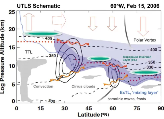
the troposphere and the stratosphere as a consequence of the transition between these two layers. In the tropics this transition layer is known as the Tropical Tropopause Layer (TTL, Fueglistaler et al. [2009]), and at other latitudes as the extratropical upper-troposphere and lower-stratosphere (Ex-UTLS, Gettelman et al. [2011]). The TIL is established as an important feature of the UTLS [Gettelman et al., 2011] since it shows that the transition between the troposphere and the stratosphere is rather sharp at a certain and narrow altitude range. Figure 1.2 shows a UTLS schematic with the location of the TIL and the tropopause structures and processes that take place at different latitudes (from Gettelman et al. [2011]).

Fig. 1.2 Schematic snapshot of the extratropical UTLS, as a meridional section in the Northern Hemisphere. Shown are zonal winds (solid black lines), potential temperature surfaces (dashed black lines), the thermal tropopause (red dots) and the dynamical tropopause (2 PVU surface, light blue solid line). Illustrated are sketches of the TIL (green shading), the Brewer-Dobson Circulation (red arrows at the top), quasi-isentropic exchange (wavy red arrows), cross-isentropic exchange (wavy orange arrows) and clouds and fronts (gray shading). The extratropical UTLS is represented by blue shading, including the ’mixing layer’ (dark blue shading). Figure from Gettelman et al. [2011].

What are the implications of the TIL? As shown in Fig. 1.1, the positive gradient of

temperature right above the tropopause translates into high N

values, distinctly above those

found throughout the stratosphere. High static stability suppresses vertical motion, therefore

et al., 2009; Kunz et al., 2009; Schmidt et al., 2010]. Hence the TIL could significantly influence the stratosphere-troposphere exchange (STE) and the composition of both layers.

Also, N

is a parameter used in different atmospheric wave theory approximations [Andrews et al., 1987], so the TIL shall theoretically affect the dispersion relations of Rossby and Inertia-Gravity waves.

To summarize, the TIL is a relatively recent and growing topic of research, whose study needs observations with high vertical resolution due to its fine-scale nature. The TIL could potentially play an important role in the chemical composition and the dynamics of the troposphere and the stratosphere, as well as the interactions between these two atmospheric layers.

1.2 Observed Variability of the TIL

This subsection will introduce the properties of the TIL which have been observed thus far. A subdivision between the tropics and extratropics applies given the difference in the dominant physical processes between these regions: radiative-convective balance in the tropics and baroclinic wave dynamics in the extratropics [Held, 1982]; therefore the TIL shows a different behavior in each region. The proposed mechanisms that drive the observed TIL variability will be discussed in the next subsection 1.3.

1.2.1 Tropics

Research about the TIL has focused very little in the tropics. The global TIL study by Grise et al. [2010] includes the horizontal and vertical variability of the tropical TIL, making it the most detailed description of TIL properties in the tropics. Bell and Geller [2008] showed the TIL from one tropical radiosonde station, and Wang et al. [2013] reported a slight weakening of the tropical TIL between 2001-2011. In the study by Grise et al. [2010] it was found that the strongest tropical TIL (as the mean N

in the layer 0-1 km above the tropopause) is centered at the equator, peaking during NH winter. Later studies by Son et al. [2011] and Kim and Son [2012] agree well with this seasonality and location of the tropical tropopause sharpness.

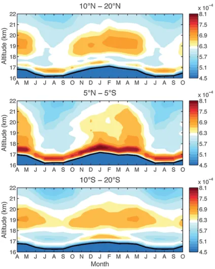
Figure 1.3 shows the seasonal cycle of the vertical tropopause-based N

structure in

the subtropics and the equator (from Grise et al. [2010]). The tropopause is higher in

winter throughout the tropics, which is related to the seasonal cycle of the stratospheric

Fig. 1.3 Seasonal cycle of the monthly tropopause-based N

vertical profile (color shading) at the NH subtropics, the equator and the SH subtropics. The black solid line represents the tropopause. Figure from Grise et al. [2010].

In the layer right above the tropopause, the equator shows the highest N

values, peaking in winter. In the subtropics, both hemispheres show a stronger TIL during their respective summer months, while another deeper region of enhanced N

, centered at 19 km height, forms during NH winter. This second subtropical maximum in N

at 19 km is related to the large seasonal cycle of temperature and ozone within that altitude range [Randel et al., 2007b]. The fact that the highest N

values right above the tropopause are centered around the equator indicates that the tropical TIL is strongly influenced by equatorially-trapped wave modes.

Indeed, the seasonal-mean horizontal structure of the TIL in the tropics is reminiscent

of the equatorial stationary wave response associated with climatological deep convection

quasi-biennial oscillation (QBO, Baldwin et al. [2001]).

1.2.2 Extratropics

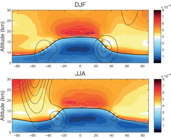
Studies about observational properties of the extratropical TIL are more numerous. Seasonal climatologies of the zonal-mean TIL show that it is strongest during polar summer, while another relative maximum in TIL strength is observed in mid-latitude winter [Birner, 2006;

Grise et al., 2010; Randel and Wu, 2010; Randel et al., 2007a]. This is shown in the latitude- height N

seasonal tropopause-based climatologies in Figure 1.4 (from Grise et al. [2010]).

Note that both maxima in extratropical TIL strength during polar summer and mid-latitude winter are still below the high N

values observed right above the tropical tropopause and centered at the equator.

Fig. 1.4 Seasonal zonal and tropopause-based mean N

global vertical structure (color shading), for

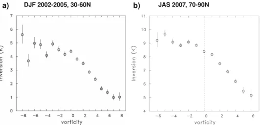
extratropical TIL strength. Observations show a stronger (weaker) TIL within anticyclones (cyclones) at all extratropical latitudes and seasons. Figure 1.5 shows this relationship in mid-latitude winter (left, from Randel et al. [2007a]) and polar summer (right, from Randel and Wu [2010]) as the dependence of stronger (weaker) TIL with collocated anticyclonic (cyclonic) relative vorticity. This relationship comes together with higher (lower) tropopauses within anticyclones (cyclones).

a) DJF 2002­2005, 30­60N b) JAS 2007, 70­90N

Fig. 1.5 Diagrams of relative vorticity (10

s

) versus TIL strength, as the temperature difference in K between the tropopause and 2 km above. (a) Mid-latitude winter; (b) polar summer. Figures from Randel et al. [2007a] and Randel and Wu [2010].

Polar vortex dynamics also influence the TIL: [Grise et al., 2010] found stronger high- latitude TIL correlated with downward-propagating positive N

and easterly wind anomalies that result from strong vortex disturbances, which is supported by a case study of major sudden stratospheric warmings (SSW) by Wargan and Coy [2016]. On the other hand, the Southern Hemisphere polar winter TIL is nearly absent [Tomikawa et al., 2009], since the polar vortex is strong, stable and cold there.

And finally, inertia-gravity waves (IGW) can affect the TIL and viceversa: a study with

one US radiosonde station [Zhang et al., 2015] showed that the upward propagation of

IGW is inhibited by the TIL, and also that the TIL can cause IGW breaking from shear

instability, which subsequently strengthens the TIL (see section 1.3 for more details about

the mechanism).

1.3 Processes enhancing the TIL

The present consensus about what forces the TIL is that a blend of different mechanisms, whose dominance varies with season and latitude, are responsible for its formation and maintenance. As shown in Fig. 1.1 in section 1.1, the TIL consists of a sharp temperature inversion at the tropopause, and the resulting temperature gradient right above the tropopause causes its high N

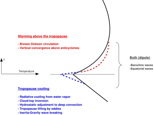
values. Therefore, processes making this temperature gradient larger will effectively enhance the TIL. This can be accomplished in two ways: by cooling the tropopause and/or warming aloft, as sketched in Figure 1.6. The processes that have been proposed to enhance the TIL will be disclosed in the following paragraphs.

Tropopause cooling

­ Radiative cooling from water vapor

­ Cloud­top inversion 

­ Hydrostatic adjustment to deep convection

­ Tropopause lifting by eddies

­ Inertia­Gravity wave breaking Warming above the tropopause

­ Brewer­Dobson circulation

­ Vertical convergence above anticyclones

Both (dipole)     ­Baroclinic waves     ­Equatorial waves Temperature

z

Fig. 1.6 Sketch of TIL enhancement by different processes: tropopause cooling (blue dashed line) and warming aloft (red dashed line) on a generic tropopause-based temperature profile (solid black line) similar to that in Fig. 1.1.

Tropopause cooling

- Radiative cooling from water vapor: the strong gradient of water vapor across the

tropopause leads to a differential cooling around the tropopause. This was first proposed by

Randel et al. [2007a] and later supported by Hegglin et al. [2009]; Kunz et al. [2009]; Randel

and Wu [2010]. A high-resolution model study by Miyazaki et al. [2010a,b] showed that this

temperature inversion generally found at the top of convective [Biondi et al., 2012] and non-convective cirrus clouds [Taylor et al., 2011]. Note that cirrus cloud occurrence near the tropopause is more frequent. Although near-tropopause clouds and the TIL have not been linked in scientific literature thus far, we suggest that a cloud top near the tropopause would have a TIL enhancing effect.

- Hydrostatic adjustment to deep convection: this is a purely dynamical response to compensate the pressure gradients from tropospheric warming, that extend above the heating.

Ascent and adiabatic cooling act to diminish these pressure gradients with height, cooling the tropopause region above the deep convective tower. Holloway and Neelin [2007] described the hydrostatic adjustment mechanism, and Paulik and Birner [2012] showed that the negative temperature signal near the tropical tropopause can be found a few thousand kilometers away from the convective region. This mechanism could be important for TIL enhancement in the tropics, which has not been studied yet.

- Tropopause lifting by eddies: model experiments have shown that dry dynamics explain an important part of the extratropical TIL behavior. Baroclinic waves have embedded cy- clones and anticyclones, and balanced dry dynamics produce a higher and colder tropopause within anticyclonic flow in idealized model experiments [Wirth, 2003, 2004]. This is con- sistent with the findings by Randel and Wu [2010]; Randel et al. [2007a], who observed higher tropopauses within anticyclonic flow together with stronger TIL. As shown in Figure 1.5 (section 1.2), the TIL relationship with relative vorticity is present at all extratropical latitudes.

- Inertia-Gravity wave breaking: a baroclinic life cycle experiment by Kunkel et al. [2014]

showed transient TIL modulation by the presence of IGWs and proposed a mechanism of persistent TIL enhancement from IGW breaking. The study by [Zhang et al., 2015] with one US radiosonde station supports this hypothesis by finding that the strong wind shear above the tropopause causes instability and breaking of IGWs, inducing wave energy dissipation, turbulence and downward heat flux, which in turn leads to a net cooling of the tropopause.

Warming above the tropopause

- Brewer-Dobson circulation: in a model experiment Birner [2010] proposed that the

downwelling branch of the Brewer-Dobson circulation should produce dynamical heating

above the tropopause. This is supported by a case study of major SSWs by Wargan and

Coy [2016], who showed a high-latitude TIL enhancement by SSWs, when their downward-

2016], which is accelerated during these events in agreement with Andrews et al. [1987].

- Vertical convergence above anticyclones: model experiments showed an onset of a secondary circulation between the cyclone and anticyclone embedded within a baroclinic wave Wirth [2004]; Wirth and Szabo [2007] which induces a heating above the tropopause in anticyclones. Vertical divergence above cyclones reduces the TIL strength, but only partly counteracts the TIL enhancement over anticyclones, which dominate the zonal mean.

Dipole by waves

- Baroclinic waves: as explained in the previous paragraphs, baroclinic waves effectively form a dipole of tropopause cooling and warming aloft through separated mechanisms acting at the same time: tropopause lifting and vertical convergence above anticyclonic flow [Wirth, 2003, 2004; Wirth and Szabo, 2007], which are explained by balanced dry dynamics. An idealized model experiment with only dry, synoptic-scale dynamics by Son and Polvani [2007] was able to partly explain the seasonality and latitude-dependence of the extratropical TIL strength which follows the amount of baroclinic wave activity. Also, baroclinic wave breaking skews the relative vorticity distribution near the tropopause towards anticyclonic values [Erler and Wirth, 2011], further increasing the dominance of anticyclonic TIL in the zonal-mean.

- Equatorial waves: since the tropical TIL strength is centered at the equator, the role of equatorially-trapped wave modes has to be important for the formation of the TIL in the tropics [Grise et al., 2010]. An important part of the equatorial wave spectrum is coupled to convection [Wheeler and Kiladis, 1999], so the aforementioned tropopause cooling from hydrostatic adjustment to deep convection [Holloway and Neelin, 2007; Paulik and Birner, 2012] can be included in this dipole, although convection can be independent of equatorial waves as well, and equatorial waves can also propagate freely. Kim and Son [2012] reported that the dominant modes of temperature variability at the tropopause region were Kelvin waves and the Madden-Julian oscillation (MJO, Madden and Julian [1994]). Equatorial wave temperature anomalies show lower-stratospheric warming and tropopause cooling in composites [Kim and Son, 2012] and average signatures on the long-term mean profile [Grise and Thompson, 2013], but their effect on the strength of the TIL has not been studied.

It has to be noted that all the mechanisms disclosed above target permanent and ir-

reversible effects on TIL strength. Little attention has been payed to the contribution of

atmospheric waves just by being present in the tropopause region, i.e. by a transient and

reversible modulation of the temperature structures near the tropopause. Extratropical waves

shown schematically in Figure 1.7.

z

Transient tropopause  modulation by waves

+ +

­ ­

­ ­

Longitude

Fig. 1.7 Schematic of transient tropopause modulation by an idealized wave with westward vertical tilt, as a snapshot of the wave’s temperature anomalies (dashed contours: positive red, negative blue) and the undulating tropopause (thick solid grey line). Figure from Pilch Kedzierski et al. [2016b].

Tropopause height, usually the coldest point at the uppermost troposphere, would vary zonally as a consequence of the wave anomaly structure. The zonal-mean tropopause height, the zonal-mean (ground-based) temperature or N

structure are not affected by the instantaneous tilted wave structure as in Fig. 1.7. However, the tropopause-based mean of the wave anomaly would turn to be a dipole of tropopause cooling and warming above, resulting in N

increase right above the tropopause, yielding a TIL. Once the wave is away from the tropopause or dissipated, it would not modulate the tropopause any more, but could still affect the TIL in other ways.

It would be of interest to know how much of the TIL is the result of the mere presence

of transient atmospheric waves, which enables to separate the instantaneous modulation of

the tropopause (and net TIL enhancement in the tropopause-based mean as in Fig. 1.7) from

other permanent TIL forcings as disclosed before in this section. The mechanism showed in

Fig. 1.7 has not been studied or quantified in any literature so far, thus being of great value

for increasing the knowledge about the processes that enhance the TIL: see section 1.5 for

more details about the goals of this thesis.

1.4 Representation of the TIL in models and reanalyses

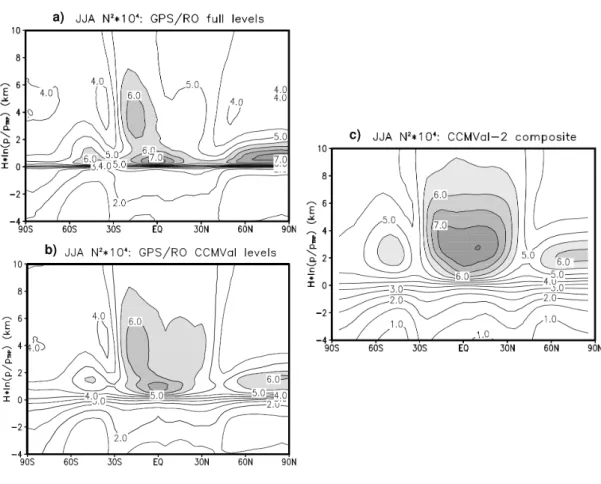
The TIL is a fine-scale feature whose properties can only be captured by data of high vertical resolution ( ∼ 100 m), i.e. GPS radio occultation (GPS-RO) profiles by satellites, and high- resolution radiosonde measurements. Atmospheric models are very limited in this sense, generally having a vertical resolution near the tropopause of around 1 km. Hegglin et al.

[2010] and Gettelman et al. [2010] compared the TIL in various models within the Chemistry Climate Model Validation project 2 (CCMVal-2). They also degraded the vertical resolution of GPS-RO observations to the models’ standard pressure levels in order to eliminate vertical resolution as a source of differences.

a)

b)

c)

Fig. 1.8 Comparison of the representation of the TIL in (a) full resolution GPS-RO observations, (b) GPS-RO degraded to model resolution, and (c) CCMVal-2 models. Figure from Gettelman et al.

[2010].

Figure 1.8 shows a latitude-height NH summer climatology of tropopause-based N

from

Gettelman et al. [2010].

It can be observed that especially in the extratropics the modeled TIL (Fig. 1.8 c) is too weak, too deep and very far away from the tropopause compared to the observed TIL from GPS-RO data at full vertical resolution (Fig. 1.8 a). When the vertical resolution of GPS-RO is degraded, the N

values above the tropopause (Fig. 1.8 b) are similar to those from the CCMVal-2 models, but still much closer to the tropopause, suggesting that the coarser vertical resolution in the models is not the only issue that causes a rather poor representation of the TIL. Despite this bias in the CCMVal-2 models, with weaker TIL and further away from the tropopause, its seasonality and latitude-dependence are well captured [Gettelman et al., 2010; Hegglin et al., 2010].

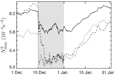
Birner et al. [2006] investigated the TIL in two data assimilation systems, the NCEP/NCAR reanalysis [Kalnay et al., 1996], and the Canadian Middle Atmosphere Model assimilating observations (CMAM+DA, Polavarapu et al. [2005]); both with similar vertical resolution of roughly 1km near the tropopause and the same three-dimensional variational (3D-Var) data assimilation technique. Birner et al. [2006] found that the TIL from the free-running CMAM was stronger than the TIL from CMAM with data assimilation and the NCAR reanalysis, therefore suggesting that data assimilation smooths out the sharp gradients that lead to the formation of the TIL. This is well illustrated in Fig. 1.9, that shows the response of the TIL strength to data being assimilated into the CMAM model.

Fig. 1.9 Time series of TIL strength as N

, from December 2001 to the end of January 2002. Line

types denote different latitudes: global mean (solid), NH mid-latitudes (45°N-75°N, dotted), SH

drops dramatically in Fig. 1.9 and remains low while data is assimilated (grey shading). As soon as data assimilation is switched off (1 Jan), the TIL starts recovering slowly. Therefore it is accepted that the TIL in a model gets worse once data is assimilated, as it is the case in reanalyses.

It has to be pointed out that GPS-RO data could not be assimilated at the time of the study by Birner et al. [2006], and that the models as well as the assimilation techniques have improved and are more sophisticated nowadays. Recently, modern reanalyses have been used to study the TIL, as is the case in Gettelman and Wang [2015] who produced a set of TIL diagnostics from ERA-Interim [Dee et al., 2011], and Wargan and Coy [2016]

who investigated the TIL in a case study of a major SSW in the Modern-Era Retrospective Analysis for Research and Applications version 2 (MERRA-2, Bosilovich and Coauthors [2015]; Molod et al. [2015]), proving both reanalyses useful for studying the TIL. Therefore the question arises whether data assimilation still makes the TIL worse in modern reanalyses.

1.5 Goals of this Thesis

This thesis broadly aims to increase the knowledge about TIL properties, the processes that lead to its formation/maintenance/enhancement and how data assimilation affects TIL representation in models. The goals of this thesis can be summarized into three main points, each of which groups several scientific questions, as disclosed below:

(a) Discover more TIL properties from observations: current knowledge about TIL properties is from climatologies, and smaller space and time-scales have not been explored yet.

- How does the real-time TIL look like? Most of the observed properties of the TIL, like the seasonality and latitude-dependence of its strength, were derived from climatologies, i.e. long-term means [Birner, 2006; Grise et al., 2010]. At synoptic-scales, its relationship with cyclonic-anticyclonic flow is known as seasonal averages binned by collocated relative vorticity [Randel and Wu, 2010; Randel et al., 2007a]. Snapshots of the horizontal structures of the TIL from observations will give a novel approach to study its day-to-day, synoptic-scale behavior.

- Done the above, can we make new links between the observed TIL and near-tropopause

meteorological processes? The synoptic-scale behavior of the TIL can be linked to ongoing

literature from model experiments (see section 1.3) but still await observational evidence.

(b) Quantify the transient TIL modulation by atmospheric waves: this mechanism for TIL enhancement has not been investigated in literature and could play an important role.

- How much of the TIL comes from the instantaneous tropopause modulation by waves?

Wave temperature anomalies and tropopause structures as sketched in Fig. 1.7 can be obtained from gridded GPS-RO observations (see section 2, Methods). Separating the relative contribution for TIL enhancement that is transient from other permanent processes can help to put their roles into context, which would be of high interest for the scientific community.

- What other processes enhance the remaining TIL without the wave signal? The vertical structure and time variability of the remaining N

structures without the wave signal can give very useful hints about what processes cause it, a valuable secondary result of the quantification of the TIL wave modulation.

(c) Test the hypothesis of Birner et al. [2006] in modern reanalyses: the study by Birner et al. [2006] is, up to date, the only one investigating the effect of data assimilation on the modeled TIL. A decade ago, data assimilation acted to smooth out the sharp gradients from the TIL, but assimilation techniques and models are more sophisticated nowadays.

- Does data assimilation improve the representation of the TIL in modern reanalyses?

Newer reanalyses are being useful for research about the TIL, so an affirmative answer to this question would change the paradigm about how data assimilation affects the TIL, and encourage further use of reanalyses in TIL research.

- In the process, the representation of the TIL in the ERA-Interim reanalysis and the European Centre for Medium-Range Weather Forecasts (ECMWF) system, and the direct effect of the data assimilation increments will be disclosed.

Section 3 will deal with points a and b in the tropics, and section 4 will do the same for

the extratropics. Section 5 focuses on point c. These sections consist solely of reprints of

articles published or submitted to scientific journals. Section 2 will give a general overview

of the methodology that the publications of this thesis have in common. To finish, section 6

will summarize the main conclusions of this thesis and give an outlook about current research

possibilities.

2 Methods

This section describes the datasets and methods that the majority of publications included in this thesis have in common, to serve as a general overview of all papers’ methodologies.

As mentioned in the Introduction, the TIL needs observations of very high vertical resolution in order to show its fine-scale structure. Satellite GPS-RO temperature profiles are the primary source of data used in this thesis (see section 2.1.1), complemented by wind information from ERA-Interim reanalysis (see section 2.1.2). How the TIL is diagnosed from the temperature data is explained in section 2.2, and the extraction of the longitude-height wave structures (as in Fig. 1.7) is explained in section 2.3.

2.1 Datasets

2.1.1 GPS Radio-Occultation profiles

The GPS radio occultation is a technique for sounding the Earth’s atmosphere that provides temperature profiles at high vertical resolution. The proof-of-concept of this technique was carried out by the GPS Meteorology (GPS/MET) experiment in 1995-1997 [Kursinski et al., 1996; Ware et al., 1996]. Datasets derived from GPS-RO profiles are provided at a vertical grid with constant 100 m separation, from the ground up to 40 km height, which is comparable to the vertical resolution of radiosondes. GPS-RO has the advantage of weather- independence and global coverage, compared to radiosondes which are restricted to land or ships. Also, GPS-RO soundings are more precise [Anthes et al., 2008; WMO, 1996], and higher in number: the COSMIC mission currently provides ∼ 2000 profiles per day [Anthes et al., 2008] compared to the daily ∼ 1500 radiosonde launches.

Figure 2.1 a compares vertical temperature profiles from a GPS/MET occultation (thick line), a radiosounding (thin line) and the ECMWF model (dotted line), collocated in space and time on the left. The right-hand side of Fig. 2.1 a shows the differences between the occultation and the radiosonde and ECMWF. It can be observed that the GPS-RO and radiosonde profiles on the left are close to overlap, showing very good agreement whereas the modelled temperature from ECMWF differs more.

Figure 2.1 b shows the global distribution of daily COSMIC occultations (green) and ra-

diosoundings (red). Radiosondes hardly cover oceanic regions and the Southern Hemisphere,

b)

Fig. 2.1 (a) Left: comparison of collocated temperature profiles near Hall Beach (Canada) from occultation (thick line), radiosonde (thin line) and ECMWF (dotted line) on 5 May 1995. Right:

temperature differences (occultation - radiosonde or ECMWF). Figure from Kursinski et al. [1996]. (b) Map showing typical locations of COSMIC soundings (green diamonds) and radiosonde launch sites (red circles) over a 24 h period. Figure from https://www2.ucar.edu/news/cosmic-visuals-multimedia- gallery .

Although the GPS-RO data are provided on a 100 m vertical grid, the effective resolution of the occultations varies between ∼ 100 m and ∼ 1 km [Kursinski et al., 1997; Sokolovskiy et al., 2006; Wickert et al., 2001]. The vertical resolution of the occultations is increased in regions where the stratification of the atmosphere changes, like the top of the boundary layer or the tropopause: i.e. the resolution is highest where it is most needed [Kursinski et al., 1997].

In regions of the atmosphere with constant stratification like the middle stratosphere, the

resolution of GPS-RO is typically 1.4 km [Kursinski et al., 1997]. The vertical resolution of

the occultations might improve in the future, since the theoretical limit in vertical resolution

for the GPS-RO technique is 60 m [Gorbunov et al., 2004]. In the next paragraphs the

Global Positioning System satellites that emit radio waves and the satellites that receive this signal at a lower orbit, after the signal has been refracted by its pass through an atmospheric layer, which has a refractive index depending on its density.

The GPS constellation consists of 24 satellites orbiting at 20.200 km altitude with a 55°

inclination. The different satellite missions to measure the radio signal occultation are low earth orbiters (LEO), at ∼800 km altitudes and inclinations of ∼70°.

The refraction of the GPS radio signal by an atmospheric layer can be characterized by the bending angle (α ), i.e. the change in direction between the emitted GPS radio signal and the same signal received by the LEO satellite, as shown in Figure 2.2.

Fig. 2.2 Schematic of the LEO and GPS satellites, their occultation geometry and how the bending angle α is defined. Figure from Kursinski et al. [1996].

From the bending angles, profiles of atmospheric refractivity are obtained (see Kursinski et al. [1997] for the detailed method). Refractivity (N) is a function of different atmospheric parameters:

N = 77.6 · p/T + 3.73 × 10

· e/T

− 4.03 × 10

· n

/ f

as represented in the formula above: p (pressure in hPa), T (temperature in Kelvin), e

(water vapor pressure in hPa) and n

(electron density as electron number per cubic meter). f

is the frequency of the GPS carrier signal in Hz. N can be used to derive profiles of electron

density in the ionosphere, temperature in the stratosphere, and temperature and water vapor

in the troposphere. N depends on the atmosphere’s density, and the vertical gradient in

N defines the vertical resolution of the GPS-RO measurements, which is why it increases

towards the surface and has peaks at stratification discontinuities like the top of the boundary

of GPS-RO observations has had a major impact in both reanalysis and numerical weather prediction systems, having improved the representation of upper tropospheric and strato- spheric temperatures. Although GPS-RO data are not the largest observation source (satellite radiances), they do have the highest assimilation rate among datasets in the ERA-Interim reanalysis [Poli et al., 2010], (60-65 œ of the observations are assimilated, compared to a 50

œ rate of assimilation for radiosondes); and GPS-RO data are among the top influencers on analyses and forecasts in the ECMWF numerical weather prediction system, especially be- tween 10-20 km altitude [Cardinali and Healy, 2014]. ERA-Interim and ECMWF assimilate GPS-RO data since the end of 2006.

In this thesis, GPS-RO profiles from the COSMIC mission [Anthes et al., 2008] for the years 2007-2013 are used. Occasionally, earlier missions CHAMP [Wickert et al., 2001] and GRACE [Beyerle et al., 2005], which provide less observations (around 200 profiles/day together) are used for 2002-2006. Less than 1 œ of the profiles is rejected by a preliminary quality control: profiles with unphysical temperatures or N

values (temperature <-150°C,

>150°C or N

>100 × 10

s

) or those where the tropopause was not found were excluded to avoid unrealistic temperature gradients and/or TIL location.

2.1.2 ERA-Interim reanalysis

The ERA-Interim reanalysis uses the ECMWF operational forecast model from early 2007 (IFS Cycle 31r2), which has 60 vertical model levels with the top at 0.1 hPa ( ∼ 65 km) altitude, a vertical resolution of 700-800 m near the extratropical tropopause and a T255 ( ∼ 80 km) horizontal grid [Dee et al., 2011]. ERA-Interim uses four-dimensional variational assimilation (4D-Var, e.g. Rabier et al. [2000]) to fit its atmospheric models to observations (see ECMWF [2007b] for an in-depth description).

In sections 3 and 4, ERA-Interim data is used to provide information about the near- tropopause situation of winds and geopotential height, in order to calculate relative vorticity and horizontal divergence, and discern troughs and ridges (cyclones-anticyclones). In the extratropics, the 200 hPa level is chosen to compare to earlier literature [Randel and Wu, 2010; Randel et al., 2007a]; while in the tropics the 100 hPa is the closest standard pressure level to the tropopause which is between 100-85 hPa throughout the year [Kim and Son, 2012].

Also, vertical profiles of mean zonal winds are used. These data are used to complement the TIL diagnostics from GPS-RO (see section 2.2).

In section 5, the TIL produced by ERA-Interim is studied, so additional data are used:

at the model levels. Also, 4D-Var increments (the difference in the model states before and after data assimilation) of surface pressure, temperature and specific humidity are used.

Calculations are done on model levels, without any interpolation to avoid losing vertical resolution. Also in section 5, ERA-Interim is compared to a newer version of the ECMWF operational weather forecast system (IFS Cycle 35r3), which uses the same 4D-Var data assimilation and has 91 vertical model levels with the top at 0.01 hPa ( ∼ 80 km) altitude, a 400-500 m vertical resolution near the tropopause and a T1279 ( ∼ 16 km) horizontal grid.

2.2 TIL diagnostics

The tropopause detection and TIL diagnostics are done in the same way throughout this thesis. We define the tropopause height (T P

) using the World Meteorological Organization lapse-rate tropopause criterion [WMO, 1957], as the point in the vertical profile where the mean lapse-rate is lower than 2 K/km in all points between the tropopause and 2 km above.

From the GPS-RO temperature profiles, vertical profiles of static stability are calculated as the Brunt-Väisälä frequency squared (N

, s

):

N

= (g/Θ) · (∂ Θ/∂ z)

where g is the gravitational acceleration, and Θ the potential temperature. The vertical profiles of temperature and N

are averaged with the tropopause level as reference. TIL strength is calculated as the maximum static stability value (N

) above the tropopause level, like the peak in Fig. 1.1 but for individual profiles. This TIL strength measure is commonly used [Birner et al., 2006; Erler and Wirth, 2011; Wirth and Szabo, 2007], because it makes TIL strength independent of its distance from the tropopause (N

is not always at the exact same distance from the tropopause) and N

is a physically relevant quantity.

In the tropics, given the strong negative lapse-rate found above the tropopause near the equator, the lapse-rate tropopause nearly coincides with the cold-point tropopause most of the time. Earlier studies did not find substantial differences in their results applying different tropopause definitions [Grise et al., 2010; Wang et al., 2013], so the use of the WMO lapse-rate criterion to define the tropopause in the tropics in this thesis is not problematic.

In the extratropics, there exists a cyclone-anticyclone asymmetry between the lapse-

rate tropopause (based on temperature gradient) and the dynamical tropopause (based on a

threshold of 2 potential vorticity units, 2 PVU), with increasing differences towards stronger

cyclonic circulation [Wirth, 2001]. We allow our algorithm to find the N

up to 3 km above

conditions. Given the high observation density of COSMIC GPS-RO profiles, daily maps or snapshots of TIL strength can be obtained by gridding N

depending on the location of the corresponding profile. Similarly, tropopause-based temperature and N

profiles can be gridded choosing the profiles closest to the longitude-latitude grid-point on a daily basis.

The methodology to grid GPS-RO profiles was developed by Randel and Wu [2005]

and consists of defining a regular longitude grid at a certain latitude band and, for each grid point, selecting the GPS-RO profiles within a given distance to this point to derive an average vertical profile at the grid point. Therefore distance depending weights are assigned to each selected GPS-RO profile. The weighting function is Gaussian-shaped, decaying exponentially with increasing distance of the GPS-RO profile from the grid point.

2.3 Wave signal extraction

One of the goals of this thesis is to quantify the transient wave modulation of the tropopause, a novel mechanism for TIL enhancement as explained in section 1.3 (Fig. 1.7), which could play an important role in the dynamical formation/maintenance/enhancement of the TIL. In order to obtain wave anomalies like in Fig. 1.7, we make use of space-time bandpass filters that are applied to the gridded GPS-RO profiles. Subsections 2.3.1 and 2.3.2 are shortened extracts of the methodology to filter equatorial and extratropical waves, respectively, from the papers included in sections 3 and 4.2.

2.3.1 Tropics

Equatorial waves are the zonally and vertically propagating, equatorially trapped solutions of the ’shallow water’ equations [Lindzen, 1967; Matsuno, 1966]. Each wave type (Kelvin, Rossby, the different modes of Inertia-Gravity waves) has a unique dispersion curve in the wavenumber-frequency domain, given its mode n and equivalent depth h.

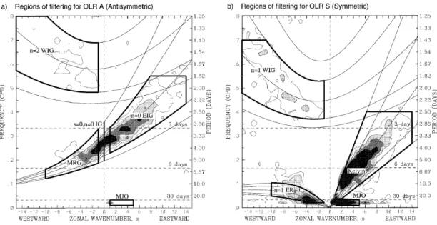
Wheeler and Kiladis [1999] found that the equatorial outgoing longwave radiation (OLR) power had spectral signatures that were significantly above the background at certain wavenumber-frequency domain regions, matching with the dispersion curves of the different equatorial wave types and the MJO, as shown in Fig. 2.3 from their paper.

Our method to filter waves is similar to that of Wheeler and Kiladis [1999], but analyzes

temperature and N

at all levels between 10-35 km altitude instead of OLR. For filtering, the

data must be periodic in longitude and time and cover all longitudes of the equatorial latitude

Fig. 2.3 Regions of the wavenumber-frequency domain with power spectrum above the background, thin contours starting at 1.1 and shading above 1.2. (a) antisymmetric component, (b) symmetric component of the OLR spectrum. The wave dispersion curves are for equivalent depths h = 8, 12, 25, 50 and 90 m. Thick-lined boxes indicate the regions of the wavenumber-frequency domain used for filtering. Figure from Wheeler and Kiladis [1999].

regular longitude grid on a daily basis. The filter settings are fairly similar to those shown in Fig. 2.3, although we allow for larger equivalent depths to account for the faster and not convectively coupled waves modes that can exist near the tropopause and throughout the stratosphere.

At a certain latitude band, and for each vertical level (0.1 km vertical spacing), the data consists of a longitude-time array, which is detrended and tapered in time. Then, a space-time bandpass filter is applied using a two-dimensional Fast Fourier Transform. This is done using the freely available ’kf-filter’ NCL function [Schreck, 2009].

The Fast Fourier Transform separates, in the longitude direction, all the zonal structure of temperature anomalies into a sum of harmonics of different wavenumbers. The same is done in the time dimension: each wavenumber has to oscillate in time with a certain frequency within the region defined for the bandpass filter, in order to be captured by it. If waves are present, which are theoretically defined by space-time harmonics, their filtered signal is outstanding compared to the (unavoidable to filter) background noise, which appears as a continuum of low-amplitude fluctuations [Wheeler and Kiladis, 1999].

Combining the filtered signals of each vertical level, which are filtered independently, will

explained next.

2.3.2 Extratropics

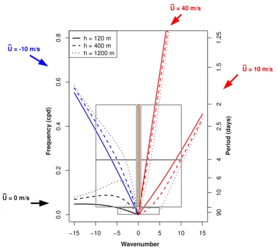
The extratropical wave modes differ greatly from those at the equator: they are not equa- torially trapped and can propagate in any direction, the Coriolis parameter has to be taken into account since it is non-zero outside the equator, and the zonal wind regimes in the extratropics are much more variable than the equatorial ones. Background winds affect the propagation of waves, by Doppler-shifting their dispersion relations or even precluding their propagation, therefore it is of special importance to take them into account in the extratropics.

We make a comparison of the dispersion curves of the extratropical Rossby wave under different background zonal wind regimes in Figure 2.4. The Rossby wave dispersion relation is defined as the most common form of large-scale wave disturbance found in the extratropics:

a planetary wave forced from the troposphere, and propagating vertically and zonally in a quasi-geostrophic flow. Assuming N

and background mean zonal winds ( ¯U) to be constant, and no meridional propagation for simplicity, the following dispersion relation can be obtained (following Andrews et al. [1987], see chapter for Linear Wave Theory):

w = s U ¯ − sβ [s

+ f

/gh]

where w is the frequency, s is the zonal wavenumber, f the Coriolis parameter, β its meridional derivative at a certain latitude (the Beta-plane approximation), g the gravity acceleration and h the equivalent depth. Since we assume no meridional propagation for simplicity, the meridional wavenumber is set to zero so it is absent in this formula (compared to Andrews et al. [1987]). The term (s ¯U) accounts for the Doppler-shifting of the dispersion relation by the background zonal winds; and the (f

/gh) term is an approximation to account for the vertical propagation of the wave.

Figure 2.4 shows how the dispersion curve of a Rossby wave changes depending on its equivalent depth (different line types), and the background zonal mean winds (zero winds black, blue for easterlies, red for westerlies, see specific arrows outside the diagram). Note that each dispersion curve is not valid for the entire year for the Rossby wave, only for the seasons with similar background ¯U.

The dispersion relations in Fig. 2.4 show the difficulty of defining a wave type in the

extratropics: the dispersion curve for a given wave type (idealized Rossby wave in this case)

can be in every possible place within the wavenumber-frequency domain, depending on the

U = 0 m/s

U = 10 m/s U = ­10 m/s

Wavenumber

Frequency (cpd) Period (days)

Fig. 2.4 Examples of dispersion curves for forced planetary waves at 50°N under different mean zonal wind regimes (line colors, winds specified outside the diagram), and differentiating equivalent depths (line type, top-left box). Filter bounds in the wavenumber-frequency domain are shown as grey boxes (brown for wavenumber zero). Figure from Pilch Kedzierski et al. [2016b].

that is valid for the entire time period (2007-2013) and that could be used at all levels between 5 and 35 km altitude.

Instead of defining certain dispersion curves, we use wide boxes in the wavenumber- frequency domain, only differentiating eastward-westward propagating oscillations with respect to the ground and their periods (faster 2-4 day waves; slower 4-25 day waves; and 30-96 day or quasi-stationary waves), which are displayed as the six grey boxes in Fig. 2.4.

We also define a seventh filter for wavenumber zero (s = 0, brown box in the middle of the diagram in Fig. 2.4) for completeness. This way, the Rossby waves will be captured by one or another filter, independently of the background zonal winds.

With this method we prioritize knowing the total effect of planetary and synoptic-scale

study targets TIL modulation and enhancement by extratropical waves, and not to disclose particular properties of these waves.

The space-time filtering methodology has never been applied to extract extratropical waves before due to the variability of background zonal winds which precludes defining a specific dispersion curve for the waves. By simplifying the methodology, the novel procedure developed during the doctoral work, as explained within this subsection, allows the extraction of the combined signal from planetary and synoptic-scale extratropical waves.

Next, sections 3, 4 and 5 will show the main results of this thesis, as reprints of the

scientific publications produced during the doctoral work.

3 The Tropical Tropopause Inversion Layer: Variability and Modulation by Equa- torial Waves

This chapter is a reprint of the article of the same name under review in Atmospheric Chemistry and Physics Discussions. It investigates the daily variability of the horizontal and vertical N

structures in the tropics, the relationship of stronger TIL with near-tropopause divergent flow, and how the QBO affects the TIL and also forms a secondary N

maximum below the zero-wind line.

The TIL modulation and enhancement by equatorial waves is quantified for the first time, comparing the relative roles of Kelvin, Rossby, IGWs and the MJO. Lastly, the remaining TIL without the equatorial wave signal is shown.

Citation:

Pilch Kedzierski, R., K. Matthes, and K. Bumke (2016a), The tropical tropopause inversion layer: variability and modulation by equatorial waves, Atmospheric Chemistry and Physics Discussions, pp. 1-31, doi:10.5194/acp-2016-178, (in review).

Author contributions to this publication:

- R. Pilch Kedzierski initiated the study, designed the method, did the analysis, produced all the figures and wrote the manuscript.

- K. Matthes contributed with ideas and discussions on the analysis, and commented the manuscript.

- K. Bumke contributed with ideas and discussions on the analysis, and commented the

manuscript.

Manuscript prepared for Atmos. Chem. Phys.

with version 2015/04/24 7.83 Copernicus papers of the L^ATEX class copernicus.cls.

Date: 28 July 2016

The Tropical Tropopause Inversion Layer: Variability and Modulation by Equatorial Waves

Robin Pilch Kedzierski

, Katja Matthes

, and Karl Bumke

1Marine Meteorology Department, GEOMAR Helmholtz Centre for Ocean Research Kiel, Kiel, Germany.

2Faculty of Mathematics and Natural Sciences, Christian-Albrechts-Universität zu Kiel, Kiel, Germany.

Correspondence to:Robin Pilch Kedzierski (rpilch@geomar.de) Abstract.

The Tropical Tropopause Layer (TTL) acts as a ’transition’ layer between the troposphere and the stratosphere over several kilometers, where air has both tropospheric and stratospheric properties.

Within this region, a fine-scale feature is located: the Tropopause Inversion Layer (TIL), which consists of a sharp temperature inversion at the tropopause and the corresponding high static stability 5

values right above, which theoretically affect the dispersion relations of atmospheric waves like Rossby or Inertia-Gravity waves and hamper stratosphere-troposphere exchange (STE). Therefore, the TIL receives increasing attention from the scientific community, mainly in the extratropics so far.

Our goal is to give a detailed picture of the properties, variability and forcings of the tropical TIL, with special emphasis on small-scale equatorial waves and the QBO.

10

We use high-resolution temperature profiles from the COSMIC satellite mission, i.e.∼2000 mea- surements per day globally, between 2007 and 2013, to derive TIL properties and to study the fine- scale structures of static stability in the tropics. The situation at near tropopause level is described by the 100hPa horizontal wind divergence fields, and the vertical structure of the QBO is provided by the equatorial winds at all levels, both from the ERA-Interim reanalysis.

15

We describe a new feature of the equatorial static stability profile: a secondary stability maxi- mum below the zero wind line within the easterly QBO wind regime at about 20-25km altitude, which is forced by the descending westerly QBO phase and gives a double-TIL-like structure. In the lowermost stratosphere, the TIL is stronger with westerly winds. We provide the first evidence of a relationship between the tropical TIL strength and near-tropopause divergence, with stronger 20

(weaker) TIL with near-tropopause divergent (convergent) flow, a relationship analogous to that of TIL strength with relative vorticity in the extratropics.

To elucidate possible enhancing mechanisms of the tropical TIL, we quantify the signature of the different equatorial waves on the vertical structure of static stability in the tropics. All waves show, on average, maximum cold anomalies at the thermal tropopause, warm anomalies above, and a net 25

TIL enhancement close to the tropopause. The main drivers are Kelvin, inertia-gravity and Rossby

waves. We suggest that a similar wave modulation will exist at mid and polar latitudes from the extratropical wave modes.

1 Introduction

The Tropopause Inversion Layer (TIL) is a narrow region characterized by temperature inversion and 30

enhanced static stability located right above the tropopause. This fine-scale feature was discovered by tropopause-based averaging of high-resolution radiosonde measurements by Birner et al. (2002) and Birner (2006). Satellite Global Positioning System radio occultation observations (GPS-RO) show that the TIL is present globally (Grise et al., 2010).

Static stability is a parameter used in a number of wave theory approximations, thus affecting the 35

dispersion relations of atmospheric waves like Rossby or Inertia-Gravity waves (Birner, 2006; Grise et al., 2010). Also, static stability suppresses vertical motion and correlates with sharper trace gas gradients, inhibiting the cross-tropopause exchange of chemical compounds (Hegglin et al., 2009;

Kunz et al., 2009; Schmidt et al., 2010). For these reasons, the TIL attracts increasing interest from the scientific community.

40

There is a considerable body of research about the TIL in the extratropics, establishing the TIL as an important feature of the extratropical upper-troposphere and lower-stratosphere (Gettelman et al., 2011). In the tropics, the transition between the troposphere and the stratosphere is considered to happen over several kilometers, dynamically and chemically (Fueglistaler et al., 2009; Gettelman and Birner, 2007), but less is known about the tropical TIL, as the following review will show.

45

In the extratropics, climatological studies have shown that the TIL reaches maximum strength during polar summer (Birner, 2006; Randel et al., 2007; Randel and Wu, 2010; Grise et al., 2010), whereas the TIL within anticyclones in mid-latitude winter is of the same strength or even higher from a synoptic-scale point of view (Pilch Kedzierski et al., 2015). Several mechanisms for ex- tratropical TIL formation/maintenance have been studied: water vapor radiative cooling below the 50

tropopause (Randel et al., 2007; Hegglin et al., 2009; Kunz et al., 2009; Randel and Wu, 2010), dynamical heating above the tropopause from the downwelling branch of the stratospheric residual circulation (Birner, 2010), tropopause lifting and sharpening by baroclinic waves and their embedded cyclones-anticyclones (Wirth, 2003, 2004; Wirth and Szabo, 2007; Son and Polvani, 2007; Randel et al., 2007; Randel and Wu, 2010; Erler and Wirth, 2011), and the presence of small-scale gravity 55

waves (Kunkel et al., 2014). A high-resolution model study by Miyazaki et al. (2010a, b) suggests that radiative effects dominate TIL enhancement in polar summer whereas dynamics are the main drivers in the remaining latitudes and seasons.

On the other hand, very little research has focused on the tropical TIL. Bell and Geller (2008) showed the TIL from one tropical radiosonde station, and Wang et al. (2013) reported a slight weak- 60

ening of the tropical TIL between 2001-2011. Grise et al. (2010) included the horizontal and vertical

variability of the tropical TIL in their global study about near-tropopause static stability, which is so far the most detailed description of the TIL in the tropics. They found the strongest TIL centered at the equator in the layer 0-1km above the tropopause, peaking during NH winter. This agrees well with the seasonality and location of tropopause sharpness as described later by Son et al. (2011) and 65

Kim and Son (2012). The horizontal structures in seasonal mean TIL in the tropics are reminiscent of the equatorial stationary wave response associated with climatological deep convection (Grise et al., 2010; Kim and Son, 2012). Grise et al. (2010) also noted that static stability is enhanced in the layer 1-3km above the tropopause during the easterly phase of the quasi-biennial oscillation (QBO).

Equatorial waves influence the intraseasonal and short-term variability of the temperature struc- 70

ture near the tropical tropopause (Fueglistaler et al., 2009). Kelvin waves and the Madden-Julian oscillation (MJO) (Madden and Julian, 1994) were reported as the dominant modes of temperature variability at the tropopause region (Kim and Son, 2012). Equatorial waves cool the tropopause re- gion (Grise and Thompson, 2013), and also produce a warming effect above it (Kim and Son, 2012).

This wave effect forms a dipole that can sharpen the gradients that lead to TIL enhancement, but no 75

study has quantified this effect so far.

Our study aims to describe the tropical TIL, its variability and forcings in detail, in order to increase the knowledge about its properties and highlight this sharp and fine-scale feature within the tropical transition layer between the troposphere and the stratosphere. Section 2 will show the datasets and methods used in our analyses. Section 3 will describe the vertical and horizontal struc- 80

ture and day-to-day variability of the TIL, its relationship with near-tropopause divergence, and the influence of the QBO on the vertical structure of static stability and TIL strength in particular. In section 4 we quantify the signature of the different equatorial waves and their effect on the mean temperature and static stability profiles in tropopause-based coordinates. Section 5 will discuss the applicability of our results with equatorial wave modulation to the extratropical TIL, given the dif- 85

ferent wave spectrum in the extratropics, and section 6 sums up the results.

2 Data and Methods 2.1 Datasets

We analyze temperature profiles from GPS radio occultation (GPS-RO) measurements which are provided at a 100m vertical resolution, from the surface up to 40km altitude, comparable to high- 90

resolution radiosonde data. Although the effective physical resolution of GPS-RO retrievals is of

∼1km, it improves in regions where the stratification of the atmosphere changes, such as the tropopause and the top of the boundary layer, i.e. the vertical resolution is highest where it is most needed (Kursinski et al., 1997). The advantage of GPS-RO is based on its global coverage, high sampling density of∼2000 profiles/day, and weather-independence. We mainly use data from the COSMIC 95

satellite mission (Anthes et al., 2008) for the years 2007-2013. For Figure 1 only, we added two ear-

lier GPS-RO satellite missions: CHAMP (Wickert et al., 2001) and GRACE (Beyerle et al., 2005), which provide less observations (around 200 profiles/day together) for 2002-2007.

The situation at near-tropopause level is retrieved from the ERA-Interim reanalysis (Dee et al., 2011). We make use of horizontal wind divergence and geopotential height fields at 100hPa on a 100

2.5°×2.5° longitude-latitude grid and 6-hourly time resolution, and also daily-mean vertical profiles of the zonal wind at the equator, for the time period 2007-2013. We choose the 100hPa level because it is the standard pressure level from ERA-Interim that is closest to the climatological tropopause in the tropics (96-100hPa in summer, 86-88hPa in winter, Kim and Son (2012)). Tropical winds near the tropopause in ERA-Interim differ from observations slightly more than in the extratropics, 105

but still are of good quality (Poli et al., 2010; Dee et al., 2011), and the variability of horizontal divergence is in balance with temperatures, which are constrained by GPS-RO in the UTLS.

2.2 TIL Strength Calculation

We define the tropopause height (T P_z) using the WMO lapse-rate tropopause criterion (WMO, 1957). Given the strong negative lapse-rate found above the tropopause near the equator, the lapse- 110

rate tropopause nearly coincides with the cold-point tropopause most of the time. This is in agree- ment with earlier studies, which did not find substantial differences in their results applying different tropopause definitions (Grise et al., 2010; Wang et al., 2013). From the GPS-RO temperature pro- files, vertical profiles of static stability are calculated as the Brunt-Väisälä frequency squared (N² [s⁻²]):

115

N²= (g/Θ)·(∂Θ/∂z)

where g is the gravitational acceleration, andΘthe potential temperature. Profiles with unphys- ical temperatures orN²values (temperature <-150°C, >150°C orN² >100×10⁻⁴s⁻²) and those where the tropopause cannot be found have been excluded. TIL strength (sTIL) is calculated as the maximum static stability value (N_max² ) above the tropopause level. This sTIL measure is commonly 120

used (Birner et al., 2006; Wirth and Szabo, 2007; Erler and Wirth, 2011; Pilch Kedzierski et al., 2015), because it makes sTIL independent of its distance from the tropopause andN²is a physically relevant quantity. Our algorithm searches forN_max² in the first 3km aboveT Pz, but most often finds it in the first kilometer.

2.3 Mapping of TIL Snapshots 125

The procedure to derive daily TIL snapshots in this study is similar to the method by Pilch Kedzierski et al. (2015), but with a longitude-latitude projection.

The daily TIL snapshots were estimated at a 5° longitude-latitude grid between 30°S-30°N. For each grid point we calculate the meanN_max² from all GPS-RO profiles within +-12.5° longitude-

latitude to account for the lower GPS-RO observation density in the tropics compared to the extrat- 130

ropics (Son et al., 2011). This setting avoids gaps appearing in the maps, and smooths out undesired small-scale features that cannot be captured with the current GPS-RO sampling.

We also produce similar maps of 100hPa horizontal wind divergence. For a fair comparison with the TIL snapshots, we equal the spatial scale and follow the same method, but instead of averaging N_max² values, we use the collocated divergence of each GPS-RO profile: the value from the nearest 135

ERA-Interim grid point and 6h time period to each observation. Examples of TIL snapshots can be found in Figure 2 (section 3.1.2). If plotted at full horizontal resolution, divergence would show small-scale features superimposed over the synoptic-to-large scale structures in Fig. 2, making the comparison withN_max² more difficult.

2.4 Wavenumber-Frequency Domain Filtering 140

Our purpose is to extract the temperature andN²signature of the different equatorial wave types on the zonal mean vertical profiles. For this, we follow Wheeler and Kiladis (1999), that studied equato- rial wave signatures on the outgoing longwave radiation (OLR) spectrum observed from satellites by wavenumber-frequency domain filtering. Wheeler and Kiladis (1999) give an in-depth description of the theoretical and mathematical background of the filtering methods.

145

Theoretically, the equatorial wave modes are the zonally and vertically propagating, equatorially trapped solutions of the ’shallow water’ equations (Matsuno, 1966; Lindzen, 1967) characterized by four parameters: meridional mode number (n), frequency (v), zonal planetary wavenumber (s) and equivalent depth (h). Each wave type (Kelvin, Rossby, the different modes of Inertia-Gravity waves) has a unique dispersion curve in the wavenumber-frequency domain, given its modenand equivalent 150

depthh.

Wheeler and Kiladis (1999) found that the equatorial OLR power had spectral signatures that were significantly above the background. The signature’s regions in the wavenumber-frequency domain match with the dispersion curves of the different equatorial wave types. Also, they found signatures outside of the theoretical wave dispersion curves that have characteristics of the Madden-Julian 155

oscillation (MJO) (Madden and Julian, 1994).

Our method is similar to that of Wheeler and Kiladis (1999), but analyzes temperature andN² at all levels between 10-35km altitude instead of OLR. For filtering, the data must be periodic in longitude and time and cover all longitudes of the equatorial latitude band. Therefore, the COSMIC GPS-RO profiles (Anthes et al., 2008) need to be put on a regular longitude grid on a daily basis. We 160

explain how this is done in the follwing section (2.4.1). More details about our proceeding with the filter, and the differences from Wheeler and Kiladis (1999) can be found in section 2.4.2. Note that this method is only used in Figs. 5 and 6 (section 4).