Asymmetric shockwave collisions in AdS 5

JHEP08(2019)005

Published for SISSA by Springer

Received: June 25, 2019 Accepted: July 24, 2019 Published: August 1, 2019

Asymmetric shockwave collisions in AdS ₅

Sebastian Waeber,

Andreas Rabenstein,

Andreas Sch¨ afer

and Laurence G. Yaffe

aInstitute for Theoretical Physics, University of Regensburg, D-93040 Regensburg, Germany

bDepartment of Physics, University of Washington, Seattle WA 98195-1560, U.S.A.

E-mail: sebastian.waeber@physik.uni-regensburg.de, andreas.rabenstein@physik.uni-regensburg.de,

andreas.schaefer@physik.uni-regensburg.de, yaffe@phys.washington.edu

Abstract: Collisions of asymmetric planar shocks in maximally supersymmetric Yang- Mills theory are studied via their dual gravitational formulation in asymptotically anti-de Sitter spacetime. The post-collision hydrodynamic flow is found to be very well described by appropriate means of the results of symmetric shock collisions. This study extends, to asymmetric collisions, previous work of Chesler, Kilbertus, and van der Schee examining the special case of symmetric collisions [1]. Given the universal description of hydrodynamic flow produced by asymmetric planar collisions one can model, quantitatively, non-planar, non-central collisions of highly Lorentz contracted projectiles without the need for comput- ing, holographically, collisions of finite size projectiles with very large aspect ratios. This paper also contains a pedagogical description of the computational methods and software used to compute shockwave collisions using pseudo-spectral methods, supplementing the earlier overview of Chesler and Yaffe [2].

Keywords: AdS-CFT Correspondence, Holography and quark-gluon plasmas, Quark- Gluon Plasma, Gauge-gravity correspondence

ArXiv ePrint: 1906.05086

JHEP08(2019)005

Contents

1 Introduction and summary 1

2 Planar shock collisions in asymptotically AdS spacetime 5

2.1 Characteristic formulation 5

2.2 Solution strategy 8

2.3 Planar shocks 9

3 Computational methods and software construction 12

3.1 Transformation to infalling coordinates 12

3.2 Horizon finding 16

3.3 Time evolution 17

4 Results 20

4.1 Calculated collisions 20

4.2 Hydrodynamic flow 20

5 Discussion 28

A Einstein equations for planar shocks 29

B Transformation to infalling coordinates 31

B.1 Near-boundary expansions 33

C Pseudo-spectral methods 35

C.1 Explicit expressions 37

C.2 Domain decomposition 38

D Filtering 38

D.1 Longitudinal filter 38

D.2 Radial filter 39

E Runge-Kutta methods 40

1 Introduction and summary

Despite the fact that QCD is not conformal, supersymmetric, or infinitely strongly coupled,

and has only a small number (N = 3) of colors, the comparison of heavy ion phenomenology

with predictions based on AdS/CFT duality (of “holography”) has turned out to be quite

fruitful [1–16]. At temperatures above the QCD phase transition the lack of supersym-

metry is of minor importance and effects caused by the other differences can be described

JHEP08(2019)005

perturbatively, either on the QCD or gravity side of the duality. For example, corrections due to large but finite values of the ’t Hooft coupling λ = g

N relevant for QCD can be calculated perturbatively on the gravity side, while the effects of non-conformality can be studied within QCD either perturbatively or using lattice gauge theory. Hence, it has been possible to identify which results from holographic modeling of heavy ion collisions should be more, or less, applicable to real QCD. Examples of observables with relatively modest corrections due to finite coupling and non-conformality effects include the viscos- ity to entropy density ratio [18], 4πη/s = 1 + 15 ζ(3) λ

≈ 1.4 for λ ≈ 12, and the short hydrodynamization time predicted by AdS/CFT duality based on calculations of the lowest quasinormal mode (QNM) frequency [19]. For the latter quantity, finite coupling corrections are larger than for η/s, but not so much as to change the picture qualitatively.

In this paper we study the hydrodynamic flow resulting from asymmetric collisions of planar shocks in strongly coupled, maximally supersymmetric Yang-Mills theory. Our work extends previous work on planar shock collisions [2, 3, 6, 11, 14] and, in particular, the observation by Chesler, Kilbertus, and van der Schee of “universal” flow with simple Gaussian rapidity dependence in the special case of symmetric collisions of planar shocks [1].

For such symmetric collisions, the authors of ref. [1] found that on a post-collision surface of constant proper time lying within the hydrodynamic regime, τ = τ

& τ

≈ 2/µ, the fluid 4-velocity is very well described by boost invariant flow,

u

= 1 , u

= u

= 0 , (1.1)

(with ds

≡ −dτ

+ τ

dξ

+ dx

), while the proper energy density is well described by a Gaussian in spacetime rapidity,

(ξ, τ

) = µ

A(µw) e

. (1.2) This proper energy density is defined as the timelike eigenvalue of the rescaled stress- energy tensor,

T b

≡ 2π

N

T

, (1.3)

so T b

u

= − u

. The energy scale µ characterizes the transverse energy density of each incoming shock and is defined by the longitudinally integrated (rescaled) energy density of either incoming shock,

µ

≡ Z

dz T b

(z ± t)

. (1.4) The longitudinal width w of the incoming shocks is defined as the energy density weighted rms width [1]. For the specific choice τ

= 3.5/µ, ref. [1] found

A(µw) ≈ 0.14 + 0.15 µw − 0.025 (µw)

, (1.5a) σ(µw) ≈ 0.96 − 0.49 µw + 0.13 (µw)

. (1.5b) For studying asymmetric planar shock collisions, we choose to work in the center-of- momentum (CM) frame in which the transverse energy densities of the incoming shocks are equal,

µ ≡ µ

= µ

. (1.6)

JHEP08(2019)005

In this frame the two incoming shocks will have widths w

and w

, and physical results may now depend on two independent dimensionless combinations which we take to be µw

and µw

.

Over a substantial range of incoming shock widths {w

, w

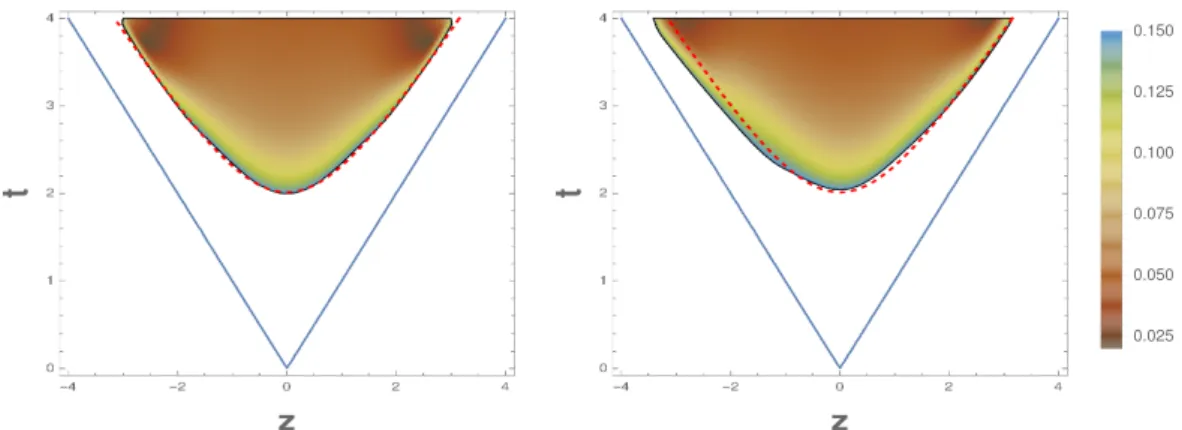
} ranging from 0.35/µ down to 0.075/µ, we find that the spacetime region in which hydrodynamics is applicable has little or no dependence on the shock widths, or their asymmetry, and is sensitive only to the initial energy scale µ. Using the same definition of a hydrodynamic residual and the 15% figure of merit chosen in ref. [1], we find that the boundary of the hydrodynamic region of validity remains at

µ t

≈ 2 , (1.7)

even for highly asymmetric collisions.

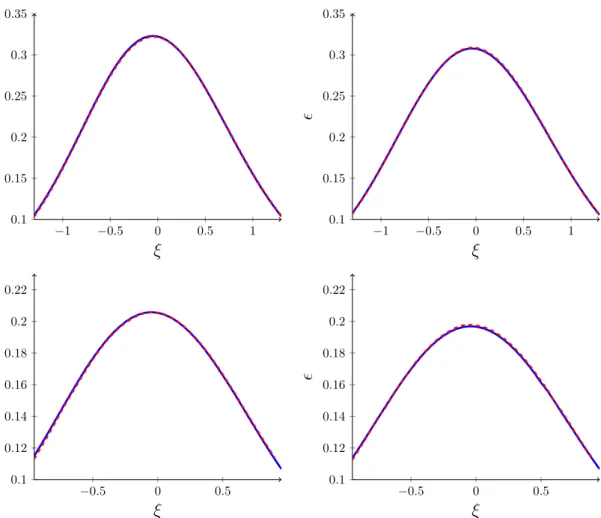
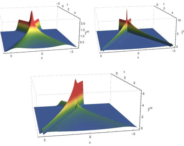
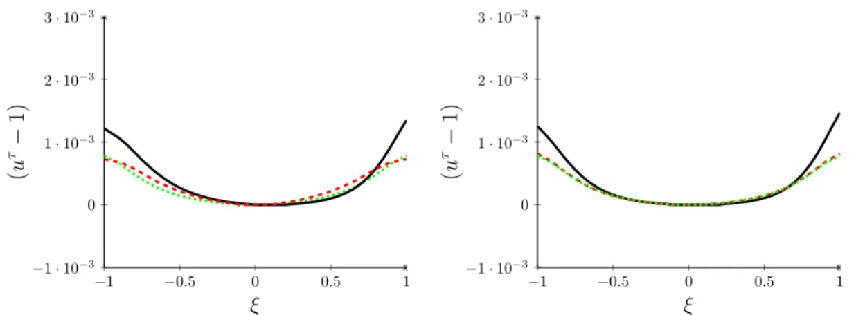
Similarly, the fluid 4-velocity resulting from asymmetric collisions remains very close to ideal boost invariant flow (1.1), while the post-collision proper energy density remains well-described by a Gaussian. However, the amplitude A, mean ¯ ξ, and width σ of the Gaussian rapidity dependence are now functions of both incoming shock widths,

(ξ, τ

) = µ

A(µw

, µw

) e

. (1.8) For asymmetric collisions, the outgoing energy density peaks at a non-zero mean rapidity ξ ¯ which is well-described by

ξ(µw ¯

, µw

) ≈ Ξ w

− w

w

+ w

, (1.9)

where the coefficient Ξ is constant for τ > 2 (as shown below in figure 6) and has the value Ξ ≈ 7 × 10

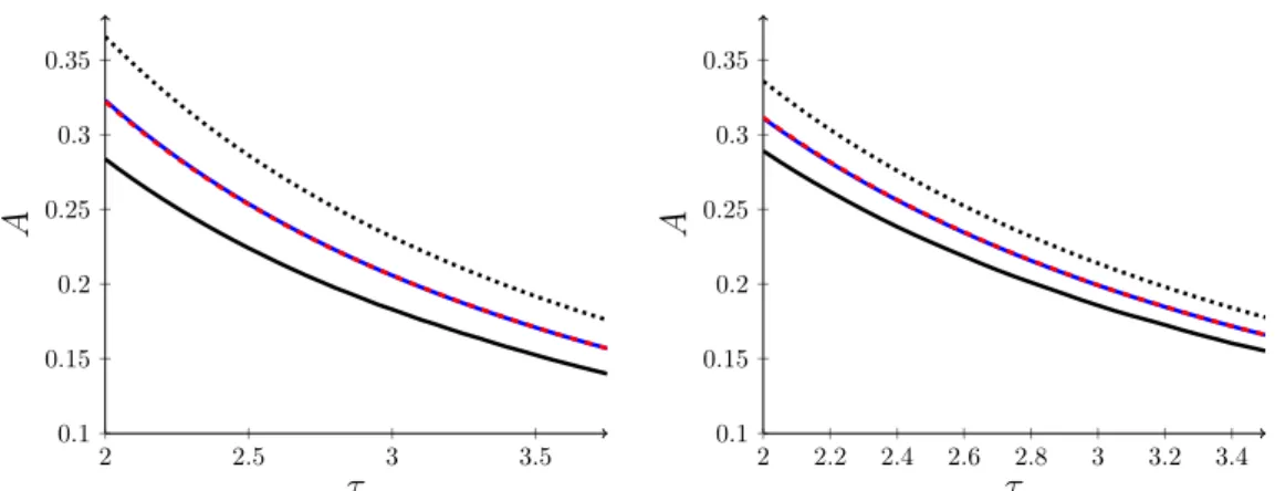
. We find that the amplitude A is well-described by the geometric mean of the symmetric collision results,

A(µw

, µw

) ≈ p

A(µw

) A(µw

) . (1.10)

In fact, after shifting the rapidity by ¯ ξ, we find that the geometric mean of the full sym- metric collision rapidity distributions provides a good approximation to the asymmetric collision results. For the width of the rapidity distribution, this implies that

σ(µw

, µw

) ≈ 1

2 σ(µw

)

+ 1

2 σ(µw

)

. (1.11)

For asymmetric collisions, the fit to the data provided by the this Gaussian model is good, as may be seen below in figure 7, but is not quite as perfect as for symmetric collisions. A more elaborate model, discussed in section 4.2, involves a weighted geometric mean of the symmetric collision profiles and provides an even better description, valid over a wider range of rapidity.

Given the above extension of the “universal” flow resulting from planar shock collisions

to the asymmetric case, we now have the ingredients needed to predict initial conditions for

the hydrodynamic flow resulting from collisions of bounded projectiles with finite transverse

extent, provided the transverse size of the incident projectiles is large compared to their

JHEP08(2019)005

(Lorentz contracted) longitudinal widths, so that spatial gradients in transverse directions are small compared to longitudinal gradients. The following algorithm provides the leading term in an expansion in transverse gradients:

• Regard the colliding system as composed of independent subregions in the transverse plane, or “pixels”, with each pixel having a size δ ≡ 1/Q

which is small compared to the transverse extent of the projectiles, but large compared to their longitudinal widths.

• Let j label independent transverse-plane pixels, with p

(j) the portion of the longi- tudinal momentum of each incident projectile residing within pixel j.

• For each pixel j, transform to the CM frame in which the total longitudinal mo- mentum within the pixel vanishes, and evaluate the resulting energy scale µ(j) and incident projectile widths w

(j) for this pixel. Explicitly, µ(j)

= 4 p

(j) p

(j)/δ

.

• Use the planar shock results (1.1), (1.8)–(1.11), plus the constitutive relation for a conformal fluid (4.2), to construct each pixel’s stress-energy tensor T

(j) at the initial proper time τ

.

• Transform each pixel’s stress-energy tensor T

(j) from its CM frame back to the original (lab) frame.

The result is a representation of the full system’s stress-energy tensor on the τ

initial surface, with transverse variation on the pixel scale δ, suitable for use as initial data for further hydrodynamic evolution. This procedure uses strongly coupled holographic dynamics to map energy density profiles of the initial projectiles, which may include initial state fluctuations and have non-vanishing impact parameter, into hydrodynamic initial data, without the need to perform full 5D numerical relativity calculations which are very challenging [8]. As noted above this procedure, based on planar shock results, should be viewed as the first term in an expansion in (small) transverse gradients. It would, of course, be interesting to derive, systematically, subsequent terms in this expansion.

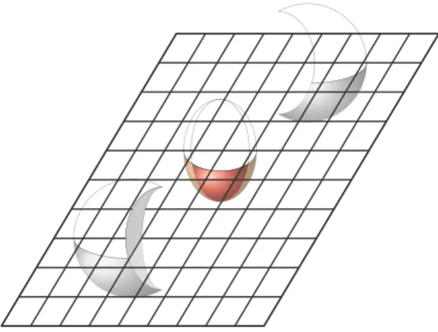
Pixels near the periphery of the overlap region of colliding nuclei, illustrated in figure 1, will have decreasing CM frame transverse energy density µ

due to the rapid fall-off of the transverse energy density of the colliding nuclei near their periphery. Given the fact that the hydrodynamization time scales inversely with µ (1.7), this implies that pixels near the periphery of the overlap region (shown in orange) will enter the hydrodynamic regime much later than pixels in the middle of the overlap region.

How this impacts an appropriate choice of the initial Cauchy surface used in hydrodynamic modeling, and the resulting uncertainties in estimates of, for example, the elliptic flow parameter v

, is deserving of further study.

1When transforming from the CM frame back to the lab frame, the hydrodynamization time thydro

is nearly Lorentz invariant. More precisely, as discussed in section 4.2 and in ref. [1], the boundary of the hydrodynamic regime is well-described as a Lorentz invariant hyperboloid relative to an origin with a modest temporal displacement.

JHEP08(2019)005

Figure 1. Sketch of a peripheral heavy ion collision. The almond shaped overlap region forms a quark-gluon plasma, not the spectator portions (shown in grey). The hydrodynamization time increases rapidly as one approaches the boundary of the overlap region, whose shape influences the value of the experimentally measured elliptic flow parameter v2.

The remainder of this paper is organized as follows. In section 2 we review the char- acteristic formulation of general relativity in asymptotically anti-de Sitter spacetimes and the initial data for planar shock collisions, largely following ref. [2]. Section 3 describes the numerical procedure and software used to compute shock collisions, highlighting several issues in greater detail than in ref. [2]. Results are presented in section 4, followed by a brief final discussion in section 5. Readers primarily interested in results should feel free to turn directly to section 4. Additional computational details are presented in the appendix.

2 Planar shock collisions in asymptotically AdS spacetime

2.1 Characteristic formulation

As shown in refs. [2–4, 8, 17], the characteristic formulation of general relativity, origi- nally developed by Bondi and Sachs [20, 21], provides a computationally effective method for handling the diffeomorphism invariance of general relativity when studying collisions dynamics in asymptotically AdS spacetimes.

The characteristic formulation is based on a null slicing of the geometry in which coordinates are directly tied to a congruence of null geodesics. We will use X ≡ (x, r) to denote 5D coordinates, with x = (x

, x

) ≡ (t, x

) representing ordinary Minkowski coordinates on the boundary of the AdS spacetime. Requiring that t = const. surfaces be null hypersurfaces implies that the one-form k = ∇ t is null, 0 = k

k

= g

k

k

, which means that g

= 0. Requiring the spatial coordinates x

to be constant along the null rays tangent to k

implies that 0 = k

∂

x

= g

(∂

t)(∂

x

), which means that g

= 0. These conditions on the contravariant components of the metric then imply that g

= g

= 0. Hence, under these assumptions the most general line element may be written in the generalized infalling (or Eddington-Finkelstein) form,

ds

= 2dt

β(X) dr − A(X) dt − F

(X) dx

+ G

(X) dx

dx

. (2.1)

JHEP08(2019)005

It will be convenient to factor the spatial metric G

into a scale factor Σ times a unimodular matrix b g,

G

(X) ≡ Σ(X)

b g

(X) , (2.2)

with det( b g) ≡ 1. One may fix one further condition, controlling the parameterization of the null geodesics tangent to k

. Bondi and Sachs [20, 21] chose to fix the scale factor Σ(X) = r, convenient for problems with spherical symmetry. We instead follow Chesler and Yaffe [2] and choose to set

β(X) = 1 . (2.3)

This condition leaves a residual reparametrization invariance in the metric (2.1) consisting of radial shifts,

r → r ˜ = r + δλ(x) , (2.4)

with the shift δλ depending in an arbitrary fashion on the boundary coordinates x. Under such a shift, the metric coefficient functions transform as

A(x, r) → A(x, e ˜ r) ≡ A(x, r−δλ) + ˜ ∂

δλ(x) , (2.5a) F

(x, r) → F e

(x, r) ˜ ≡ F

(x, r−δλ) + ˜ ∂

δλ(x) , (2.5b) G

(x, r) → G e

(x, r) ˜ ≡ G

(x, r−δλ) ˜ . (2.5c) From these transformations of A and F

it is apparent that they may be regarded as temporal and spatial components of a gauge field representing radial shifts. It is possible to write the Einstein equations in a manner which is manifestly covariant under radial shifts. To do so, it is convenient to define modified temporal and spatial derivatives,

d

≡ ∂

+ A(X) ∂

, d

≡ ∂

+ F

(X) ∂

. (2.6) Given these definitions, the Einstein equations,

R

− 1

2 R g

+ Λ g

= 0 , (2.7)

acquire a nested structure with the schematic form,

∂

+ Q

[ g] b

Σ = 0 . (2.8a)

δ

∂

+ P

[ b g, Σ]

∂

+ Q

[ b g, Σ]

F

= S

[ b g, Σ]

. (2.8b)

∂

+ Q

[Σ]

d

Σ = S

[ b g, Σ, F ] . (2.8c)

δ

δ

∂

+ Q

bg

[ b g, Σ]

d

b g

= S

bg

[ b g, Σ, F, d

Σ]

. (2.8d)

∂

A = S

[ b g, Σ, F, d

Σ, d

g] b . (2.8e)

δ

∂

+ Q

[ b g, Σ]

d

F

= S

[ b g, Σ, F, d

Σ, d

g, A] b

. (2.8f) d

(d

Σ) = S

+Σ

[ b g, Σ, F, d

Σ, d

b g, A] , (2.8g)

JHEP08(2019)005

Each equation is a first or second order linear radial differential equation for the indicated metric component(s) or their modified time derivatives. The square brackets of each coeffi- cient or source function indicates on which fields the term depends. Explicit form of these equations, for the case of planar shocks, are given in appendix A.

Given the rescaled spatial metric b g on any time slice, plus suitable boundary con- ditions, each radial differential equation may be integrated in turn, thereby determining both the other metric coefficients and the time derivative of g b on that time slice. The required boundary conditions may be inferred from the near-boundary behavior which can be obtained by solving equations (2.8a)–(2.8g) order by order in r. One finds [2],

A = 1

2 (r+λ)

− ∂

λ + a

r

+ O(r

) , F

= −∂

λ + f

r

+ O(r

) , (2.9a) Σ = r+λ + O(r

) , b g

= δ

+ b g

r

+ O(r

) , (2.9b) d

Σ = 1

2 (r+λ)

+ a

r

+ O r

, d

b g

= −2 b g

r

+ O(r

) . (2.9c) The coefficients a

, f

and b g

cannot be determined by a local near-boundary analysis.

Note that b g

is necessarily traceless (because b g has unit determinant). These coefficients are mapped, via gauge/gravity duality, to the stress-energy tensor of the dual field theory.

In our infalling coordinates this relation is given by [2]

2π

N

hT

i ≡ T b

= h

+ 1

4 h

η

, (2.10) with h

≡ −2a

, h

≡ −f

, and h

≡ b g

. Here N

is the number of colors in the dual field theory, and η = diag(−1, +1, +1, +1) is the Minkowski metric tensor. Explicitly,

T b

= − 3

2 a

, T b

= −f

, T b

= b g

− 1

2 a

δ

. (2.11) The radial shift parameter λ(x) is completely undetermined in expansion (2.9) and may be chosen arbitrarily. As in previous work [2–4, 8, 17], we use this freedom to set the radial position r

(x) of the apparent horizon equal to a fixed value,

r

(x) = r

. (2.12)

It is sufficient to solve for the spacetime geometry in the region between the horizon and the boundary because information hidden behind the horizon cannot propagate outward and influence boundary observables. Thus, the choice (2.12) results in a convenient rectangular computational domain.

With our metric ansatz (2.1), demanding a fixed radial position of the apparent horizon

leads to a condition on d

Σ [2]. To derive this condition, one may write the tangents to

a radial infalling null congruence in the form k

(X) = µ(X) ∇

φ(X) for some scalar

functions φ and µ. Demanding that the one-form k be null allows one to reexpress the

time derivative of φ in terms of spatial derivatives. Requiring that the congruence satisfy

the (affinely parameterized) geodesic equation k

k

= 0 allows one to reexpress the time

JHEP08(2019)005

derivative of the multiplier function µ in terms of its spatial derivatives. Given these time derivatives, one may then compute the expansion θ = ∇ · k on the time slice of interest.

Demanding that the expansion vanish on a surface φ(X) = const. implies that this surface is an apparent horizon. Applying this procedure to the metric ansatz (2.1) and specializing to the case φ(X) = r leads to the desired condition [2],

d

Σ

= − 1

2 (∂

Σ) F

− 1

3 Σ ∇ · F . (2.13)

This condition must hold at all times if the radial position of the horizon is to remain fixed at some given value r

. Consequently, on every time slice the condition

∂

d

Σ

= ∂

− 1

2 (∂

Σ)F

− 1

3 Σ ∇ · F

(2.14) is also required to hold. When combined with the Einstein equation (2.8g), this final condition leads to an elliptic differential equation for the value of the metric function A on the (apparent) horizon. Explicit forms of the horizon equation (2.13) and the horizon stationarity condition (2.14) may be found in appendix A.

2.2 Solution strategy

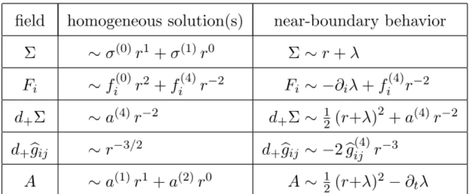
To solve the nested form (2.8) of the Einstein equations, one requires appropriate boundary data which picks out the correct solution for each equation. The needed boundary condi- tions are determined by the homogeneous solutions of each equation and the asymptotic behavior of the desired solutions. This information is summarized in table 1. From this table one sees that a choice for the radial shift λ along with values of the asymptotic coef- ficients a

and f

are needed as boundary conditions for the Σ, F

, and d

Σ equations and serve to fix the coefficient of a homogeneous solution to the corresponding differential equation. The asymptotic coefficients a

and f

, proportional to the boundary energy and momentum density, are dynamical degrees of freedom (in addition to the metric b g

) and are determined by integrating the stress-energy continuity equation as discussed below.

The radial shift λ(x) will also be treated as a dynamical degree of freedom, as described below, and adjusted in a manner which ensures that the apparent horizon remains at a fixed radial position.

Given this boundary data, together with the value of b g on some given time slice, the radial differential equations (2.8a)–(2.8d) may each be integrated in turn, at every spatial location x

, leading to a determination of d

g b

on the time slice. Two boundary conditions are needed to integrate the second order equation (2.8e) for the metric function A. As seen in table 1, the value of the radial shift λ supplies one condition. The second boundary condition is supplied by the value of A at the apparent horizon, which is determined by solving the horizon stationarity condition (2.14).

Having determined both d

b g and A, the actual time derivative for the rescaled spatial metric b g is then reconstructed as

∂

b g

= d

b g

− A ∂

b g

. (2.15)

JHEP08(2019)005

field homogeneous solution(s) near-boundary behavior Σ ∼ σ

r

+ σ

r

Σ ∼ r + λ

F

∼ f

r

+ f

r

F

∼ −∂

λ + f

r

d

Σ ∼ a

r

d

Σ ∼

(r+λ)

+ a

r

d

b g

∼ r

d

b g

∼ −2 b g

r

A ∼ a

r

+ a

r

A ∼

(r+λ)

− ∂

λ

Table 1. Near-boundary asymptotic behavior of the homogeneous solutions to the radial differential equations (2.8a)–(2.8e) for the indicated fields, together with the desired asymptotic behavior of physical solutions. The asymptotic coefficientsa⁽⁴⁾,f_i⁽⁴⁾, andbg_ij⁽⁴⁾determine respectively the energy density, momentum density, and traceless stress tensor of the dual field theory. The leading terms in the near-boundary behavior of all fields except Σ are driven by the inhomogeneous source terms in the various equations and do not correspond to homogeneous solutions.

Knowing d

Σ and A (on a given time slice), the near boundary expansion (2.9) shows that the time derivative of the the radial shift λ(x) may be extracted as

∂

λ = lim

r→∞

(d

Σ − A) . (2.16)

Similarly, the asymptotic coefficient g b

determining the traceless stress tensor is extracted from the boundary limit of either r

( g b

− δ

) or −

r

d

b g

. This information then allows one to determine the time derivatives of a

and f

using the boundary stress-energy continuity equation, ∇

hT

i = 0, which is an automatic consequence of the Einstein equations. Explicitly,

∂

a

= 2

3 ∂

f

, ∂

f

= 1

2 ∂

a

− ∂

b g

. (2.17) The above procedure, involving integration of a sequence of linear ordinary differential equations in the radial direction plus one spatial elliptic equation on the apparent horizon, determines the time derivatives of the dynamical data { b g

, λ, a

, f

} given initial values of this data on some time slice. These time derivatives are then input into a conventional time integrator, such as fourth order Runge-Kutta, to advance to the next time slice where the entire process repeats.

Overall, this characteristic formulation transforms the highly non-linear coupled Ein- stein equations into a set of nested linear ordinary differential equations and first order time evolution equations. We solve the radial differential equations, and the horizon stationarity equation, using spectral methods as described in some detail in section 3 and appendix C.

2.3 Planar shocks

By “planar shock” we mean an asymptotically anti-de Sitter solution of the vacuum Ein-

stein equations whose boundary stress-energy tensor describes a “sheet” of energy density

which moves at the speed of light in some longitudinal direction and is translationally

JHEP08(2019)005

invariant in the other two transverse spatial dimensions. For regular solutions, such a sheet of moving energy density will have some smooth longitudinal profile and non-zero characteristic thickness.

Let {x

} ≡ (x

, z) denote spatial coordinates separated into transverse and longitudi- nal components, and consider shocks moving in the ±z direction. To specialize the general infalling metric ansatz (2.1) to the case of planar shock spacetimes, we impose translation invariance in transverse directions plus rotation invariance in the transverse plane, which implies that all metric components are functions of only of r and x

≡ t ∓ z, that F

only has a longitudinal component, and that the (rescaled) spatial metric has the form [2],

b g = diag(e

, e

, e

) . (2.18) Consequently,

ds

= 2dt (dr − A dt − F

dz) + Σ

e

dx

+ e

dz

. (2.19)

The boundary asymptotics (2.9) implies that the “anisotropy” function B behaves as B(x

, r) = b

(x

) r

+ O(r

) . (2.20) For later computational convenience, let

u ≡ 1/r (2.21)

denote an inverted radial coordinate, so that the spacetime boundary lies at u = 0.

In general it does not seem possible to find analytic forms of planar shock solutions using the infalling Eddington-Finkelstein (EF) coordinates (2.19). But analytic solutions are available in Fefferman-Graham (FG) coordinates [3, 8, 24]. Using {˜ x

, ρ} ≡ { ˜ ˜ t, x ˜

, z, ˜ ρ} ˜ as our FG coordinates, with ˜ x

≡ ˜ t ± z ˜ and ˜ ρ an inverted bulk radial coordinate, the metric

ds

= ˜ ρ

−d˜ x

d˜ x

+ d˜ x

+ d˜ ρ

+ ˜ ρ

h(˜ x

) d˜ x

, (2.22) is a planar shock solution describing a shock moving in the ±z direction with arbitrary longitudinal energy density profile h(z). In the calculations described below, we use simple Gaussian profiles with width w and longitudinally integrated energy density µ

,

h(z) ≡ µ

(2πw

)

e

. (2.23) The associated boundary stress-energy tensor is just

T b

(˜ t, z) = ˜ T b

(˜ t, z) = ˜ ± T b

(˜ t, z) = ˜ h(˜ t−˜ z) , (2.24) with all other components vanishing.

Focusing, for ease of presentation, on shocks moving in the +z direction, the transla- tional symmetries imply that the EF and FG coordinates will be related by a transformation of the form [2],

t ˜ = t + u + α(t−z, u) , z ˜ = z − γ(t−z, u) , ρ ˜ = u + β(t−z, u) , (2.25)

and ˜ x

= x

.

JHEP08(2019)005

As discussed above, the required initial data for the characteristic evolution scheme consists of the anisotropy function B plus the boundary data {a

, f

} and the radial shift λ. Inserting a transformation of the form (2.25) into the FG metric (2.22), a short exercise [2] shows that

B = − 1 3 ln

− (∂

α)

+ (∂

β )

+ (1 − ∂

γ )

+ (u + β)

(1 − ∂

α − ∂

γ )

h

, (2.26) while the boundary data is given by

a

= − 2

3 h , f

= h , λ = − 1 2 ∂

β

. (2.27)

To solve for the transformation functions {α, β, γ}, one approach, used in refs. [2, 3], is to insert the transformation (2.25) into the FG metric (2.22) and demand that the result have the EF form (2.19).

To simplify the resulting equations, it is helpful to redefine the transformation functions α and β via

α = −γ + β + δ , β = − u

ζ

1 + uζ . (2.28)

One finds [2] that the functions ζ and δ satisfy a pair of coupled differential equations, 1

u

∂

∂u

u

∂ζ

∂u

+ 2uH

(1 + uζ)

= 0 , ∂δ

∂u − u

(1 + uζ)

∂ζ

∂u = 0 , (2.29a)

while γ satisfies a decoupled equation,

∂γ

∂u − u

(1 + uζ)

∂ζ

∂u + u

2(1 + uζ)

∂ζ

∂u

+ u

H

2(1 + uζ)

= 0 , (2.29b) with H ≡ h + t − z + u + δ − u

ζ/(1 + uζ)

. The desired solutions have the near- boundary behavior

ζ ∼ λ + O(u

) , δ ∼ O(u

) , γ ∼ O(u

) . (2.29c) Integrating equations (2.29) with boundary conditions ensuring the behavior (2.29c), and inserting the resulting transformation functions into eqs. (2.26) and (2.27), yields the anisotropy function B and associated boundary data describing of a single shock.

To construct initial data for colliding shocks, we superpose counter-propagating single shock data at an initial time t

when the two shocks are sufficiently widely separated that their overlap is negligible,

B(u, z, t

) = B

(u, t

−z) + B

(u, t

+z) , (2.30a) a

(z, t

) = a

(t

−z) + a

(t

+z) , (2.30b) f

(z, t

) = f

(t

−z) − f

(t

+z) . (2.30c)

2An alternative approach, used in ref. [8] for more general metrics, is based on observing that the curve defined by fixed values of the EF boundary coordinates and all values of r,X^A(r) = (t0, xⁱ₀, r), is a null geodesic of the EF metric (2.1) withr an affine parameter. Therefore the same path in FG coordinates, Ye(X(r)), will satisfy the geodesic equation ^d2_dr^Ye₂^A +Γ(Ye )^A_BC^deY_dr^{B dY}_dr^eC = 0 with eΓ^A_BC denoting the FG coordinate Christoffel symbols. Explicit forms of the resulting equations can be found in appendixB.

JHEP08(2019)005

However, unlike for the other functions, the overlap of the radial shifts λ

of the left and right moving shocks in the region close to z = 0 is significant. Since we choose the shocks on the first time slice to be well separated, we may regard the geometry in between as deviating negligibly from pure AdS. This justifies modifying the initial shift function λ in the neigh- borhood of z = 0, without changing the physical data {B(u, z, t

), a

(z, t

), f

(z, t

)}.

As in ref. [2], we adjust the initial radial shift by setting

λ(z, t

) = θ

(−z) λ

(t

−z) + θ

(z) λ

(t

+z) , (2.31) with θ

(z) ≡

1 − erf(−z/( √ 2w

))

a smoothed step function.

In practice, we slightly modify the above superposition procedure. Following refs. [2, 3], we replace eq. (2.30b) with

a

(z, t

) = a

(t

−z) + a

(t

+z) − 2

3

. (2.32)

From the form (2.11) of the stress-energy tensor, one sees that

is a constant additive shift in T b

. In other words,

is an (artificial) uniform background energy density. Adding a small background energy density helps alleviate numerical problems, as discussed below, and physically means that the colliding shocks will be propagating through a background thermal medium. If the background energy density

is sufficiently small compared to the energy densities in the colliding shocks, then the background will effectively be very cold (compared to the energy scale µ of the shocks) and there will be little dissipation to the medium. This modification is done purely for numerical convenience and we will be interested in results extrapolated to vanishing background energy density.

3 Computational methods and software construction

The aim of this section is to describe the construction of a planar shockwave collision code in sufficient detail so that an interested reader could create their own version with relatively modest effort. Those primarily interested in results should skip to the next section.

3.1 Transformation to infalling coordinates

As explained in ref. [2] and the previous section, the transformation from Fefferman- Graham to infalling coordinates may be computed by first solving for the congruence of infalling geodesics in FG coordinates. Or, in the special case of planar shock geometries, one can directly solve the simplified transformation equations (2.29). We implemented both approaches, and found them to have comparable numerical efficiency. Here, we focus on the direct approach of solving eqs. (2.29) for the case of a right moving shock. Henceforth, for convenience, we also set µ = 1. Appropriate factors of µ can always be reinserted via dimensional analysis.

We solve the coordinate transformation equations (2.29) in the rectangular region u ∈ [0, u

], z ∈ [−L

/2, L

/2] using Newton-Raphson iteration (i.e., linearizing each equation in the deviation of the solution from the current approximation), and solving the resulting linear equations using spectral methods with domain decomposition.

3A good introduction to spectral methods may be found in, for example, ref. [22].

JHEP08(2019)005

Periodic boundary conditions are imposed in the longitudinal direction and functions of z are approximated as truncated Fourier series. This is exactly equivalent to characterizing any function f(z) by a list of its values, {f

≡ f (z

)}, on an evenly spaced Fourier grid composed of N

points,

z

≡ L

− 1

2 + l/N

, (3.1)

for k = 0, · · ·, N

−1. Derivatives with respect to z turn into the application of a Fourier grid differentiation matrix D

= k(D

)

k applied to the vector of function values,

f

(z

) = X

l

(D

)

f

. (3.2)

Explicit expressions for the Fourier grid differentiation matrix components (D

)

are given in appendix C. A rather fine longitudinal grid is required to accurately represent thin shocks within a large longitudinal box. We used Fourier grids with N

= 960 for L

= 12 and shock widths down to 0.075.

To represent the dependence of functions on the radial coordinate u we first decompose the domain [0, u

] into M equally sized subdomains, and then use a Chebyshev-Gauss- Lobatto grid with N

points within each subdomain. This amounts to using a radial grid composed of the points

u

≡ u

2M

2j − 1 − cos πk N

−1

, (3.3)

for j = 1, · · ·, M and k = 0, · · ·, N

−1. The radial dependence of some function g(u) is represented by the list of M × N

function values on this grid, {g

≡ g(u

)}, and derivatives with respect to u turn into the application of a (block diagonal) Chebyshev differentiation matrix D

applied to this list of function values,

g

(u

) = X

l

(D

)

g

. (3.4)

Explicit expressions for the components of the Chebyshev differentiation matrix D

are given in eq. (C.12). As discussed in ref. [2], using domain decomposition (i.e., M > 1) helps to avoid excessive precision loss in the numerical evaluation of equations near the u = 0 boundary, and allows the use of a larger time step without running afoul of CFL instabilities. To integrate radial equations down to u

= 2, we used radial grids with up to M = 22 domains and N

= 12 points within each subdomain.

The product of these 1D grids defines our 2D spectral grid. Any function f (u, z) becomes a set of N

≡ M × N

× N

values on these grid points,

{f

≡ f (u

, z

)} . (3.5)

Fortunately, the differential equations (2.29) are completely local in z. So these equations,

evaluated on the 2D grid with derivatives replaced by the corresponding differentiation

matrices, do not become a single set of 2N

(for eq. (2.29a)) or N

(for eq. (2.29b))

coupled algebraic relations. Rather they yield N

decoupled systems, each involving 2M N

(for eq. (2.29a)) or M N

(for eq. (2.29b)) variables.

JHEP08(2019)005

For each set of equations, linearization around some initial, or current, guess for a solution leads to a set of linear equations of the generic form M f = −S, where f is the unknown vector of function deviations from the current guess, S is the vector of residu- als, and M is the spectral approximation to the linear operator which results from the linearization of the differential equation (s) at some given value of z.

At this point, these linear equations are singular. First, u = 0 is a regular singular point of the differential equations (2.29a) and (2.29b); one cannot simply evaluate, numerically, these equations at u = 0. Moreover, solutions to these differential equations are, of course, non-unique. One must complement the differential equations with suitable boundary con- ditions to specify a unique solution. With spectral methods, fixing one of these problems fixes the other. Prior to linearization, one simply replaces the (ill-defined) evaluation of the equations at u = 0 by constraints encoding required boundary conditions.

Examining equations (2.29a) and (2.29b), one sees that the most general near-boundary behavior is

ζ ∼ ζ

u

+ λ + O(u

) , γ ∼ γ

+ O(u

) , δ ∼ δ

+ O(u

) , (3.6) for arbitrary values of the coefficients ζ

, λ, γ

and δ

. We want to set the leading coefficients ζ

, γ

and δ

to zero. To implement this Dirichlet condition for γ and δ in a manner which avoids unnecessary precision loss when computing derivatives of these functions at the boundary, it is convenient first to redefine

γ(z, u) ≡ u

γ(z, u) ˜ , δ(z, u) ≡ u

δ(z, u) ˜ , (3.7) and then reexpress equations (2.29) in terms of ˜ γ and ˜ δ. Unwanted solutions with non- zero boundary values for γ or δ are then simply not representable when using our spectral representation for ˜ γ or ˜ δ. Similarly, using our spectral representation for ζ automatically eliminates unwanted solutions where ζ has singular 1/u behavior.

The continuum differential equations imply that ˜ γ and ˜ δ both vanish, and have van- ishing first derivatives, at the boundary. To deal with the u = 0 regular singular point in the discretized equations for ˜ γ and ˜ δ it is sufficient to replace the equations at u = 0 with constraints setting ˜ γ and ˜ δ to zero. If we wished to fix the radial shift λ by simply specifying its value, we could similarly redefine ζ = λ + u ζ ˜ and require ˜ ζ to vanish at the boundary. However, we found it more convenient to fix λ indirectly by demanding that ζ vanish at our chosen value of u

. Referring to eqs. (2.25) and (2.28), one sees that this condition will make the u = u

surface coincide with a surface of constant FG radial coordinate, ˜ ρ = u

. In other words, with this condition the FG computational domain

˜

ρ ∈ [0, ρ ˜

] is the same as the EF domain u ∈ [0, u

].

The net effect of the above procedure, in the discretized equations for ζ, ˜ δ and ˜ γ at longitudinal position z

, is to replace the the (degenerate) equations at u = 0 by the respective constraints

ζ

= 0 , δ ˜

= 0 , γ ˜

= 0 . (3.8)

4Although not required, we also replaced a second row in the linearized equation forζ by the condition that the first derivative of ζ vanish on the boundary, P

j(Du)0jζ1,j,l = 0. The continuum equations automatically imply this behavior, but imposing it explicitly in the discretized equations helped to minimize precision loss associated with unwanted solutions that diverge on the boundary.

JHEP08(2019)005

In addition to applying boundary conditions at u = 0, when using domain decomposi- tion one must also impose continuity conditions at subdomain boundaries. Our set (3.3) of radial grid points redundantly duplicates the interior endpoints of each subdomain, u

= u

for j = 1, · · ·, M −1, and hence two different rows of the linear equa- tion Mf = −S represent the differential equation evaluated at the same physical point.

One could deal with this by eliminating the duplication of subdomain endpoints and suit- ably redefining the differentiation matrix D

. But it is even easier to fix the problem by simply replacing one of the rows representing an interior subdomain endpoint with a constraint equation enforcing the equality of duplicated function values at this point, f

− f

= 0.

After these row replacements, the modified linear system is reasonably well conditioned and, with a sufficiently good initial guess, Newton iteration rapidly converges quadratically.

To generate an initial guess, it is natural to work sequentially in z. If the shock is prop- agating in the +z direction with the profile function h(z) having its maximum at z = 0, then at the furthest point behind the shock, z

= −L

/2, the geometry deviates negligibly from pure AdS and ζ = ˜ γ = ˜ δ = 0 is a fine initial guess. Thereafter, we use the converged solution at each z

as an initial guess for the solution at z

. This provides a good initial guess provided the longitudinal grid spacing is sufficiently fine.

The above procedure for solving the transformation equations (2.29) using spectral methods works well as long as the radial depth u

to which one integrates is not too large. The key advantage of this approach is that the precision of the obtained solutions do not degrade near the boundary, even through u = 0 is a singular point of the differential equations. That is to say, spectral methods are excellent for finding well-behaved solutions of equations having regular singular points. However, as u

increases the linear operators one inverts in this Newton iteration scheme become increasingly ill-conditioned. Unfor- tunately, the depth to which one must integrate in order to locate the apparent horizon (discussed next) after superposing shocks grows with increasing separation of the initial shocks. We used two strategies to cope with this difficulty.

First, following refs. [2, 3], we added a small artificial background energy density

when superposing shocks as described above. Increasing the background energy density decreases the depth at which an apparent horizon forms. Second, after using the above approach to find the transformation functions for u < u

, we integrate further into the bulk by switching to an adaptive 4th order Runge-Kutta integrator, with the spectral solution at u

providing initial data. (A description of this standard integrator is given in appendix E.) For simplicity, we choose to integrate to a fixed value u = u

, instead of a fixed value of ˜ ρ.

For our chosen range of shock parameters, with widths down to w = 0.075, using a spectral grid down to u

= 2 worked well. With a longitudinal box size L

= 12 and

5There is a subtlety involving the choice of which row to replace as, relative to a given interior subdomain endpoint, one row approximatesuderivatives using information on one side of the endpoint, while the other row approximatesuderivatives using information on the other side. Since the behavior of the transformation functions is fixed, and known, at theu= 0 boundary, one should regard the transformation equations (2.29) as describing the propagation of information from the boundary into the bulk. Consequently, one should retain the row corresponding touj,N_u−1 and replace the row corresponding touj+1,0.

JHEP08(2019)005

background energy densities in the range of 1–5% of the peak energy density, it turned out that only a modest further integration with the adaptive integrator down to u

= 2.11 was sufficient to reach the apparent horizon throughout the longitudinal box.

Having transformed a right-moving single shock solution to infalling coordinates, and extracted the resulting initial data {B

, a

, f

, λ

} for evolution using eqs. (2.26)–(2.27), a simple reflection generates corresponding data for a left-moving shock,

B

(u, z) = B

(u, −z) , a

(z) = a

(−z) , (3.9a) λ

(z) = λ

(−z) , f

(z) = −f

(−z) . (3.9b) We construct initial data for counter-propagating shocks by combining single shock solutions as described earlier in eqs. (2.30)–(2.32). We chose the initial time t

for this superposition so that the initial separation between the shocks, ∆z

= −2t

, is large compared to the shock widths. We used ∆z

= 4 for symmetric collisions of broad shocks,

∆z

= 2 for symmetric collisions of thin shocks, and ∆z

= 3 for asymmetric collisions of shocks.

For thin shockwave collisions with small background energy density, avoiding numerical instabilities associated with short wavelength perturbations is challenging. As discussed in ref. [2], it is helpful to damp discretization induced perturbations using appropriate filtering.

We constructed and applied smoothing filters to the initial data in both longitudinal and radial directions. Details of these filters are presented in appendix D.2.

3.2 Horizon finding

After transforming chosen single shock solutions to infalling coordinates, as just discussed, and combining two counter-propagating shocks as shown in eqs. (2.30)–(2.32), the final step in the construction of initial data is locating the apparent horizon which serves as an IR cutoff in the bulk.

In our planar shock geometries, the apparent horizon condition (2.13) becomes 0 = d

Σ + e

6Σ

3F

∂

Σ + 2Σ ∂

F + 4F Σ ∂

B + 2F ∂

Σ

. (3.10)

A radial shift, r = ¯ r + δλ, corresponds in our inverted radial coordinates to u = u ¯

1 + ¯ u δλ . (3.11)

6For the parameters which we chose, displayed in table2and discussed below in section4, it turned out that using an adaptive integrator to probe deeper into the bulk was not essential, as the apparent horizon was found to lie within the domain of integration reached with spectral methods. However, as we used a relaxation algorithm to find the horizon, it was convenient to have additional surplus depth available, especially for small values of 0, since on some early iteration steps the current guess for the apparent horizon would lie deeper than the final value, possibly beyond the spectral solution endpoint.

7One subtlety is that the transformation to infalling coordinates is only computed to some finite depth umax. For a given configuration of initial shocks and chosen value of the background energy density0, it is a matter of trial and error to find a value of umax for the transformation which is sufficiently deep so that the apparent horizon lies above this depth, for all values ofz within the computational domain. The required value ofumaxincreases with the size of the longitudinal domain and separation of the initial shocks.

JHEP08(2019)005

If ¯ u ∈ [0, u

] represents the radial coordinate used in the transformation to infalling coordinates, then we wish to determine the value of a further shift δλ(z) such that con- dition (3.10) holds at some value of u

≡ 1/r

which may, for convenience, be chosen to equal the same value u

from the coordinate transformation. With this choice, δλ must be negative for the sought-after apparent horizon to lie within the coordinate transforma- tion domain.

Equation (3.10) is a nonlinear but ordinary differential equation for the shift function δλ(z). To solve it, we use spectral methods (with the same Fourier grid in z) combined with a root finding routine. Linearizing equation (3.10) in δλ allows us to apply Newton iteration. Each iteration step starts with a trial value of the radial shift, δλ

in iteration m, and computes the residual (i.e., the right-hand side of eq. (3.10)) and its variation with respect to δλ, and solves the linearized equation to find an improved value δλ

of the shift.

To evaluate the residual and its variation, we first integrate eqs. (2.8a)–(2.8c), using the current value of B(z, u) and λ(z), to find the auxiliary functions Σ, F and d

Σ.

After each step we convert the spectral representation of B (z, u) to a new radial grid with grid points shifted according to eq. (3.11). To do so, we perform off-grid interpolation using a sum of Chebyshev cardinal functions [22] with coefficients given by the on-grid values of B(z, u).

For our settings of longitudinal box size and shock parameters, we found it advanta- geous to choose the initial guess δλ

to be 0.1. It was also helpful to start with a relatively large background energy density

of about 10% of the peak shock energy density, and then gradually decrease

during each iteration step until it reached the desired final value before Newton iteration convergence.

During time evolution, described next, solving the horizon stationarity condition (2.14) on each time step yields the time derivative of the radial shift thereby providing the in- formation needed to integrate λ forward in time. (The explicit form of eq. (2.14) for our planar shock geometries is given in eq. (A.4).) To prevent discretization errors from driving long term drift away from the desired horizon condition (3.10), we also directly recomputed the apparent horizon position every 10–100 time steps using the above iterative procedure.

3.3 Time evolution

As described above in section (2.2), the data on any time slice needed to integrate forward in time consists of {B (z, u), a

(z), f

(z), λ(z)}. To compute the time derivative of this data, we successively solve eqs. (2.8a)–(2.8e) as discussed earlier. Explicit forms of these equations are given in eqs. (A.2a)–(A.2e) of appendix A. We use the same multi-domain spectral methods described above in section 3.1. These methods presume that functions being represented by their values on the spectral grid are well behaved throughout the computational domain.

Our functions Σ and A have divergent near-boundary behavior,

8Explicit forms of these equations are shown in appendixA. After the first integration of these equations, one could thereafter use off-grid spectral interpolation to evaluate the radially-shifted auxiliary functions on the spectral grid. But it is just as easy to reintegrate eqs. (2.8a)–(2.8c) on every Newton iteration step.

9See, for example, ref. [22] for a good discussion of the connection between analyticity properties and convergence of spectral representations.