Traveling wave solutions of reaction-diffusion equations with x-dependent combustion type nonlinearities

equations with x-dependent combustion type nonlinearities

Dissertation

zur Erlangung des akademischen Grades

eines Doktors der Naturwissenschaften (Dr. rer. nat.)

Der Fakultät für Mathematik der Technischen Universität Dortmund

vorgelegt von

Sven Badke

im März 2016

Traveling wave solutions of reaction-diffusion equations with x-dependent combustion type nonlinearities

Fakultät für Mathematik

Technische Universität Dortmund

Erstgutachter: Prof. Dr. Ben Schweizer Zweitgutachter: Prof. Dr. Matthias Röger

Tag der mündlichen Prüfung: 27.04.2016

I would like to express my gratitude towards the people who supported me in creating this thesis in different ways.

First and foremost, I would like to thank my supervisor Prof. Dr. Ben Schweizer for introducing me to the field of partial differential equations and providing me with the opportunity and guidance to write this thesis.

My gratitude also belongs to the members and former members of Lehrstuhl I and the Biomathematics group at the TU Dortmund, including Prof. Dr. Matthias Röger, Jun.-Prof. Dr. Tomáš Dohnal, Priv.-Doz. Dr. Andreas Rätz, Dr. Agnes Lamacz, Dr.

Peter Furlan, Maik Urban and Saskia Stockhaus, for creating such a wonderful working atmosphere. I am particularly grateful to my friends and colleagues Lisa Helfmeier, Stephan Hausberg, Carsten Zwilling, Dr. Jan Koch, Dr. Tobias Kloos and Christian Kühbacher for their support and encouragement.

A special thanks goes to my friend Sebastian Schäfer for his support and encouragement and his assistance with the English language.

Finally, I want to thank my family, in particular my parents Manfred and Jutta Badke, my sister Sandra Karla and my grandmother Rita Henkemeyer. With their

unconditional love and support, they contributed a great deal to the creation of this

thesis.

1. Introduction 7

1.1. Traveling waves in homogeneous media . . . . 7

1.2. Traveling waves in periodic heterogeneous media . . . . 11

2. Main results 20 2.1. Setting of the problem and basic definitions . . . . 20

2.2. Main results . . . . 26

2.3. A critical discussion of the results of Xin . . . . 27

2.3.1. Xin’s main results . . . . 28

2.3.2. Xin’s proof of existence . . . . 28

2.3.3. Xin’s proof of monotonicity and uniqueness . . . . 38

3. Plan of proof 40 3.1. Existence . . . . 40

3.2. Monotonicity and uniqueness . . . . 44

4. Existence of traveling wave solutions: the (ε, b)-problem 46 4.1. Elliptic regularization or the (ε, b)-problem . . . . 46

4.1.1. Monotonicity and uniqueness of the (ε, b)-solution . . . . 46

4.1.2. Existence of the (ε, b)-solution . . . . 52

4.2. Bounds on the wavespeed c

. . . . 69

4.2.1. Lower bounds on the wavespeed . . . . 69

4.2.2. Upper bounds on the wavespeed . . . . 73

5. Analysis of limits ε → 0, b → ∞ 81 5.1. Preparations for passing to the limit . . . . 81

5.1.1. Returning to (t, x) coordinates . . . . 81

5.1.2. A priori estimates for u

. . . . 82

5.2. Passage to the limit . . . . 91

5.2.1. Existence of the limit function u and its regularity . . . . 91

5.2.2. Possibilities for the values at infinity . . . . 98

5.2.3. The periodic principle eigenvalue and an exponential solution . . 102

5.2.4. Behavior of u at infinity . . . 110

5.2.5. The strict inequalities 0 < u < 1 and u

> 0 . . . 111

5.2.6. Conclusion of the existence proofs . . . 113

6. Monotonicity and uniqueness of traveling wave solutions 114 6.1. Minimum principles . . . 114 6.2. Proof of the monotonicity theorem 2.11 . . . 115 6.3. Proof of uniqueness theorem 2.12 . . . 118

A. Appendix 123

Bibliography 124

1.1. Traveling waves in homogeneous media

The notion of traveling waves in homogeneous media and typical nonlinearities

This work is concerned with traveling wave solutions to reaction-diffusion equations.

The basic form of a reaction-diffusion equation is

u

= ∆u + f(u) in (0, ∞) × R

. (1.1) According to [5], this equation was first introduced in the articles [10] of Fischer and [14] of Kolmogorov, Petrovsky and Piskunov in 1937 and 1938. The original motivation was to investigate the spreading of advantageous genes. The considered nonlinearities f were of logistic type, e.g. f (u) = u(1 − u) or f(u) = u(1 − u

). In both cases there are stationary states 0 and 1 of the equation.

A particular kind of solutions to the equation are traveling wave solutions or traveling front solutions. They can be imagined as front profiles, which connect the stationary states 0 and 1; the time-dependence is a shift into a direction k, |k| = 1, as t grows with a speed c. More exactly, this means that u is given by a pair (U, c), with a front profile U and a wavespeed c, such that u is of the form

u(t, x) = U (k · x − ct), (1.2)

0 ≤ U ≤ 1, U (−∞) = 0, U (+∞) = 1.

The direction k is given and the speed c is an unknown that is to be determined. In some cases there is a unique c, such that there exists a corresponding traveling wave solution (U, c). In other cases there are multiple c (for example an interval of the form (−∞, c

) or (−∞, c

]), such that there exist corresponding traveling wave solutions. The condition (1.2) on u can also be expressed as

u

t + k · v c , x + v

= u(t, x) for any vector v ∈ R

. (1.3) In case of space dimension one, this is perhaps more illustrative:

u

t + l c , x + l

= u(t, x) for any l ∈ R .

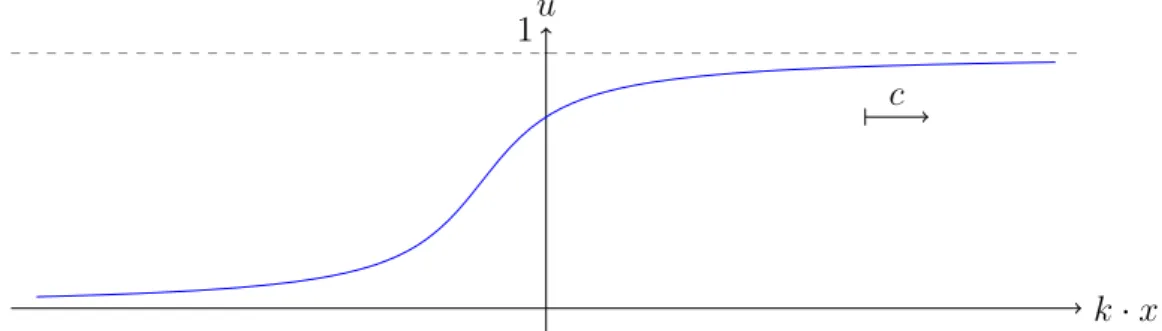
k · x u

c 1

Figure 1.1.: A qualitative view of a front profile in the homogeneous case.

−4 −2 0 2 4 −4 −2 0 2 4 0

0.5 1

k · x

t u(t, x)

Figure 1.2.: A qualitative picture of a traveling wave solution in the homogeneous case.

The ansatz u(t, x) = U(s) with s = k · x − ct is commonly called the moving frame ansatz. Inserting it into equation (1.1) leads to an ordinary differential equation for U :

U

= −cU

− f (U ). (1.4)

Among the usual questions are those of existence, uniqueness, monotonicity and stability of traveling wave solutions (U, c). Also of interest is the long term behavior of solutions to the initial value problem

u

= ∆u + f(u) in (0, ∞) × R

, u(0, x) = u

(x).

Of course, the results depend on the type of the nonlinearity f . As far as uniqueness is concerned, a traveling wave solution can only be unique up to a constant shift in s due to the shift-invariance of the equation in s. From (1.4), one can see that the space dimension is irrelevant in the questions of existence and uniqueness of traveling wave solutions.

In the overview article [17], Xin lists the following types of nonlinearities:

1. f(u) = u(1 − u) is called the KPP nonlinearity (after [14]) or Fisher nonlinearity (after [10]).

2. f(u) = u

(1 − u) with m ≥ 2, m ∈ N is called the m-th order Fisher nonlinearity or Zeldovich nonlinearity, if m = 2.

3. f(u) = u(1 − u)(µ − u) with µ ∈ (0, 1) is called the bistable nonlinearity.

4. f(u) = e

(1 − u) with activation energy E > 0 is called Arrhenius combustion nonlinearity or combustion nonlinearity with activation energy E but no ignition temperature cutoff.

5. f(u) = 0 in [0, θ] with θ ∈ (0, 1), f (u) > 0 in (θ, 1) and f (1) = 0, f Lipschitz continuous, is called a combustion nonlinearity with ignition temperature θ.

In [17], Xin also lists some of the fields in which these nonlinearities arise: Types 1 and 2 have their origin in chemical kinetics. Type 3 arises in biological applications. Types 4 and 5 arise in combustion science.

Some results in the homogeneous case

Let us first list some of the results, which are given in [17]: Let f be any of type 1 - type 5 in the above list with µ ∈ 0,

in case of type 3. By multiplying (1.4) with U

and integrating over R , it can be seen that

c = −

1

R

0

f(z) dz R

R

U

ds < 0. (1.5)

We want to explain this argument. By multiplying (1.4) with U

and integrating over an interval [a, b], one obtains

1

2 U

(b) − 1

2 U

(a) = −c

b

Z

a

U

(s) ds −

U(b)

Z

U(a)

f (z) dz.

For any fixed a ∈ R , the right hand side converges for b → ∞ to a value in R ∪{−∞, ∞}.

Therefore, the left hand side has to converge as well. It follows that, U

(b) → d for b → ∞ and some d ∈ [0, ∞] (since U

(b) ≥ 0). Consequently, U

(b) → ± √

d for b → ∞.

But then d = 0, because otherwise U (b) → 1 for b → ∞ cannot hold. By the same reasoning U

(a) → 0 for a → −∞. Therefore, one obtains

c

∞

Z

−∞

U

(s) ds = −

1

Z

0

f (z) dz < 0.

The left hand side cannot be 0, and one obtains (1.5). By this argumentation, one has also obtained U

(s) → 0 for s → ±∞.

We continue with the results given in [17]: It is often useful to rewrite the ordinary differential equation for U as a first order system

U

=: V,

V

= −cV − f(U ).

In this form, one can perform a phase plane analysis. A traveling wave solution of (1.1) corresponds to a trajectory in the (U, V ) plane connecting the points (0, 0) and (1, 0). For f of type 1, this method yields the existence of such a trajectory for every c ≤ c

= −2 p

f (0). In contrast, for f of type 3 with µ ∈ (0,

), there exists a unique trajectory for a unique c. In case of a type 2 nonlinearity f , there is c

such that there is a connecting trajectory for every c < c

.

For nonlinearities of types 4 and 5, Xin describes different methods involving degree theory. If f is of type 4, there is a c

, such that for every c < c

, there is a traveling wave solution (U, c). In case of a type 5 nonlinearity f, there is a unique traveling wave solution (U, c).

In the work [1], Aronson and Weinberger investigate the one dimensional reaction diffusion equation

u

= u

+ f(u). (1.6)

Their nonlinearity f is of the form f(u) = u(1 − u)((τ

− τ

)(1 − u) − (τ

− τ

)u). The parameters τ

, τ

and τ

stem from a biological model. This leads to three major cases and different relevant properties of f:

Case 1 τ

≤ τ

< τ

. Then f

(0) > 0, f (u) > 0 in (0, 1).

Case 2 τ

< τ

≤ τ

. Then f

(0) > 0, f

(1) > 0, f (u) > 0 in (0, α), f (u) < 0 in (α, 1) for some α ∈ (0, 1).

Case 3 τ

≤ τ

< τ

. Then f

(0) < 0, f(u) < 0 in (0, α), f (u) > 0 in (α, 1) for some α ∈ (0, 1),

1

R

0

f (u) du > 0.

Aronson and Weinberger examine the behavior of solutions of the initial boundary value problem on R

× R

and the pure initial value problem on R

× R and also the existence of traveling front solutions. For the results, we refer to the article [1].

In [9], Fife and McLeod treat the equation

u

= u

+ f (u) (1.7)

in one space dimension for a broad class of nonlinearities. In the existence part, it is

assumed that f ∈ C

[0, 1], f (0) = f (1) = 0 and for some α ∈ (0, 1) one of the following

three cases holds:

(a) f ≤ 0 in (0, α), f > 0 in (α, 1),

1

R

0

f(z) dz > 0.

(b) f < 0 in (0, α), f ≥ 0 in (α, 1),

1

R

0

f(z) dz < 0.

(c) f < 0 in (0, α), f > 0 in (α, 1).

In each of these cases, Fife and McLeod show the existence of traveling wave solutions.

They also investigate the asymptotic behavior of the initial value problem (1.7) on (0, ∞)× R , u(0, x) = φ(x) under similar conditions on f . If the initial values are pulselike and if there exists a traveling wave solution, the solution to the initial value problem converges exponentially to a shift of the traveling front solution. The exact result in the frontlike case is the following: Assume f ∈ C

[0, 1], f (0) = f (1) = 0, f

(0) < 0 and f

(1) < 0. Furthermore, assume f(u) < 0 for 0 < u < α

and f (u) > 0 for α

< u < 1, where 0 < α

≤ α

< 1. Suppose that there is a traveling wave solution (U, c). Let the initial values satisfy 0 ≤ φ ≤ 1 and lim sup

φ(x) < α

, as well as lim inf

φ(x) > α

. Then, for some constants z

, ω > 0 and K > 0, there holds

|u(t, x) − U (x − ct − z

)| < Ke

.

The result for pulselike initial values is of similar nature. Under similar assumptions on f as in the frontlike case and pulselike initial data, the solution u to the initial value problem converges exponentially to a shifted traveling wave solution for x < 0 and to a traveling wave moving in the opposite direction for x > 0. For the exact result in the pulselike case we refer to the article [9].

1.2. Traveling waves in periodic heterogeneous media

The notion of traveling waves in periodic heterogeneous media

We now consider the reaction-diffusion equation in a periodic heterogeneous medium.

A heterogeneous medium is modeled with x-dependent coefficients a

. We assume that (a

)

= (a

(x))

is a smooth, symmetric and uniformly elliptic matrix field, which is 1-periodic in every component of x. The periodicity can also be expressed by defining the matrix field on T

, the n-dimensional torus. Prototypes of the reaction-diffusion equation in heterogeneous media are

u

=

n

X

i,j=1

(a

(x)u

)

+ f (u) (divergence form) (1.8) and

u

=

n

X

i,j=1

a

(x)u

+ f (u) (non-divergence form). (1.9)

Of particular interest is the case where the nonlinearity f satisfies f(0) = f (1) = 0. In this case, the equations have the stationary states 0 and 1.

Neither for (1.8) nor for (1.9) we can expect to find a traveling wave solution of the form (1.2). Instead, the moving frame ansatz has to be extended. Consider the moving frame coordinates

s = k · x − ct, y = x. (1.10)

A (pulsating) traveling wave solution is a solution u given by a pair (U, c) with u(t, x) = U(s, y), 0 ≤ U ≤ 1,

U (s, ·) 1-periodic in each component of y,

s→−∞

lim U (s, y) = 0 and lim

s→∞

U (s, y) = 1 uniformly in y.



 

 

(1.11)

This can also be expressed without changing the coordinate system. A solution u of (1.8) or (1.9) (more precisely the pair (u, c)) is called a traveling wave solution if

0 ≤ u ≤ 1, u(t, x) = u

t + k · e

c , x + e

for the unit vectors e

, i = 1, ..., n,

t→−∞

lim u(t, x) = 0 and lim

t→∞

u(t, x) = 1 locally uniformly in x ∈ R

.

We emphasize that this description extends the formulation of (1.3). Of course, there are variants of the notion of a traveling wave solution. For example, other periodic lengths can be considered. The nonlinearity f might depend explicitly on x. The stationary states that are to be connected could be different from 0 and 1. The stationary states might even be nonconstant. Then, the notion of a traveling wave solution has to be properly adapted.

A prototypical result of Xin

We now come to a result of Xin [21], which is prototypical for our work. Consider the equation

u

=

n

X

i,j=1

a

(x)u

+ g(u). (1.12) The matrix (a

(x))

is smooth, positive definite and 1-periodic in every component of x ∈ R

. The nonlinearity g is a C

[0, 1] combustion nonlinearity.

Xin shows the existence of a traveling wave solution U of the form (1.11) with 0 <

U < 1 and U

> 0, as well as c < 0. The proof uses the method of elliptic regularization.

Under the additional assumption g

(1) < 0, Xin proves that every traveling wave solution

U satisfies the monotonicity U

> 0. Under the same assumption, he also proves the

uniqueness of (U, c) up to a constant shift in s. He uses the sliding domain method in the

proofs of both the monotonicity and the uniqueness result. Since our work is essentially

based on [21], we will discuss that article in more detail in chapter 2.

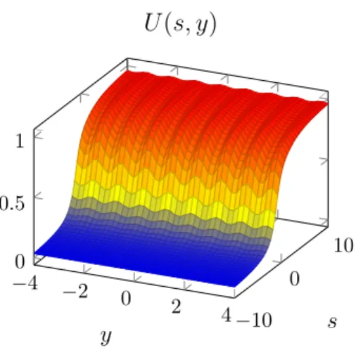
−4 −2 0 2 4 −10 0 0 10

0.5 1

y s

U (s, y)

Figure 1.3.: A qualitative view of a pulsating traveling wave solution in moving frame coordinates.

A review of results in the periodic heterogeneous case

A result from Xin which is similar to the previously discussed prototypical result is given in [18]. Consider the equation

u

=

n

X

i,j=1

(a

(x)u

)

+

n

X

i=1

b

(x)u

+ g (u).

It is assumed that (a

)

is a smooth, positive definite matrix field on T

. Moreover, (b

)

is a smooth vector field on T

, which is divergence free and has zero mean over T

. The function g is a combustion nonlinearity, which is C

in a neighborhood of 1 and satisfies g

(1) < 0.

Under these assumptions, Xin proves the existence of a traveling wave solution (U, c) with c < 0 and U strictly increasing in s. In the proof, he uses the method of con- tinuation. Under the same assumptions, Xin also shows the strict monotonicity of any traveling wave solution (if g ∈ C

[0, 1], even U

> 0) and the uniqueness of (U, c) up to constant shifts in s. As opposed to the case of equation (1.12), the condition g

(1) < 0 is also used in the existence part.

In [20], Xin examines the reaction diffusion equation in the form u

=

n

X

i,j=1

(a

(x)u

)

+

n

X

i=1

b

(x)u

+ f(x, u). (1.13)

It is assumed that the coefficients are smooth and 2π-periodic in every component of x ∈

R

. The matrix field (a

)

is assumed to be uniformly positive definite. Furthermore,

it is assumed to be a perturbation of the unit matrix: (a

(x))

= I + δ(˜ a

(x))

,

where (˜ a

)

is smooth and 2π-periodic in every component of x and δ is small. The

nonlinearity f is assumed to be a cubic bistable nonlinearity. For example, f(u) = u(1 − u)(µ − u) with µ ∈ (0,

). In the proofs, Xin assumes b

= 0 and that f does not depend on x.

In order to prove the existence of traveling wave solutions, he uses a perturbation ansatz: The case δ = 0 is the homogeneous case. For this case, the existence of a traveling wave solution (φ, c

) is known. Xin’s ansatz for a traveling wave solution (U, c) in moving frame coordinates is U = φ + δv and c = c

+ δc

. This leads to a problem for (v, c

), which we call the perturbation problem for the moment. After imposing an additional normalization condition, Xin obtains a unique solution v, if δ is sufficiently small. To obtain this solution, Xin uses methods of Fourier and spectral analysis.

More precisely, the result is as follows. Let k ∈ R

be a unit vector, m ∈ N

and m − [m/2] > (n + 1)/2. Consider the space

X

= {v ∈ H

( R × T

) : (∇

+ k∂

)

v ∈ H

( R × T

)}.

Then there exists δ

= δ

(c

, n, m) > 0, such that for δ < δ

, there exist unique v ∈ X

and c

∈ R , which solve the perturbation problem. Moreover, (U, c) = (φ + δv, c

+ δc

) is a traveling wave solution of (1.13). If (V, C) is another traveling wave solution of (1.13), then c = C and U (s − s

, y) = V (s, y) for some s

∈ R and (s, y) ∈ R × T

.

In [20], Xin also proves a stability result in space dimension one: Consider the equation u

= (a(x)u

)

+ f (u).

Xin assumes a(x) = 1 + δ˜ a(x), where ˜ a is a smooth and 2π-periodic function. Moreover, it is assumed that f (u) = u(1− u)(u −µ). For δ sufficiently small, there exists a traveling wave solution U of the equation, as Xin has proved in the existence part. Consider now the initial value problem

u

= (a(x)u

)

+ f (u), u(0, x) = U (x, x) + εu

(x).

The initial values are the perturbation of the traveling wave solution for t = 0. Xin’s stability result is as follows. Assume u

∈ H

( R ) and let u be the solution of the initial value problem. Assume further U ∈ C

( R ×T

) and U

∈ H

( R × T

). If ε is sufficiently small, there is a function γ = γ(ε) and a constant K = K(ρ

) for some ρ

∈ (0, 1) such that

||u(t, · + ct) − U (· + γ(ε), · + ct)||

≤ Kρ

for all t ≥ 0.

Moreover, γ(ε) = εh(ε), with a C

function h. Xin also gives a characterization of h(0) with an adjoint problem. For more details, we refer to [20].

In a two paper series [5] and [6], Berestycki, Hamel and Roques investigate a biolog- ical model for the persistence of species and propagation phenomena in a periodically fragmented environment model. The underlying equation is

u

= ∇ · (A(x)∇u) + f(x, u).

The function f(x, u) = u(µ(x) − ν(x)u) with a saturation coefficient ν and a growth rate µ is a prototypical example for the class of nonlinearities treated in [5].

In the first paper, the authors are concerned with the existence of a positive periodic stationary state p of the equation. Under appropriate assumptions on A and f , the existence of p is decided by the periodic principle eigenvalue of the linearized elliptic operator. The periodic principle eigenvalue is the unique λ

∈ R , such that there exists a periodic solution φ with φ > 0 of the equation

−∇ · (A(x)∇φ) − f

(x, 0)φ = λ

φ in R

.

If λ

< 0, the stationary state 0 is called unstable; in this case a stationary state p exists. If λ

≥ 0, then 0 is the only bounded stationary state. Under slightly different assumptions on f , it is shown that in the case λ

< 0, there exists at most one bounded positive stationary state.

The authors also consider solutions u to the initial value problem with certain non- trivial initial values. Under appropriate conditions, the authors show that in the case λ

< 0, the solution u(t, x) converges to p in C

( R

) as t → ∞ and in the case λ

≥ 0, u(t, x) converges to 0 as t → ∞.

In the second paper, the existence of traveling wave solutions is shown in the case that the stationary solution p exists. The proof uses an elliptic regularization method.

There are traveling wave solutions for a continuum of wave speeds c ≥ c

.

One can also study a domain Ω with Ω 6= R

which is periodic in some of the variables, namely in x = (x

, ..., x

), and bounded in the rest of the variables y = (x

, ..., x

).

Such a case is treated in the work [3]. In this article, the notion of a pulsating traveling wave solution has been carried over to the equation

u

− ∇

· (A(x, y)∇

u) + q · ∇

u = f (x, y, u).

Periodicity conditions are only imposed in x. Two types of nonlinearities f are treated.

We want to mention the first type, which is a combustion type with ignition temperature θ and a monotonicity condition in the vicinity of u = 1. This monotonicity condition is similar to g

(1) < 0 in [18], but less restrictive. For the precise results, we refer the reader to [3].

In [19], Xin is concerned with the asymptotic behavior of the initial value problem u

=

n

X

i,j=1

(a

(x)u

)

+

n

X

i=1

b

(x)u

+ f(u),

u(0, x) = u

(x), x ∈ R

.

It is assumed that (a

)

is a smooth, positive definite matrix field on T

. Moreover,

(b

)

is a smooth vector field on T

, which is divergence free and has zero mean over T

.

Two types of nonlinearities are treated, namely combustion nonlinearities and bistable

nonlinearities. The initial values u

are either frontlike or pulselike. What the terms frontlike and pulselike mean, depends on the nonlinearity. The asymptotic stability of pulsating traveling wave solutions are unclear. However, it can be shown in the case of frontlike data, that the solution to the initial value problem propagates with the speed of the traveling wave solution, if one exists. As an example, we sketch Xin’s result for the case of a bistable nonlinearity f (u) = u(1 − u)(µ − u) and frontlike data. Consider initial data 0 ≤ u

≤ 1. For a unit vector k ∈ R

, let S = {y ∈ R

: y = x − (k · x)k, x ∈ R

}.

The data u

are frontlike, if lim sup

k·x→−∞

u

(x) < µ and lim sup

k·x→+∞

u

(x) > µ

uniformly in S. Assume that a traveling wave solution (U, c(k)) exists. Then there exist smooth function ξ

= ξ

(t) and q

= q

(t), i = 1, 2, such that

U (k · x − c(k)t − ξ

(t), x) − q

(t) ≤ u(t, x) ≤ U(k · x − c(k)t + ξ

(t), x) + q

(t) for (t, x) ∈ R

. The functions ξ

and q

satisfy for i = 1, 2:

ξ

> 0, ξ

> 0, sup

t>0

|ξ

(t)| < +∞, q

> 0, q

≤ 0, q

(t) ≤ Ce

for some γ > 0. The results for pulselike data are similar but with a pair of traveling wave solutions U

and U

going in opposite directions. The results for combustion non- linearities are also similar. For the precise results, we refer to the article [19].

We want to mention a homogenization result by Heinze [13]. For ε > 0 he considers the equation

∂

u = ∇ · (A

(x)∇u) + 1

ε b

(x)∇u + f (u) for (t, x) ∈ R

. (1.14) It is assumed that A

(x) = A(

) with a matrix field A ∈ C

( R

; R

), which is sym- metric, elliptic and 1-periodic in every component of x. Furthermore, it is assumed that b

(x) = b(

) with a vector field b ∈ C

( R

; R

), which is 1-periodic in every component, divergence free and has zero mean over T

. The nonlinearity f is supposed to be a combustion nonlinearity as used in Xin [18]. The existence of a traveling wave solution in this setting has been established by Xin in [18] as described above. Heinze reasons that by the assumptions on b, there exists a skewsymmetric 1-periodic matrix B, such that with B

(y) = B(

), there holds ∇ · (B

∇u) =

b

∇u. He defines A ˜

:= A

+ B

, such that (1.14) becomes

∂

u = ∇ · ( ˜ A

(x)∇u) + f(u). (1.15)

The traveling wave solution (U

, c

) is given in moving frame coordinates s = k · x + c

t,

z =

, where c

> 0 is the wavespeed of the traveling wave solution. The function U

=

U

(s, z) is 1-periodic in every component of z and normalized by max

U (0, z) = θ.

Note that with these moving frame coordinates, the sign of the wavespeed is reversed in comparison to the moving frame ansatz (1.10). With ∇

:=

∇

+ k∂

and A(z) := ˜ A ˜

(εz), the equation for U

reads

∇

· ( ˜ A∇

U

) − c

∂

U

+ f (U

) = 0. (1.16) Heinze proves that c

converges to some c > 0 and that u

converges weakly in H

( R ×T

) and strongly in L

( R × T

) to a function U ∈ H

( R × T

) with U (0) = θ. With the homogenized matrix A

, the pair (U, c) solves the traveling wave problem

k

A

kU

− cu

+ f (U) = 0, U (−∞) = 0, U (∞) = 1.

Organization of this thesis

We are interested in generalizing the results of [21] (see the description regarding (1.12)) to the case of an x-dependent combustion type nonlinearity. That is, we consider the equation

u

=

n

X

i,j=1

a

(x)u

+ f (x, u). (1.17) Under appropriate assumptions, which include the case that f is a combustion nonlinear- ity as used in [21], we find the existence of a traveling wave solution in (t, x)-coordinates with 0 < u < 1, u

> 0 and c < 0. For additional regularity assumptions, the solution can be transformed into a solution in moving frame coordinates. That is, the function U(s, y) = U (k · x − ct, x) = u(t, x) satisfies the equation

n

X

i,j=1

a

(y)(k

∂

+ ∂

)(k

∂

+ ∂

)U + cU

+ f(y, U ) = 0.

Under a monotonicity assumption on f = f (x, z) near z = 1, we obtain the monotonicity for any traveling wave solution in t and the uniqueness of the traveling wave solution (u, c) up to a constant shift of u in t. We remark, that the condition c < 0 will be part of our definition of a traveling wave solution as opposed to Xin’s definition. In order to obtain monotonicity and uniqueness of the traveling wave solution to (1.12), Xin assumes g

(1) < 0. Our assumptions on f for the monotonicity and uniqueness are similar, but slightly weaker even in the case that f does not depend on x. This will be achieved by a more precise use of a two-sided maximum principle.

We obtain the existence of a traveling wave solution for a class of nonlinearities f, that may depend explicitly on x. The case of a combustion nonlinearity as used in [21]

is included in this class. In [21], Xin claims the existence of a traveling wave solution of (1.12) in moving frame coordinates, which is a classical solution of

n

X

i,j=1

a

(y)(k

∂

+ ∂

)(k

∂

+ ∂

)U + cU

+ g(U) = 0, (1.18)

where g is a C

[0, 1]-combustion nonlinearity. In this form of the equation, a higher regularity is required for a classical solution. This is because the equation in moving frame coordinates includes second order s-derivatives. Since u

= −cU

and u

= c

U

, this involves second order time derivatives. However, we believe that the existence of second order time derivatives cannot be expected for g ∈ C

. We think that slightly more regularity for f is needed in order to prove Xin’s existence result. Unfortunately, Xin does not give a proof of the regularity of his solution. We will provide a rigorous proof of the regularity of our traveling wave solution in (t, x)-coordinates in the regularity case f ∈ C

(T

× [0, 1]). Under slightly better regularity assumptions on f we will also prove the required regularity for the solution in moving frame coordinates.

We provide precise regularity assumptions on the matrix field (a

)

. For the ex- istence of a traveling wave solution, we require (a

)

to be C

(T

, R

). For the monotonicity and uniqueness, the regularity (a

)

∈ C

(T

, R

) is sufficient. In [21], Xin gives no precise regularity assumptions on the matrix field (a

)

. The ar- gumentation in his existence proof for traveling wave solutions of (1.12) involves second order derivatives of a

. Therefore, more regularity for the matrix field is needed in Xin’s argumentation than for our result.

In [21], Xin uses an elliptic regularization method to prove the existence of a traveling wave solution. The same method will also be used in this thesis. After solving the regularized problem, a priori estimates are needed to pass from the regularized equation to the original equation. Xin uses a priori estimates, which he did not prove and which we consider unlikely to hold. We were unable to prove the estimates that Xin uses.

Instead, we prove weaker estimates which are still sufficient to pass to the limit. These estimates are proved with the help of a theorem for elliptic regularization of Berestycki and Hamel [4]. This theorem requires higher regularity assumptions than we have. We solve this problem with an approximation of the coefficients and the nonlinearity f .

In [21], there arises a situation, where for a solution U of (1.18) the inequality U

≥ 0 is known and U

> 0 has to be proved. The analogous situation also arises for the regularized problem. Xin differentiates (1.18) with respect to s and similarly for the regularized equation. He then applies the maximum principle to obtain U

> 0. However, it is not completely clear which maximum principle is meant, since the differentiated equation is not necessarily solved in the classical sense. The same situations also arise in our work for the function u. We developed a new use of Harnack’s inequality, which is applied to a sequence of difference quotients, in order to obtain u

> 0.

In both [21] and this thesis, the Leray-Schauder degree is used to solve the regularized problem. Some of the relevant properties of the mappings that it is applied to are used without proof in [21]. In this thesis, we will rigorously prove the precise setting for the Leray-Schauder argument in order to obtain the regularized solution.

Perhaps the main idea of this thesis is the following: Consider the regularized equation εα(y)U

+

n

X

i,j=1

a

(y)(k

∂

+ ∂

)(k

∂

+ ∂

)U + cU

+ f(y, U ) = 0.

The regularized problem for a pair (U, c) consists of this equation, boundary conditions at ∂((−b, b) × T

) and further conditions. After solving this problem, one has to pass to the limit ε → 0 and b → ∞. This requires a priori estimates not only for U , but also for c. The estimates are of the form c

< c = c

< c

< 0 for small ε and large b. In order to obtain the estimates c

< c

, it is not sufficient to solve the regularized problem for the nonlinearity f, but one has to solve also for a different nonlinearity g.

Then the regularized solution for g can be used as a comparison. This helps to weaken the necessary assumptions on f for the existence of the traveling wave solution.

This thesis is organized as follows: In chapter 2, we give the basic definitions and present our main results. Furthermore, we will discuss the work [21] in more detail and continue to work out some of the differences of our work and [21]. In chapter 3, we describe the plan of the proof. Chapter 4 contains the treatment of the regularized problem. This is the first half of the existence proof for the traveling wave solution. In chapter 5, we continue the existence proof with the analysis of the limits ε → 0, b → ∞.

Chapter 6 contains our proof of monotonicity and uniqueness.

2. Main results

2.1. Setting of the problem and basic definitions

General assumptions and notation

Unless stated otherwise, we will always use the definitions and impose the assumptions that are described in this section.

When we speak of a domain, we always mean an open and connected set. The n- dimensional torus will be denoted by T

. The set R

is the cylinder

R

:= [−b, b] × T

.

We say that a function is 1-periodic in y, if it is 1-periodic in every component of y.

Oftentimes we will just express the 1-periodicity of a function in all or parts of its variables by giving it a domain of definition involving T

.

By A = A(x) = (a

(x))

we will denote a C

(T

)-matrix field. It is assumed to be symmetric and uniformly elliptic, i.e. there exists µ > 0 such that

µ||ξ||

≤

n

X

i,j=1

a

(x)ξ

ξ

≤ µ

||ξ||

for all ξ ∈ R

and x ∈ T

.

By k ∈ R

we will always denote a given unit vector (indicating a direction) and by r(y) we will denote the scalar function

r(y) :=

n

X

i,j=1

a

(y)k

k

= k

A(y)k.

We remark that we neglect the dependence of r(y) on k in the notation, since k will be given for the problem. Moreover, let

r

= min

y∈Tⁿ

r(y), r

= max

y∈Tⁿ

r(y).

The W

-spaces: Let 1 < p < ∞ and Ω be a domain in R

, u : Ω → R be

a function depending on (t, x) = (t, x

, ..., x

). We say u ∈ W

(Ω), if u ∈ L

(Ω),

u

∈ L

(Ω), u

∈ L

(Ω) for i = 1, ..., n and u

∈ L

(Ω) for i, j = 1, ..., n. Furthermore,

we say u ∈ W

(Ω), if for any domain Ω

b Ω we have u ∈ W

(Ω

). We always use

Du := (u

, ..., u

) and D

u := (u

)

.

The space W

(Ω) becomes a reflexive Banach space with the norm

||u||

Wp^2,1(Ω)

:= ||u||

+ ||u

||

+ ||Du||

+

D

u

p L^p(Ω)

.

Anisotropic Hölder spaces: The definition of the following spaces and norms are equivalent (but not identical) to those used in [16]. We use different symbols to represent them, so as to distinguish them more clearly from the corresponding isotropic spaces and norms. For (t, x), (˜ t, x) ˜ ∈ R × R

, we write

d (t, x), (˜ t, x) ˜

:= max n

||x − x|| ˜ , t − t ˜

1 2

o

for the parabolic distance of X = (t, x) and X ˜ = (˜ t, x). Let ˜ α ∈ (0, 1), Ω be a domain in R

and f : Ω → R a function. We write f ∈ C

(Ω), if the following Hölder seminorm is finite:

[f]

α/2(Ω)

:= sup

X,X∈Ω,X6= ˜˜ X

f (X) − f ( ˜ X) d(X, X) ˜

. Now we define a norm on C

(Ω) by

||f ||

α/2(Ω)

:= [f ]

α/2(Ω)

+ ||f ||

.

Moreover, we define C

(Ω) as the set of functions f : Ω → R , such that f is uniformly continuous on Ω and the derivatives f

, f

and f

exist for i, j = 1, ..., n on Ω and are uniformly continuous in Ω. Furthermore, we define

C

(Ω) :=

f ∈ C

(Ω) : f, f

, f

, f

∈ C

(Ω) for i, j = 1, ..., n . A norm on C

(Ω) is given by

||f||

1,α/2(Ω)

:= ||f||

α/2(Ω)

+ ||f

||

+

n

X

i=1

||f

||

+

n

X

i,j=1

f

. Isotropic Hölder spaces: Let α ∈ (0, 1) be a real number, Ω be a domain in R

and f : Ω → R be a continuous function. We say f ∈ C

(Ω), if the following Hölder semi-norm is finite:

[f ]

:= sup

x,˜x∈Ω,x6=˜x

|f(x) − f(˜ x)|

|x − x| ˜

. A norm on C

(Ω) is defined by

||f||

:= [f ]

+ ||f||

.

For k ∈ N

we say f ∈ C

(Ω), if for all multiindices β with length |β| ≤ k, we have D

f ∈ C

(Ω). A norm on C

(Ω) is given by

||f||

:= X

|β|≤k

D

f

.

Definition of traveling wave solutions

Let f : T

× [0, 1] → R be an arbitrary function which satisfies f (x, 0) = f (x, 1) = 0 for every x ∈ T

. We consider the equation

u

(t, x) −

n

X

i,j=1

a

(x)u

(t, x) = f (x, u(t, x)) for (t, x) ∈ R

. (2.1) It has stationary states 0 and 1 by the assumptions on f , i.e. u ≡ 0 and u ≡ 1 are solutions.

For a given unit vector k ∈ R

and an unknown c ∈ R , we introduce the moving frame coordinates s = k · x − ct, y = x. The vector k is indicating a direction. The real number c ∈ R takes the role of an unknown constant, which we call the wavespeed. In these coordinates, we search for a solution u : R × R

→ R of (2.1) that can be written as u(t, x) = U (s, y), where U(s, ·) is 1-periodic and satisfies the assumptions U (−∞, ·) = 0 and U (+∞, ·) = 1 and 0 ≤ U ≤ 1. If c = 0, then u is a stationary solution. Otherwise, the periodicity of U in y can also be expressed by u(t, x) = u t +

, x + e

for the unit vectors e

, i = 1, ..., n.

Suppose for a moment, a solution u of this form is twice continuously differentiable in all variables. Then U will be C

as well and satisfy the equation

n

X

i,j=1

a

(y)(k

∂

+ ∂

)(k

∂

+ ∂

)U + cU

+ f(y, U ) = 0. (2.2) However, solutions of parabolic equations usually have anisotropic regularity properties.

In particular, u does not need to have a second time-derivative to be a classical solution of (2.1), but U needs to have a second s-derivative to be a classical solution of (2.2).

Since U

= u

, it requires more regularity for U to be a solution of (2.2) than for u to be a solution of (2.1). We arrive at two possible definitions for traveling wave solutions.

Definition 2.1 (Traveling wave solution in original coordinates, "type I") A pair (u, c) with a function u : R × R

→ R and a real number c < 0 is called a traveling wave solution with wavespeed c of the equation (2.1), if u is a classical solution of

−u

+

n

X

i,j=1

a

(x)u

+ f(x, u) = 0 (2.3)

t→−∞

lim u(t, x) = 0 and lim

t→∞

u(t, x) = 1 locally uniformly in x ∈ R , u(t, x) = u

t + k · e

c , x + e

for the unit vectors e

, i = 1, ..., n and 0 ≤ u ≤ 1.



 

 



 

 



(2.4)

Definition 2.2 (Traveling wave solution in transformed variables, "type II") A pair (U, c) with a function U : R × R

→ R and a number c < 0 is called traveling wave solution with wavespeed c of the equation (2.1), if U is a classical solution of

n

X

i,j=1

a

(y)(k

∂

+ ∂

)(k

∂

+ ∂

)U + cU

+ f(y, U ) = 0, (2.5)

s→−∞

lim U (s, y) = 0 and lim

s→∞

U (s, y) = 1 uniformly in y ∈ R , U (s, ·) is 1-periodic and 0 ≤ U ≤ 1.

)

(2.6) Remark 2.3 Because of the periodicity of a traveling wave solution U of type II in y, we can also regard U as a function U : R × T

→ [0, 1]. This has the advantage that T

is compact and yet has no boundary. We shall use whatever interpretation seems fit at the appropriate moment without mentioning. Also note that every traveling wave solution of type II with a negative wavespeed c can be transformed to a traveling wave solution of type I by reversing the initial transformation, that is by putting t =

and x = y. However a traveling wave solution of type I does not necessarily have enough regularity to be transformed in a traveling wave solution of type II.

On our way to the final result, we will have to consider a different type of problem, a regularization of our original problem. We will call it the elliptic regularization problem or the (ε, b)-problem.

Definition 2.4 (Elliptic regularization problem or (ε, b)-problem) Let f : R

× [0, 1] → R be a function. We assume that f(·, z) is 1-periodic in every component for every z ∈ [0, 1] and that f (·, 0) = f(·, 1) = 0. Moreover, let α ∈ C

(T

), α > 0 and θ ∈ (0, 1). Let b > 0 and ε > 0. Consider the following problem for a pair (U, c) with a function U : [−b, b] × R

→ R and a real number c ∈ R :

εα(y)U

+

n

X

i,j=1

a

(y)(k

∂

+ ∂

)(k

∂

+ ∂

)U + cU

+ f(y, U ) = 0, (2.7)



 

 

0 ≤ U ≤ 1, U (s, ·) is 1 − periodic, U(−b, y) = 0, U(b, y) = 1 for all y ∈ T

,

max

U (0, y) = θ.

(2.8)

This problem is an elliptic regularization of the problem (2.5), (2.6). We refer to it as

the (ε, b)-problem or regularized problem. A pair (U

, c

) = (U, c), which is a classical

solution of the (ε, b)-problem, is called the (ε, b)-solution or regularized solution. We call

c = c

the wavespeed of the (ε, b)-solution. The constant θ is called the normalization

constant. A solution to the problem is said to be normalized at θ.

Remark 2.5 (Ellipticity of the (ε, b)-problem) As the name suggests, the elliptic regularization problem or (ε, b)-problem is indeed an elliptic problem. We will demon- strate this in what follows. Consider the second order part of the operator on the left hand side of (2.7). It can be written as

LU := εα(y)U

+

n

X

j=1 n

X

i=1

a

(y)k

U

+

n

X

i=1 n

X

j=1

a

(y)k

U

+

n

X

i,j=1

a

(y)U

.

We define the (n + 1) × (n + 1)-matrix B = B(y) = (b

)

by b

= εα and b

= a

for i, j = 1, ..., n, as well as b

= P

i=1

a

(y)k

for j = 1, ..., n and b

= P

j=1

a

(y)k

for i = 1, ..., n. With A = (a

)

, this reads in matrix notation:

B =

εα + k

Ak k

A

Ak A

.

With (z

, z

, ..., z

) := (s, y

, ..., y

), the operator can be written as LU =

n

X

i,j=0

b

(z)U

.

We show that the matrix B is elliptic: Let ξ = (ξ

, ξ) = (ξ ˜

, ξ

, ..., ξ

) ∈ R

and µ be the uniform ellipticity constant of A = (a

)

. Due to Young’s inequality, there holds (a − b)

= a

− 2ab + b

≥ a

−

− 4b

+ b

=

− 3b

. Using this and |k| = 1, we calculate

ξ

Bξ = ξ

(εα + k

Ak) + ξ

k

A ξ ˜ + ξ

ξ ˜

Ak + ˜ ξ

A ξ ˜

= εαξ

+ (ξ

k + ˜ ξ)

A(ξ

k + ˜ ξ) ≥ εαξ

+ µ

ξ

k + ˜ ξ

2

≥ min{εα, µ}ξ

+ 1

6 min{εα, µ}

ξ ˜

− |ξ

k|

2

≥ min{εα, µ}ξ

+ 1

6 min{εα, µ}

1 2 ξ ˜

2

− 3 |ξ

|

≥ 1

12 min{εα, µ} |ξ|

.

Since min{εα, µ} = min{εα(y), µ} is bounded away from 0, the ellipticity of the operator L follows.

Nonlinearities

We want to generalize the results about Xin for existence and uniqueness of traveling

wave solutions in the case of periodic coefficients and a combustion nonlinearity to a

more general type of nonlinearities. To this end, we now introduce several types of non-

linearities. We will comment on why we introduced these different types of nonlinearities

after our plan of proof.

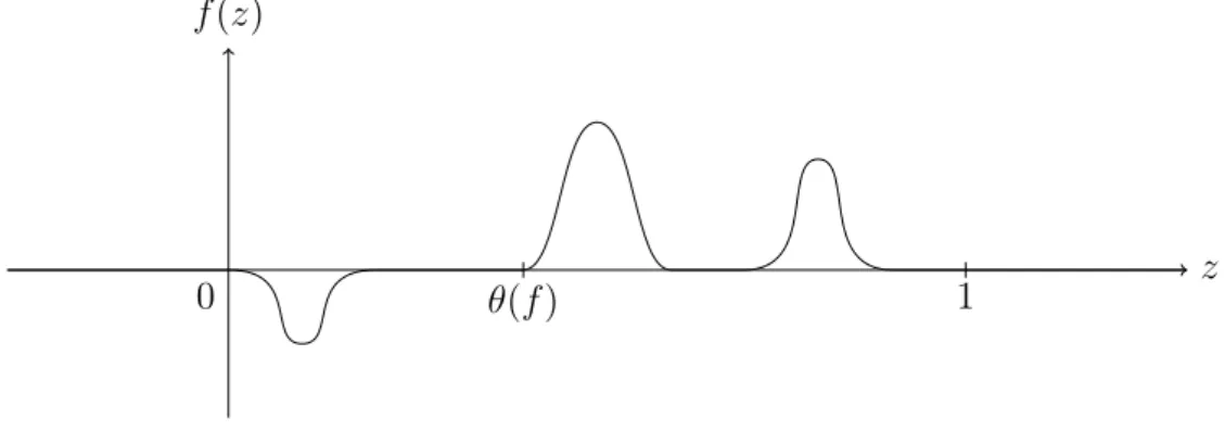
Definition 2.6 (Nonlinearity of basic type) A function f ∈ C

( R

× R , R ) is called a nonlinearity of basic type, if:

(i) f (x, z) = 0 for all z 6∈ (0, 1), x ∈ R

(ii) f (·, z) is 1-periodic in every component of x for every z ∈ [0, 1].

(iii) There is θ ∈ (0, 1) such that f (·, z) ≤ 0 for z ≤ θ and f(·, z) ≥ 0 for z ≥ θ.

We define

θ(f) := sup{θ ∈ (0, 1) : f (·, z) ≤ 0 for z ≤ θ and f (·, z) ≥ 0 for z ≥ θ} ∈ (0, 1].

1 z

f (z)

0 θ(f )

Figure 2.1.: An x-independent nonlinearity of basic type.

We will introduce several properties that nonlinearities of basic types can additionally have. Some of them refer to the (ε, b)-problem.

Definition 2.7 (Properties of nonlinearities) Let f be a nonlinearity of basic type.

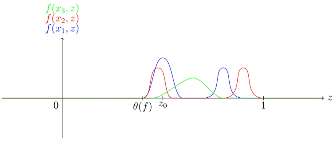
Covering Property. We say that f has the covering property, if (1) θ(f) ∈ (0, 1),

(2) for every z ∈ (θ(f), 1), there is x ∈ T

, such that f (x, z) > 0.

Strong Covering Property. We say that f has the strong covering property if f has the covering property and there exists z

∈ (θ(f ), 1) with f(x, z

) > 0 for all x ∈ T

.

Negative Wavespeed Property. We say f has the negative wavespeed property (with respect to the matrix field (a

)

and the unit vector k), if there exist constants b

> 0, ε

> 0 and c

< 0, such that for b ≥ b

, 0 < ε ≤ ε

, every solution (U

, c

) of (2.7), (2.8) satisfies c ≤ c

.

Combustion Type. We say that f is of combustion type, if f ≥ 0.

In all the existence results, f is supposed to have the covering property. Nevertheless, it will be important to consider the (ε, b)-problem for nonlinearities without this property.

The reason is that the (ε, b)-solutions in case of the nonlinearities without covering property are needed as comparison solutions. With these comparison solutions, we can then estimate the wavespeed in the case of nonlinearities with the strong covering property.

θ(f ) 1 z

f (x

, z) f (x

, z) f (x

, z)

0 z

Figure 2.2.: A nonlinearity of combustion type with the strong covering property.

2.2. Main results

Our first result is an existence result under an abstract assumption on f .

Theorem 2.8 (An abstract existence result) Let (a

)

be a matrix field and k be a unit vector as in the general assumptions. Furthermore, let f be a nonlinearity of combustion type with f |

∈ C

(T

× [0, 1]), which has the covering property and the negative wavespeed property (with respect to the matrix field and the vector k). Then there is a traveling wave solution (u, c) of type I as defined in definition 2.1 with c < 0.

Moreover, the strict inequalities 0 < u < 1 and u

> 0 hold. Additionally, the regularity u

∈ W

( R

) holds for any 2 ≤ p < ∞.

As a corollary, we will get the following result. We conclude it by showing that nonlinearities of combustion type with the strong covering property have the negative wavespeed property.

Theorem 2.9 (Existence of traveling wave solutions of type I) Let (a

)

be a matrix field and k be a unit vector as in the general assumptions. Furthermore, let f be a nonlinearity of combustion type with f|

∈ C

(T

×[0, 1]), which has the strong covering property. Then there is a traveling wave solution (u, c) of type I as defined in definition 2.1 with c < 0. Moreover, the strict inequalities 0 < u < 1 and u

> 0 hold.

Additionally, we have u

∈ W

( R

) for any 2 ≤ p < ∞.

Under additional regularity assumptions on f , we can prove that the solution of type I has enough regularity to be transformed into a solution of type II. See remark 2.20.

Theorem 2.10 (Existence of traveling wave solutions of type II) Let (a

)

be a matrix field and k be a unit vector as in the general assumptions. Furthermore, let f be a nonlinearity of combustion type with f |

∈ C

(T

× [0, 1]), which has the negative wavespeed property (for example because it has the strong covering property).

If moreover f

∈ C

(T

× [0, 1]) for some α

∈ (0, 1), then there is a traveling wave solution (U, c) of type II as defined in 2.2 with c < 0. Moreover, the strict inequalities 0 < U < 1 and U

> 0 hold.

Theorems 2.8, 2.9 and 2.10 should be compared to theorem 0.1 of [21]. For the compar- ison, see the comments in remark 2.20 below.

For the monotonicity and uniqueness results, we require less regularity for the matrix field than in the general assumptions:

Theorem 2.11 (Monotonicity) Let (a

)

be a C

(T

)-matrix field, which is sym- metric and uniformly elliptic. Furthermore, let f be a nonlinearity of combustion type with f|

∈ C

(T

× [0, 1]). Suppose that there is ε > 0 such that

f

(x, z) ≤ 0 for all (x, z) ∈ T

× [1 − ε, 1].

Let (u, c) with c < 0 be a traveling wave solution of (2.3), (2.4) as in definition 2.1.

Then u is increasing in t and the strict inequalities 0 < u < 1 and u

> 0 hold.

Theorem 2.12 (Uniqueness) Let (a

)

and f be as in theorem 2.11. Furthermore let (u, c) and (u

, c

) with c, c

< 0 be two traveling wave solutions of (2.3), (2.4) as in definition 2.1. Then c = c

and there is some t

∈ R such that u(t + t

, x) = u

(t, x) for all (t, x) ∈ R × R

.

Theorems 2.11 and 2.12 should be compared to theorems 0.2 and 0.3 of [21]. For com- ments, see remark 2.23.

2.3. A critical discussion of the results of Xin

In this section we will describe the work of Xin [21]. Xin considers the reaction-diffusion equation in nondivergence form:

u

=

n

X

i,j=1

a

(x)u

+ g(u) on R

. (2.9)

He assumes that (a

(x))

is a positive definite matrix, smooth and 1-periodic in each

component. Moreover, g is a combustion nonlinearity. By his definition, that means

g ∈ C

([0, 1], R ) with g ≡ 0 in [0, θ] for some θ = θ(g) ∈ (0, 1) and g > 0 in (θ, 1), as

well as g(1) = 0. For a given unit vector k and an unknown constant c, Xin is looking for a solution of the form U (s, y) = U (k · x − ct, x), which satisfies U (−∞, y) = 0, U(+∞, y) = 1 and U (s, ·) is 1-periodic in every component of y. In (s, y)-coordinates, the equation for U becomes

n

X

i,j=1

a

(y)(k

∂

+ ∂

)(k

∂

+ ∂

)U + cU

+ g(U ) = 0 on R

, (2.10)

0 ≤ U ≤ 1, U (−∞, y) = 0, U(+∞, y) = 1, U (s, ·) 1-periodic. (2.11)

2.3.1. Xin’s main results

The main results of Xin can be collected in the following three theorems:

Theorem 2.13 (Existence) The problem (2.10), (2.11) with a combustion nonlinear- ity g has a classical solution (U, c), which additionally satisfies

0 < U < 1 for all (s, y) ∈ R × T

U

(s, y) > 0 for all (s, y) ∈ R × T

c < 0.

Theorem 2.14 (Monotonicity) If the combustion nonlinearity g satisfies g

(1) < 0 and (U, c) is a classical solution of the problem (2.10), (2.11), then U

(s, y) > 0 for all (s, y) ∈ R × T

.

Theorem 2.15 (Uniqueness) If the combustion nonlinearity g satisfies g

(1) < 0 and (U, c), (U

, c

) are two classical solutions of the problem (2.10), (2.11), then c = c

and there is s

∈ R , such that U (s, y) = U

(s + s

, y) for all (s, y) ∈ R × T

.

2.3.2. Xin’s proof of existence

In order to prove theorem 2.13, Xin begins with an elliptic regularization. Consider the weight factor

r(y) :=

n

X

i,j=1

a

(y)k

k

(2.12)

and the linear elliptic operator L

U := εr(y)U

+

n

X

i,j=1

a

(y)(k

∂

+ ∂

)(k

∂

+ ∂

)U.

Then the elliptic regularization problem for (U, c) (we like to call it the (ε, b)-problem) is the following problem:

L

U + cU

+ g(U ) = 0 on (−b, b) × R

, (2.13)