C. Berndt1 , W.‐C. Chi2 , M. Jegen1, E. Lebas1,3 , G. Crutchley4 , S. Muff1, S. Hölz1 , M. Sommer1, S. Lin5, C.‐S. Liu6 , A. T. Lin7, D. Klaeschen1 , I. Klaucke1, L. Chen2,6,8, H.‐H. Hsu5,6 , P. Kunath1,5, J. Elger1, K. D. McIntosh9, and T. Feseker10
1GEOMAR Helmholtz Centre for Ocean Research Kiel, Kiel, Germany,2Institute of Earth Sciences, Academia Sinica, Taipei, Taiwan,3Now at Institute for Geosciences, Christian‐Albrechts‐University of Kiel, Kiel, Germany,4GNS Science, Lower Hutt, New Zealand,5Institute of Oceanography, National Taiwan University, Taipei, Taiwan,6Ocean Center, National Taiwan University, Taipei, Taiwan,7Department of Earth Sciences, National Central University, Zhong‐li, Taiwan,8Now at GEOMAR Helmholtz Centre for Ocean Research Kiel, Kiel, Germany,9Institute for Geophysics, University of Texas at Austin, Austin, TX, USA,10GEOFACT, Bonn, Germany
Abstract
The northern part of the South China Sea is characterized by widespread occurrence of bottom simulating reflectors indicating the presence of marine gas hydrate. Because the area covers both a tectonically inactive passive margin and the termination of a subduction zone, the influence of tectonism on the dynamics of gas hydrate systems can be studied in this region. Geophysical data show that there are multiple thrust faults on the active margin while much fewer and smaller faults exist in the passive margin.This tectonic difference matches with a difference in the geophysical characteristics of the gas hydrate systems. High hydrate saturation derived from ocean bottom seismometer data and controlled source electromagnetic data and conspicuous high‐amplitude reflections in P‐Cable 3‐D seismic data above the bottom simulating reflector are found in the anticlinal ridges of the active margin. In contrast, all geophysical evidence for the passive margin points to normal to low hydrate saturations. Geochemical analyses of gas samples collected at seep sites on the active margin show methane with heavyδ13C isotope composition, while gas collected at the passive margin shows light carbon isotope composition. Thus, we interpret the passive margin as a typical gas hydrate province fueled by biogenic production of methane and the active margin gas hydrate system as a system that is fueled not only by biogenic gas production but also by additional advection of thermogenic methane from the subduction system.
Plain Language Summary
Gas hydrates are ice‐like crystals in marine sediments. They store an enormous amount of carbon and may be used as a future energy source. So far, little is known about the geological processes that control the distribution of gas hydrates. In this study we have combined a very wide range of geophysical and geochemical data tofind out if the movements in the Earth crusts matter for the amount of gas hydrate in the surface rocks. We found out that there is much more hydrate in areas where there is a lot of movement than in those that are stable. This contradicts the previously held believes. It seems a good idea to focus hydrate exploration close to subduction zones rather than on old continental margins.1. Introduction
Gas hydrates are ice‐like compounds of water and gas that are stable at high pressure and low temperatures, for example, in continental margin sediments or within permafrost regions. Because gas hydrates in marine sediments contain at least as much carbon (500–4500 Gt; Buffett & Archer, 2004; Piñero et al., 2013;
Wallmann et al., 2012) as is present in the entire atmosphere (~720 Gt; Falkowski et al., 2000), it is important to understand their distribution and the geological processes that control their formation and dissociation. As most of the carbon that is stored within gas hydrates is present in the form of methane, several countries have begun extensive research programs to investigate whether gas hydrates can be used as a future energy source (Johnson & Max, 2006). There are, however, also other reasons to study marine gas hydrates: they may play a role in submarine slope stability (Sultan et al., 2004), they may be linked to climate change (Berndt, 2013;
Dickens, 2011), and to some extent they control the functioning of benthic ecosystems (Sibuet & Roy, 2003).
Determining the distribution and saturation of gas hydrate is essential for assessing the commercial viability of exploiting gas hydrates as a future energy source and also for understanding the role of gas hydrates in
©2019. American Geophysical Union.
All Rights Reserved.
Key Points:
• Gas hydrate formation depends on tectonically controlled advection of gas
• Offshore SW Taiwan gas hydrate saturations are higher in the active margin than in the passive margin
• Data evaluation combines seismic and controlled source electromagnetic data
Correspondence to:
C. Berndt, cberndt@geomar.de
Citation:
Berndt, C., Chi, W.‐C., Jegen, M., Lebas, E., Crutchley, G., Muff, S., et al. (2019).
Tectonic controls on gas hydrate distribution off SW Taiwan.Journal of Geophysical Research: Solid Earth,124, 1164–1184. https://doi.org/10.1029/
2018JB016213
Received 12 JUN 2018 Accepted 7 JAN 2019
Accepted article online 12 JAN 2019 Published online 8 FEB 2019
climate change, slope stability, and ecosystem functioning. In spite of 30 years of research, little is known about the distribution of marine gas hydrate. It is reasonable to assume that most gas hydrate is found directly above the base of the hydrate stability zone (BHSZ) because gas rising from below may form hydrate as soon as it enters the hydrate stability zone (Boswell et al., 2012; Pecher et al., 2001). However, drilling off Vancouver Island and in the South China Sea has shown that high hydrate saturations may also be encoun- tered much higher up into the hydrate stability zone (Malinverno et al., 2008; Sha et al., 2015) and the few dedicated attempts to quantify gas hydrates by deep sea drilling are not conclusive about the distribution and saturation variations of gas hydrate in continental margin systems. Therefore, numerous studies have tried to assess hydrate saturations through the use of geophysical methods. These range from simple mapping of the bottom simulating reflector (BSR), which can provide information on the minimum extent of a gas hydrate province (Bünz et al., 2003), to full waveform inversion of multichannel seismic reflection (MCS) data (Delescluse et al., 2011), and to the use of converted wave information provided by ocean bottom seism- ometers (OBSs) and ocean bottom cables (Bünz, 2004; Bünz et al., 2005; Mienert et al., 2005; Schnurle et al., 2005). Also, controlled source electromagnetic (CSEM) measurements have been used for deriving 2‐D mod- els of hydrate saturation (Constable et al., 2016; Schwalenberg et al., 2010; Weitemeyer et al., 2006).
While most of these methods alone have not been able to identify a strong link between geological structures and variations in gas hydrate saturation, there are several noteworthy exceptions. Tomographic inversion of three‐dimensional OBS data from mid‐Norway show significantly increasedPwave velocities at the location of pipe structures in seismic reflection data. This observation suggests that focusedfluid migration may lead to particularly high hydrate saturation where gas‐richfluids enter the gas hydrate stability zone (Plaza‐ Faverola et al., 2010). This is consistent with drilling‐derived hydrate saturations that show particularly high hydrate saturations wherefluidflow is focused by permeable structures or lithologically controlled perme- ability variations (Collett et al., 2012; Tréhu et al., 2004). The Hikurangi Margin off New Zealand provides another example for focusedfluid migration generating high saturation gas hydrate deposits at the base of the hydrate stability zone (Crutchley et al., 2015). In this case the lateral changes in hydrate saturation were derived from detailed velocity analysis of seismic reflection data. These observations are consistent with the notion of focused gas hydrate systems (Milkov & Sassen, 2002).
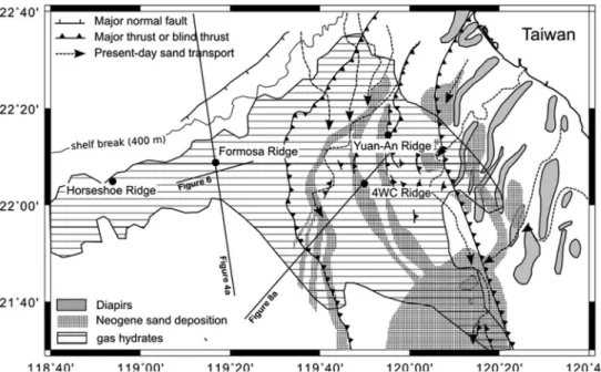
Here, we present new seismic, electromagnetic, and seafloor mapping data to analyze the influence of tec- tonic processes on the distribution of natural gas hydrate. To this end we will investigate (a) if there are sys- tematic differences in the gas hydrate distribution and saturation between the passive and active margin SW off Taiwan and (b) to what extent tectonic and lithological controls can explain such differences (Figure 1).
2. Geological Setting
The northern part of the South China Sea consists of a passive margin stretching from the island of Taiwan in a southwesterly direction (Figure 2). IODP expedition 349 showed that seafloor spreading started around 33 Ma varying by 1–2 Ma along the northern continent‐ocean boundary and that there was a ridge jump at 23.6 Ma (Li et al., 2014). Using 6‐km‐long offset seismic reflection data, McIntosh et al. (2013) propose that the northern part of the South China Sea consists of thinned continental crust, with a layer of magmatic underplating. More detailed analyses of high‐quality data sets suggest that there is hyperextended continen- tal crust along the northern margin of the South China Sea plate near Taiwan (McIntosh et al., 2013).
Magnetic data have been interpreted to show at least one ridge jump during the spreading, and that spread- ing ended at about 15.5 Ma (Barckhausen & Roeser, 2004; Briais et al., 1993), which is consistent with the IODP drilling results that put the end of spreading at ~15 Ma in the East Subbasin and ~16 Ma in the Southwest Subbasin (Li et al., 2014).
South of Taiwan the lithosphere of the Eurasian plate is subducting eastward beneath the Philippine Sea plate with a high rate of 7 to 9 cm/year (Yu et al., 1997). The initial collision zone is probably near latitude 20°N where a proposed continent‐ocean boundary enters the trench. To the north the subduction changes into arc‐continent collision. This results in a wide range offluid and gas migration systems that form cold seeps at the surface. Hence, there are both active and passive margins in this small offshore region, where a widespread BSR has been mapped (Liu et al., 2006). The presence of gas hydrates in the subsurface was supported both by geophysical methods (Schnurle et al., 2005) and through logging while drilling measure- ments (Wang et al., 2017). Gas hydrates have also been sampled and measured by in situ Raman
spectroscopy in the surface sediments (Zhang et al., 2017). Two decades of geochemical studies have revealed that both biogenic and thermogenic methane is discharged from the seafloor off SW Taiwan (Chen et al., 2017). Theflow hasflux rates of 2.71 × 10⁻³to 2.78 × 10⁻¹and 1.88 × 10⁻¹to 3.97 mmol·m
−2·day−1at the sulfate methane interface and at the sediment seawater surface, respectively. Gravity corer sediment samples from the top 6 m of sediments do not show thermogenic gas signatures for the passive margin where d13C ratios are between−90‰and−68‰VPDB and C1/C2+ratios are between 900 and 2,000. Opposed to this the d13C ratios and C1/C2+ratios show admixing of thermogenic gas starting from the deformation from eastward (Chen et al., 2017). There are, however, also a number of sites on the active margin that only show biogenic gas seepage. The site with the most pronounced thermogenic gas affinity is Tsanyao Mud Volcano on the upper slope of the active margin which has more than 10% high‐order (>C2) hydrocarbons (Chen et al., 2017). Given that the SW Taiwanese margin is generally characterized by a geothermal gradient between 42 and 75 mK/m (Berndt, 2013) the top of the present day oil window should be at a depth of 1,600 to 2,800 m below seafloor and the base between 2,200 and 3,800 m below seafloor.
Due to a lack of drilling information the lithostratigraphy off SW Taiwan is poorly defined. On top of the rifted Mesozoic basement a 1‐to 2‐km‐thick Miocene succession on the shelf of the Formosa Straits thins quickly into the South China Sea. It is overlain by up to 3‐km‐thick Plio‐Pleistocene clastic sediments (Lin et al., 2008). Taiwan has some of the highest denudation rates in the world and large amounts of clastic sedi- ments are transported through the major canyons into the South China Sea (Lin et al., 2013). The clastic sedi- ments are predominantly confined to the canyons and the deep sea fans, whereas the distal parts are dominated by hemipelagic sedimentation. Canyon incision in the northern margin of the South China Figure 1.Bathymetric map of the study area, which is located at the northern termination of the Manila Trench where the Luzon Arc collides with the continental margin of Eurasia. The subducted Eurasian plate is continental at least north of 20°30′N (Eakin et al., 2014), whereas the Luzon Arc consists of oceanic island arc crust.
Sea reworked the top of the Plio‐Pleistocene sequences as did contour currents that led to a buildup of sedi- ment drifts at the foot of the slope.
3. Methods
3.1. Multi‐Channel Seismic Acquisition and Processing
The MCS reflection data were acquired using R/V Marcus Langseth. The sources consisted of four strings, each with 9 Bolt airguns, with a total volume of ~6,600 in3, which was towed at 8‐m depth andfired at a shot spacing of 50 m. The data (Figures 3–8) were collected with a 6‐km streamer towed at 9‐m depth, with a recording length of 15 s. The resulting data were binned at 6.25 m. Close to the seafloor horizontal and ver- tical resolution is approximately 6.25 and 15 m, respectively. Penetration is up to 20 km. Processing included a standard predictive gapped deconvolution for sharpening the wavelet. Afterward a 2‐D surface‐related multiple elimination and Radonfiltering was applied to suppress the seafloor multiples. Residual multiples were further suppressed using inside mute and time variant frequencyfilters. The data shown in Figures 4, 6, and 8 were then prestack time migrated using Kirchhoff migration. For more details on the MCS processing see Lester and McIntosh (2012).
To determine the seismic velocities for Four‐Way Closure Ridge, we carried out afirst‐pass Kirchhoff pre- stack time migration using a starting migration velocity model. We then used a linear and parabolic curve scanning routine for automatic reflection picking from the common image point gathers. These reflection picks were used for a 2‐D travel time inversion to refine the starting velocity model. We iteratively improved the velocity model with successive prestack time migration, automatic reflection picking, and travel time inversions. We then carried out Kirchhoff depth migration, automatic reflection picking, and ray tracing and tomography. As in the time domain, iterative improvements in the velocity model were made with suc- cessive depth migrations and tomographic inversions. Derivation of the seismic velocity model for the MCS line crossing Formosa Ridge (Figure 5b) is described in Hsu et al. (2017) and is based on prestack depth migration focusing analysis. Sensitivity analysis suggests that the velocities are accurate within ±8% for anomalies of more than 100 m lateral and 20 m vertical extent down to BSR depth but that the shape of the velocity anomalies is affected by subjective picking choices of the interpreter.
Figure 2.Geological map of the study area SW off Taiwan. The westernmost thrust fault marks the deformation front.
Thus, the study site of Formosa ridge is located on the passive margin, while Yuan‐An Ridge and Four‐way Closure (4WC) Ridge represent typical settings for the active margin. Tectonic structures from (Lin et al., 2009; Schnurle et al., 2005; Sibuet & Hsu, 2004). Distribution of sand and sand transport from (Lin et al., 2013).
3.2. P‐Cable High‐Resolution 3‐D Seismic Imaging
Three 3‐D seismic cubes (Formosa Ridge, Four‐Way Closure Ridge, and Yuan‐An Ridge) were collected with the multichannel 3‐D seismic P‐
Cable system (Planke et al., 2009) during the cruises SO227, OR5‐1306‐
1, and OR5‐1415 on board the vessels R/V Sonne (Berndt, 2013) and R/V Ocean Researcher 5, respectively. The system consists of a number of parallel streamers that are attached to a cross cable, which is dragged perpendicular to the vessels navigation direction. The source for each sur- vey area was a 210‐in3GI gun,fired every 4 s generating a seismic signal with a dominant frequency of 110 Hz and a usable bandwidth from 50 to 350 Hz. The shot intervals resulted in an average shot spacing of 6– 9 m (average ship speed of 3–4 knots). The data were sampled at 1 ms.
Processing included navigation quality control, geometry corrections, trace editing, static time corrections, and band‐passfiltering (with low‐ cut frequency 50 Hz). Noise bursts in the data volumes were replaced by average spectral amplitudes from the two non‐zero neighboring traces in overlapping time–space windows. F‐K domain spatial predictionfilters were used to suppress random noise, coherent noise and swell noise simultaneously. Remaining anomalous amplitudes were detected and rejected in a sliding window. Normal move‐out corrections with an aver- age velocity of the water column and constant gain were applied before stacking. All four cubes were stacked in 3.125 × 3.125‐m bins. Trace inter- polation was performed in the in‐line and cross‐line direction and a post- stack 3‐D F‐K coherency filter was integrated into the processing workflow. As the geology of the survey areas implies strong lateral changes in seismic velocity we tested various migrations. First, we applied a Stolt migration with a constant velocity of 1,500 m/s. This was then fol- lowed by a residual FD time migration using a smoothed velocityfield derived from the OBS data, which was used for thefinal processing result.
Thefinal cubes have a maximum resolution of 3.125 × 3.125 × 7.5 m at the seafloor.
3.3. OBS Deployments
The OBS data reported in this study were collected in 2013 during the TAIFLUX cruise aboard the R/V Sonne. Each instrument was equipped with a hydrophone and a three‐component geophone. We deployed them along two dip transects, consisting of 12 stations each above Formosa Ridge (Figure 3) and Four‐Way Closure Ridge (Figure 7). The transect for Formosa Ridge was oriented in a NW‐SE direction along the ridge, while the transect above Four‐Way Closure Ridge was oriented in WSW‐ENE direction over the northern part of the ridge. The OBS spacing at Formosa Ridge was generally between 460 and 560 m, but up to
>1 km in places in order to cover the entire ridge. At Four‐Way Closure Ridge, the instruments were placed 600 to 800 m apart. Only one station was deployed 920 m away from the previous one. The seismic source was the same as during the P‐Cable acquisition (210‐in3 GI gun) and the shot firing rate was 5 s.
Sampling rates of 500 and 1,000 Hz were used by the instruments at Formosa and Four‐Way Closure ridges, respectively. The instruments were relocated using the direct wave arrivals. First arrivals recorded by each station can be clearly seen along the entire profiles in each survey. Preprocessing of the data consisted of the logger's internal clock‐drift corrections (specific to each instrument), shot‐time delay (30 ms), and recor- der delay (25 to 44 ms depending on the sampling rate used) in order to adjust the clock of each OBS station to the GPS base time. No gain correction was applied to the data to preserve relative amplitudes. Picking of thefirst and secondary arrivals was performed manually on the hydrophone data using the PASTEUP soft- ware (Fujii et al., 2015). Nofiltering was applied to the data while picking thefirst arrivals, but a frequency band‐passfiltering of 30‐60‐300‐400 Hz was assigned to the data while picking the secondary arrivals in order to enhance certain phases. The data were retrieved from all instruments with good quality, except at Formosa Ridge where records from two OBS stations (002/006) could not be extracted and OBS 011, which did not function properly in both areas. The steepflanks of Formosa Ridge reduce the accuracy of OBS Figure 3.Bathymetric map of Formosa ridge showing canyon incision and
the configuration of the geophysical experiments. The locations of multi- channel seismic reflection profiles in Figures 4b and 6 are indicated in black (for the entire length of Figure 6, see Figure 2). The white line indicates the extent of the joint P‐Cable‐OBS‐CSEM interpretation in Figures 5a and 5c.
OBS = ocean bottom seismometer; CSEM = controlled source electromagnetic.
relocation and result in side reflections in some of the OBS data. As a consequence, only three out of 12 OBS could reliably be used at Formosa Ridge. We derived aPwave velocity model in each area using ray tracing forward modeling in the RAYINVR software, which follows a top‐down approach (Zelt & Smith, 1992). The models are composed of 7 and 13 layers at Formosa and Four‐Way Closure Ridges, respectively. The apparent seismic velocities derived for each phase were carefully chosen manually, until the smallest RMS and χ2 values were obtained. Table 1 summarizes the number of picks per phase and associated RMS andχ2 values, for the two models. Prominent reflections correlating well between the OBS and P‐
Cable data were used as model interfaces. The high‐resolution of the P‐Cable data (3.125 m horizontal,
~7.5 m vertical) provided good constraints on the geometry of the interfaces, which helped to improve the models by reducing uncertainties related to the geometry. However, the ray tracing method is not sensitive to small (100 by 100 m)‐scale velocity anomalies and the resulting velocities have to be considered average velocities on a scale larger than this. By varying the interval velocities in the different layers and comparing the calculated arrival times to the observed arrival times for the reflections at the base of the gas hydrate stability zone we constrain the sensitivity of this method. Whereas the sensitivity is good (±50 m/s) for the long, continuous reflections within the top 300 ms below the seafloor, the complex structure and the limited observation offsets of the arrivals close to the BSR imply errors of up to
±150 m/s for the interval just above the BSR.
3.4. CSEM Surveying
Marine CSEM measurements were carried out with ocean bottom electromagnetic (OBEM) receivers, which measure two horizontal components of the electric field using 11.2‐m‐long pairs of electrode arms.
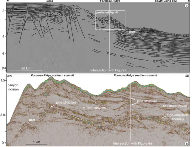
Figure 4.Seismic images of Formosa Ridge (see Figures 2 and 3 for locations). (a) Time migrated 6‐km‐offset multichannel seismic reflection data showing normal faulting under the shelf break and sediment waves on the continental slope that are indicative of contourite deposits. (b) Arbitrary line extracted along the crest of Formosa Ridge from high‐resolution 3‐D seismic data.
Generally, the system is operated at high‐frequency (10 kHz,Efields only) for CSEM measurements but also allows for low‐frequency (10 Hz) magnetotelluric (MT) measurements, in which the magnetic field components are also measured via a fluxgate. A switch between these CSEM and MT modes can be performed via acoustic signal or via a predetermined timetable. Further details of the receiver and transmitter systems can be found in Hölz et al. (2015).
For our CSEM source we used GEOMAR's newly developed Sputnik system, a frame based transmitter deployment system. The system consists of a transmitter frame, which is lowered and placed onto the sea- floor using the ship's winch cable. When placed stationary onto the seafloor it unfolds two pairs of electrode arms, which allow for the transmission of signals along two perpendicular polarizations with 10‐m‐long dipoles. Afterfinishing measurements at one site, the system is lifted up to a safe distance from the Figure 5.Collocated OBS‐derivedPwave velocities (a) and CSEM‐derived apparent electrical resistivities (c) overlain on high‐resolution 3‐D seismic data for the southern part of Formosa Ridge (coverage shown in Figure 3). Panel (b) shows the pre‐stack depth migration velocities overlain over the prestack depth migrated multichannel seismic reflection line that strikes at an angle to the OBS and CSEM data (after Hsu et al., 2017). Except for the apparent electrical resistivity anomaly close to a pipe structure, the seismic velocities and apparent electrical resistivities show normal ranges for passive margins. White dots in panel (c) show midpoints for source receiver pairs at depth corresponding to offset where apparent resistivity has been determined and interpolated. OBS = ocean bottom seismometer; CSEM = controlled source electromagnetic; BSR = bottom simulating reflector.
seafloor (20–50 m) and is then moved to the next site. The transmitter, an enhanced version of the one described in Hölz et al. (2015), was operated with a maximum current of 48.9A at a 50% duty cycle.
Transmissions at each site usually lasted about 3–4 min.
CSEM measurements in thefirst work area were carried out along the Formosa Ridge, where 12 OBEM receivers werefirst deployed by cable to the seafloor along a 7.5‐km‐long profile (Figure 3). The Sputnik deployment system was then used to position the transmitter at a total of 46 locations along the profile.
Due to acoustic problems, the activation of the high‐frequency CSEM mode only worked for six of the OBEM receivers, while the other six remained in the low‐frequency MT mode and, thus, did not yield any valuable data for the CSEM experiment.
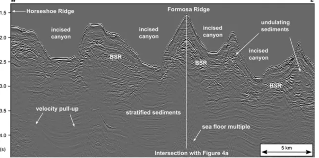
In the second work area the 12 OBEM receivers were placed along a 4.8‐km‐long profile across the Four‐Way Closure Ridge (Figure 2). The activation procedure of receivers was adjusted to include timetables and after Figure 6.Multichannel seismic reflection data line MGL0905‐8r showing similar seismic character of the ridges along the passive margin. See Figure 3 for location.
BSR = bottom simulating reflector.
Figure 7.Overview map for the active margin showing the configuration of the geophysical experiments at Four‐Way Closure Ridge. The white line indicates the extent of the joint P‐Cable‐OBS‐CSEM interpretation in Figure 9.
OBS = ocean bottom seismometer; CSEM = controlled source electromagnetic.
that 11 of the 12 receivers worked as expected. The Sputnik deployment system was used to position the transmitter at a total of 44 locations along the profile, resulting in a much denser data set compared to the Formosa Ridge working area.
In both working areas processing yielded transients above the noisefloor for transmitter‐receiver separa- tions up to a maximum of 1,200 m. At most sites useful data with signal‐to‐noise ratios above 10 (at the DC level) were acquired to distances up to 800 m. The use of two transmitter polarizations is quite Figure 8.Reflection seismic images of the active margin. (a) Long‐offset multichannel seismic reflection line MGL0905‐10 showing the anticlinal ridges from the deformation front eastward. Thrust faults are clearly imaged below the frontal ridge and are less clear toward the east. Interpretation of the thrust underneath Four‐ Way Closure Ridge is based on the configuration of sedimentary horizons above. (b) High‐resolution 3‐D seismic inline 1309 showing the anomalous high‐ amplitude reflections above the BSR. Note: The BSR, although not clearly imaged everywhere, can be confidently picked regionally from full 3‐D interpretation of the data volume. (c) Three‐dimensional view to the southeast illustrating the spatial relationship between the BSR, the high‐amplitude reflections above the BSR, and the seep sites. BSR = bottom simulating reflector.
uncommon for marine CSEM measurements, but can be handled by the concept of rotational invariants (Hölz et al., 2015), which was used by Swidinsky et al. (2015) to derive a rapid imaging scheme for two polarization measurements in terms of apparent resistivities. This imaging has to be considered as afirst‐ pass interpretation, which can only provide a general idea about the true resistivities. Also, the apparent resistivity sections derived from the CSEM data only reveal large‐scale (>200 m) features, whereas smaller scale anomalies in the resistivity structure cannot be determined by this approach.
3.5. Multibeam Echo Sounding
Bathymetric data have been acquired using a Simrad EM120 system providing 191 simultaneous beams with 2° × 2° beam opening angle. During RVSonnecruise SO227 the system was used in equidistant mode. The total swath width was 120° and survey speed was generally 8 knots during dedicated bathymetric survey lines, while bathymetric data recorded during sidescan sonar and P‐Cable surveys were acquired using 90° total swath width and 3.0 knots survey speed. A track spacing of 1,300 m for the side scan sonar and 60 m for the P‐cable surveys resulted in high sounding density. This allowed to grid the manually cleaned bathymetric data at Formosa and Four‐Way Closure Ridge at 10‐and 25‐m grid spacing, respectively. The regional survey has been gridded at 50‐m spacing.
4. Results
4.1. Passive Margin
The shelf between the Chinese mainland and Taiwan is up to 200‐m deep. MCS data (Figure 4) show numer- ous normal faults that are presumably related to Cretaceous to Oligocene rifting and reach partly up to the seafloor. Below the shelf break, down to approximately 2,000‐m water depth, canyons with steep flanks incise several hundred meters deep into the slope sediments. MCS data show a distinct change from tilted fault blocks that are observed landward of the shelf break to a slope facies with seafloor parallel bedding sea- ward of the shelf break. This facies is at least 3‐s two‐way travel time (TWT) thick. In the top 300‐to 600‐ms TWT, sedimentary reflectors are truncated by erosional unconformities in the upper part of the slope and undulating reflectors with highly variable separation in the lower part. Both the underlying slope facies and the more chaotic upper sediments do not show signs of tectonic faulting.
4.1.1. Formosa Ridge
Formosa Ridge is one of the ridges on the northern slope of the South China Sea that is formed by canyon incision into the upper chaotic seismic facies (Figures 4 and 6). The P‐Cable 3‐D seismic data show that the undulating sedimentary features on the lower slope are sediment waves and that the truncations of
Table 1
Picking Parameters and Model Fitting for 11 Phases of OBS Data Used to Establish the Two Velocity Models for Formosa Ridge and Four‐Way Closure Ridge
Formosa ridge Four‐way closure ridge
Number of data points used 3,072 Number of data points used 12,014
RMS travel time residual (s) 0.006 RMS travel time residual (s) 0.004
Normalizedχ2 0.093 Normalizedχ2 0.058
Phase ID # picks trms(s) χ2 Phase ID # picks trms(s) χ2
1 1,526 0.007 0.107 1 7,998 0.004 0.074
2 383 0.006 0.078 2 960 0.003 0.035
3 503 0.005 0.051 3 559 0.002 0.017
4 574 0.002 0.016
5 405 0.002 0.024
6 41 0.002 0.027
7 516 0.003 0.032
8 180 0.003 0.040
9 178 0.002 0.015
10 310 0.003 0.035
11 293 0.003 0.037
Note. OBS = ocean bottom seismometer.
the reflectors in the northern part of Formosa Ridge are caused by formerly incised and now refilled canyons (Figure 4b). The MCS data show that the sediments related to these facies cover horizontally stratified sedi- ments underneath the crest of ridge.
A prominent BSR with reverse seismic polarity crosscuts the sedimentary reflectors within Formosa Ridge (Figure 4b). The MCS data clearly show its reversed polarity with respect to the seafloor. The BSR is located between 0.5‐s TWT beneath the crest of the ridge and 0.23‐s TWT underneath the canyons.
Both the P‐Cable and MCS data show increased seismic amplitudes right below the BSR, but high ampli- tudes are generally absent above the BSR (Figure 4b). Exceptions are found in the vicinity of a vertical seismic anomaly underneath the southern summit of Formosa Ridge, at the base of some of the major incised and refilled canyons, within the upper limbs of some of the undulating seismic reflector packages and just above the BSR in an approximately 500‐ by 800‐m‐wide area underneath the southern part of Formosa Ridge.
The OBS‐derived seismic velocity rise from less than 1,600 m/s at the seafloor to 1,800 m/s about 300 ms TWT below the seafloor and up to 1,850 m/s directly above the BSR (Figure 5a). Because of the 2,000‐to 3,000‐m separation of the OBS and the resulting ray coverage, these values have to be considered average values on a 1‐km horizontal and 100‐m vertical scale. It is likely that there are small‐scale (10–100 m) high‐and low‐velocity anomalies in the three layers that are not visible at this resolution.
The seismic velocities derived from tomographic prestack time and depth migration velocity analysis of the MCS data from Formosa Ridge show a typical trend for hydrate provinces. The velocities increase from the seafloor to the BSR, which itself is characterized by a velocity inversion. The velocities just above the BSR range from 1,800 up to 2,100 m/s but such high velocities are confined to a 200‐m‐wide patch SSE of the southern summit of Formosa Ridge (Figure 5b). In the region NW of the summit where OBS01‐recorded arrivals both the OBS analysis and the pre‐stack depth migration velocity analysis yield velocities around 1,850 m/s. Below the BSR the velocities drop to 1,600–1,700 m/s within a layer that is about 100 to 200 m thick. Testing different velocities shows that there is a trade‐off between the thickness of the velocity anoma- lies and their absolute value, for example, the low‐velocity zone underneath the BSR may be thinner (80–120 m) if the interval velocities are as low as 1,450 m/s.
The apparent resistivity data derived from the CSEM receivers show a gradual increase in apparent electrical resistivity from less than 1Ωm at the seafloor to 2–3Ωm at the depth of the BSR (Figure 5c). A single anom- aly south of the southern summit of Formosa Ridge indicates an electrical resistivity higher than 4Ωm. This anomaly is located close to a pipe structure in the high‐resolution 3‐D seismic data. Similar to the OBS data, the sparseness of measurements means that we cannot rule out that there are small‐scale (100–300 m) anomalies with higher or lower electrical resistivity. Opposed to OBS data that are not sensitive to velocity anomalies at shallow depth except for those directly beneath the OBS location the electromagnetic data are most sensitive to shallow resistivity variations.
4.1.2. Regional Results for the Passive Margin
MCS data along the passive margin (Figure 6) show that Formosa Ridge is typical for all the ridges along the margin. The other ridges have similar seismic amplitude characteristics with a strong BSR and high‐ amplitude reflections below it. The internal structure of the ridges is also similar, with undulating seismic reflectors of variable thickness overlying horizontally stratified sediments. There is also no evidence for major faults under the other ridges.
4.2. Active Margin
Off SW Taiwan an accretionary prism extends up to 100 km westward from the Luzon Arc. While the prox- imal third of the prism is characterized by subsurface mud mobilization and anticline development above mud diapirs, the distal part of the accretionary prism out to the deformation front is characterized by thrust faults and blind thrusts that push up anticlines and monoclines that form N‐S oriented ridges. These are dis- sected by two major and several minor canyons. On high‐quality seismic lines some of the thrust faults are clearly imaged (Figure 8a) while they are not imaged beneath, some ridges, and generally on data with lesser quality. The décollement is generally imaged poorly on reflection seismic data and OBS‐derived velocity models (Eakin et al., 2014).
4.2.1. Four‐Way Closure Ridge
Based on side scan sonar data and preexisting 2‐D seismic data we selected Four‐Way Closure Ridge as a representative structure for the active margin (Klaucke et al., 2015). The crest of the ridge is at approximately 1,150‐m water depth, whereas the surrounding seafloor is between 1,500 and 1,700 m deep. West of the ridge is a slope basin while the western part of the ridge merges with another ridge that extends southward into the study area. The crest of this ridge is at 1,650‐m water depth and the slope basin west of this ridge is at 2,000‐m water depth. Neither the MCS data nor the P‐Cable data image clearly the thrust fault that must underlie Four‐Way Closure Ridge, although some high‐amplitude reflectors in the MCS data may be interpreted as fault plane reflections. The dip of sedimentary reflectors in Four‐Way Closure Ridge show it is an anticline, whereas the ridge west of it is a monocline with reflectors dipping uniformly to the west.
The P‐Cable seismic data show that a gas hydrate BSR exists beneath the easternflank of Four‐Way Closure Ridge and part of the westernflank as well as within the slope basin to the east (Figure 8b). It also underlies the adjacent ridge to the west, but it is absent or not well imaged between the two ridges, possibly because it dips in the same direction as strata in the western limb of the anticline. In the low‐frequency MCS data the BSR is characterized by reverse polarity with respect to the seafloor. The amplitude of the BSR reflection is highest underneath the ridge and slightly lower in the slope basin. Most strikingly, there are very high‐ amplitude reflections within Four‐Way Closure Ridge. These reflections occur in the lower half of the GHSZ, which is approximately 400 m thick (Figure 8b). An exception is a band of particularly high ampli- tudes that dips eastward although it is located in the western part of the anticline. Detailed mapping of this reflection band shows that it extends from about 160‐ms TWT below the surface in the core of the anticline toward the seabed on the westernflank where seafloor photography and side scan sonar imagery have shown large carbonate banks that are covered by dead bivalve beds (Klaucke et al., 2015).
In addition to the high‐amplitude reflections from within the core of the anticline, there is also an area where the amplitudes of the seismic reflections from slope basin sediments are significantly increased.
These acoustic anomalies occur where the BSR intersects the unconformity that forms the western boundary of the slope basin. The seismic character of these amplitude anomalies is very similar to the small areas of high‐amplitude reflections immediately above the BSR in Formosa Ridge.
The OBS‐derivedPwave velocities at Four‐Way Closure Ridge rise from 1,600 m/s at the seafloor to approxi- mately 1,700 m/s at BSR depth in the slope basin East of Four‐Way Closure Ridge (Figure 9a). Thus, they remain below the 1,850 m/s velocity derived for Formosa Ridge. However, in the area of the high‐amplitude reflections above the BSR in the core of the anticline that forms Four‐Way Closure Ridge,Pwave velocities must exceed 1,900 m/s tofit the data. There is a strong difference between the western area of high‐
amplitude anomalies where average velocities are approximately 1,900 m/s and the eastern part below the seep site wherePwave velocities rise up to 2,200 ± 150 m/s. Keeping the P‐Cable derived reflector geome- triesfixed, the bestfitting velocity for the lowermost part of the GHSZ is 2,350 m/s. The P‐Cable data show that the geology does not vary much along the ridge. Therefore, the two‐dimensional OBS transect should be a good representation of the ridge and the results of OBS modeling are more robust than the velocityfield derived for Formosa Ridge. Unfortunately, it is not possible to derive the velocity for the zone below the BSR except for a small area at the western termination of the slope basin where the velocity does not seem to decrease significantly (Figure 9a).
The seismic velocities derived from the MCS via tomography velocity analysis increase from 1,600 m/s at the seafloor up to 2,300 m/s within the core of the anticline (Figure 9b). The highest velocities coincide with the high‐amplitude reflections visible in the P‐Cable 3‐D seismic data. There is a striking difference between the core of the anticline and the adjacent slope basins where the velocities do not exceed 2,000 m/s. As opposed to Formosa Ridge there is not a pronounced low‐velocity anomaly beneath the BSR. There is no evidence in the MCS data for the low‐velocity zone detected in the OBS data about 100–200 m above the BSR. This shows the limitation of the different methods for analyzing the seismic velocities.
The CSEM data yield typical apparent resistivity values of 1Ωm for the shallow subsurface (Figure 9c).
Downward through the hydrate stability zone apparent electrical resistivity increases further up to 2–3 Ωm in the deepest part of the section. In addition, there is a strong anomaly within the core of the anticline where resistivity reaches up to 6Ωm. This anomaly is separated in an eastern and a western branch. Both branches are 150–300 m wide, and they coincide with the area in which the increased seismic amplitudes
are observed in the P‐Cable data and where the OBS data show high velocities. Elsewhere within the hydrate stability zone resistivity anomalies are much weaker. This also includes the area in the slope basin where increased seismic anomalies are observed immediately above the BSR.
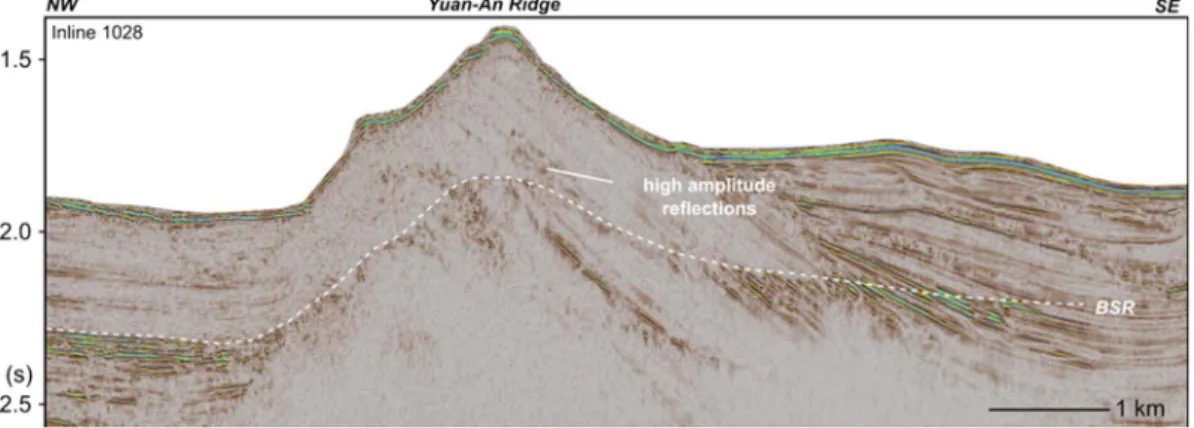
4.2.2. Yuan‐An Ridge
Because of several reported vent sites and strong seismic velocity anomalies, Yuan‐An Ridge has been con- sidered a prime target for gas hydrate exploration (Cheng et al., 2010; Yang et al., 2006). P‐Cable data col- lected at Yuan‐An Ridge (Figure 10) reveal a continuous BSR throughout the 3‐D seismic cube except for an area with poor imaging below the southwestern part of the ridge. The seismic data show a vertical seismic anomaly with subdued reflection amplitudes below a known seep site. Furthermore, there are high‐ Figure 9.Collocated OBS‐derivedPwave velocities (a) and controlled source electromagnetic‐derived apparent electrical resistivities (c) overlain on high‐resolution 3‐D seismic data for Four‐Way Closure Ridge. Panel (b) shows the velocity field derived from the multichannel seismic reflection line that strikes at an angle (Figure 7). Note the very high (2,300 m/s)Pwave velocities and very high (6Ωm) apparent electrical resistivities coinciding with the high‐amplitude reflections in the high‐resolution 3‐D seismic data all pointing to very high hydrate saturations at the core of the anticline. White dots in (b) show mid points for source receiver pairs at depth corresponding to offset where apparent resistivity has been determined and interpolated. OBS = ocean bottom seismometer.
amplitude seismic reflections in the lower part of the GHSZ below the crest of the ridge. The shape and strength of these anomalies are similar to those observed at Four‐Way Closure Ridge. We did not collect OBS or CSEM data in this area, but some OBS data have been collected in the past (Cheng et al., 2010).
5. Discussion
5.1. Systematic Differences in Gas Hydrate Distribution
All observations for the passive margin point toward moderate gas hydrate saturations. As discussed in section 4.1.1 the OBS‐derivedPwave velocities for Formosa Ridge are less constrained than for gas hydrate provinces characterized by stratified sediments (Bünz, 2004) because the chaotic internal structure of the ridge with numerous incised and refilled canyons and sediment waves make it impossible to trace individual phases in the OBS data over large offsets. Nevertheless, the data allow determination of the bulkPwave velo- cities for the lowest part of the gas hydrate stability zone. A velocity of 1,850 m/s at the lower boundary of the gas hydrate stability zone (Figure 5a)fits the observed OBS data best. In the absence of bore hole data the physical properties of the background lithology in the study area are poorly constrained and we cannot con- duct a meaningful inversion of gas hydrate saturation from our data. However, logging while drilling data from well GMGS2‐08 about 60 km west provides valuable constraints on gas hydrate saturation. At GMGS2‐08Pwave velocities of up to 2,700 m/s correspond to hydrate saturations of 60% and 70% of pore fill for vertical and horizontal fracture cementations models, respectively (Wang et al., 2017). These high values are only reached for intervals of few meters thickness, which would not be resolved by our seismic experiments. Therefore, we take the approach to compare our results with those from areas where gas hydrate saturation is well constrained. The study of the Nyegga gas hydrate province of mid‐Norway is argu- ably the best constrained hydrate saturation analysis based on seismic data as both ocean bottom cable data and geotechnical bore hole information exist for this passive margin environment (Bünz, 2004; Bünz et al., 2005). In that kind of geological settingPwave velocities of 1,850 m/s translate into a maximum of 10%
hydrate saturation in the pore space. These saturations occur only in small areas with a diameter of less than 50 m as far as can be determined from the 2‐D seismic data. At GMGS2‐08Pwave velocities of 1,850 m/s also correspond to about 10% and 18% of the porefill, which is broadly consistent with the results from Nyegga but in this instance corroborated by the degassing of pressure cores (Wang et al., 2017). Our forward model- ing of the velocityfield at Formosa Ridge shows seismicPwave velocities up to 1,850 m/s. This would sug- gest that gas hydrate saturation in Formosa is about 10% but generally lower. Obviously, the lower resolution of the OBS‐derivedPwave velocityfield for Formosa Ridge compared to the sonic logs from GMGS2‐08 does not preclude accumulations of higher gas hydrate saturation in the pore space as long as such accumulations are smaller than 200 m in diameter and that these are compensated by a similar‐sized region with lower gas hydrate saturation or the presence of free gas that would yield a combined average velocity of 1,850 m/s.
Figure 10.P‐Cable 3‐D seismic line through Yuan‐An Ridge (location indicated by the dot close to Yuan‐An Ridge in Figure 2). The anticline is formed by a thrust fault and a BSR continues throughout the ridge. Note the high‐amplitude reflections above the BSR in the core of the anticline similar to Four‐Way Closure Ridge. BSR = bottom simulating reflector.
Low gas hydrate saturations at Formosa Ridge are supported by the measured apparent electrical resistivities of less than 3Ωm derived from CSEM measurements. There are few published examples of CSEM experi- ments in gas hydrate regions. Perhaps the best constrained case is Hydrate Ridge for which apparent electri- cal resistivity sections of CSEM data were calibrated by bore hole‐derived gas hydrate saturations (Weitemeyer et al., 2006). Later inversion of the CSEM data found resistivities of up to 3Ωm (Weitemeyer et al., 2010) in an area for which drilling showed gas hydrate saturations of 3–8% of the pore space (Tréhu et al., 2004).
It is reassuring to see that both the OBS and CSEM data independently imply low hydrate saturation below Formosa Ridge, that is, between 5% and 10% of the pore space based on the OBS data and half the electrical resistivity based on the CSEM data (Figures 5a and 5c). We stress however that these values represent the maximum of the average saturation over areas of a few hundred meters, that is, the resolution of the geophy- sical methods. This does not preclude smaller accumulations of higher saturation, for example, along focusedfluidflow pathways. It is thus not surprising that there are mismatches both between the different types of seismic data, that is, OBS seismic velocities versus prestack depth migration seismic velocities and from between the seismic velocities and the CSEM data‐derived electrical resistivities. For example, the low‐velocity zone observed in the OBS data for Four‐Way Closure Ridge is absent in the MCS‐derived velo- cityfield. This could either be due to differences in the ray path, but it is most likely due to the slightly dif- ferent location (Figure 7) and the fact that this anomaly has a limited lateral extent.
Both the OBS and the CSEM data point to much higher gas hydrate saturations in the cores of the active mar- gin anticlines. The bestfittingPwave velocity models for Four‐Way Closure Ridge have a high‐velocity layer at the base of the hydrate stability zone (Figure 9a). ThePwave velocity of this layer increases from 1,900 m/s in the west to 2,200 m/s in the east. As the area is well covered by several OBS and the P‐Cable 3‐D seismic data show that side effects should not play a role as the structure of the ridge is essentially two‐dimensional, these velocities should have an error not greater than ±150 m/s. This is also the error for which we are able to determine misfits between observations and modeling predictions. As for the passive margin, no informa- tion on physical properties exists from drilling. Along with the absence from OBS arrivals from below the BSR inside the anticline this poses the problem that the high velocities may partly be the result of back- ground geology. It is possible that the thrust fault has uplifted more consolidated rocks from below. This is suggested by the trend of higherPwave velocities just below the ridge (Figure 9b). Thus, part of the velo- city increase may be due to this lithological change. Therefore, it is impossible to invert for precise hydrate concentrations. However, it is instructive to compare the derived velocities with better constrained cases to estimate the possible range of hydrate saturations. Comparison of the predictions of several effective med- ium theories with bore hole‐derived hydrate saturation and logging‐derivedPwave velocities shows that Pwave velocities of 2,350 m/s translate into hydrate saturations between 30% and 70% assuming a contact model with hydrate as part of the solid and that porosities between 0.4 and 0.7 are realistic for Four‐Way Closure Ridge (Chand et al., 2004). This is in agreement withfield measurements made at Daini‐Atsumi Knoll (Fujii et al., 2015). At Daini‐Atsumi KnollPwave velocities above 2,500 m/s only occur in sandy inter- vals and at hydrate saturations above 50%. However, it is noteworthy that such high values are only found over intervals that are below the resolution of our OBS data evaluation, that is, between 310 and 336 m below the seafloor. This implies that the hydrate accumulations at Four‐Way Closure Ridge are possibly more extensive and concentrated than those at Daini‐Atsumi Knoll.
The CSEM data‐derived apparent electrical resistivities for Four‐Way Closure Ridge reach up to 6Ωm and coincide with the highestPwave velocities and the high‐amplitude seismic reflections observed in the P‐ Cable 3‐D seismic data for the core of the anticline. The electrical resistivity anomaly splits up into a western and an eastern branch that extend from the base of the hydrate stability zone to approximately 30–50 m below the seafloor. Such high apparent resistivity anomalies have not been observed in any previous CSEM experiments conducted in hydrate provinces. Therefore, their interpretation is difficult. Archie's law (Archie, 1942) can be used to derivefirst estimates for the hydrate concentration from the apparent resis- tivitiesρ:
ρ¼aϕ−mS−nρwater
witha, n, andmempirical values,Φporosity, andSsaturation. Since porosity and lithology information is
missing, this estimation can only be done by assuming plausible ranges for the governing unknown para- meters (porosityΦ= 55–65%; cementation exponentm= 1.6–2.0) as well as reasonable values for para- meters of lesser significance (saturation exponentn= 1.9386). For afluid conductivity of 3.17 S/m, which was measured by a CTD probe during the experiments, these parameters yield gas hydrate saturations between 51% and 61% (ρa= 4Ωm) and 60–68% (ρa= 6Ωm; Figure 9). The true electrical resistivities and consequently the hydrate saturations, which can be derived from a full inversion of the data, could be even higher than the apparent resistivity values derived here, as has been shown for CSEM data from the Gulf of Mexico (Constable et al., 2016). One could also consider the electrical resistivity measured in bore hole data for the Daini‐Atsumi Knoll. Here, 6‐Ωm resistivity in the bore hole corresponds to 20–40% hydrate satura- tion (Fujii et al., 2015). It is interesting to note that the high apparent electrical resistivities are also observed under the western part of Four‐Way Closure Ridge where the OBS data show only moderately increasedP wave velocities of approximately 1,900 m/s, while the reflection seismic character appears unaltered. The data provide no conclusive reason for this. A possible explanation is that high apparent electrical resistivities shown in the CSEM data may be caused by gas hydrate or free gas while the velocity response is very differ- ent (high velocities for hydrate and low velocity for free gas). Possibly, the western part of the anticline con- tains not only hydrate but also significant amounts of free gas which would reduce the overallPwave velocity from 2,200 ± 150 to 1,900 m/s. The only observable difference in the configuration of seismic reflec- tors in the eastern and western part of the ridge is a band of low‐amplitude reflections below the high‐
amplitude reflectors in the eastern part of the ridge, which is not visible in the western part. Possibly hydrate saturations are highest in this zone immediately above the BSR (Figure 8b). We note, however, that the high electrical resistivities could also be caused by other processes that reduce the amount of saline pore water.
These include the precipitation of authigenic carbonates consumption of pore water for hydrate formation, that is, dry pores, or compaction of sediments that have been uplifted later on. Without drilling information, it is not possible to constrain this further.
In summary, both the OBS data and the CSEM data at Four‐way Closure Ridge suggest much higher, that is, 20–50%, average hydrate saturation in the pore space compared to Formosa Ridge, where average hydrate saturation does not exceed 10%. In spite of the limitations in determining hydrate saturation in the pore space due to the complex geology of Formosa Ridge and the shortcomings involved in using Archie's equa- tion, thesefindings are qualitatively robust.
This trend is supported by published information from other subduction zones. OBS data collected at Yuan‐ An Ridge (Liu et al., 2005) confirm an increase of seismic velocity up to 1,950 m/s above the BSR, but they do not provide detailed information on lateral velocity variations. These authors arrive at hydrate saturations between 5% and 25% of the pore space. Also, at Yuan‐An Ridge we observe numerous high‐velocity seismic reflections in the P‐Cable reflection seismic data immediately above the BSR (Figure 10). Considering that similar high‐amplitude anomalies have been discovered in the cores of anticlinal ridges in the subduction zones of Makran off Pakistan (Smith, McNeill, et al., 2014), in the Nankai Trough off Japan (Fujii et al., 2015), and on New Zealand's Hikurangi margin (Crutchley et al., 2015), it seems that high gas hydrate saturations linked to high‐amplitude seismic reflectors are a typical feature of subduction zone hydrate accu- mulations and that there must be mechanisms that affect only the active margin and that allow large amounts of gas to enter the gas hydrate stability zone and form high saturation deposits.
5.2. Controls on Gas Hydrate Formation
Evidence for neotectonic activity on the passive margin is restricted to the shelf area (Figures 4 and 6). While normal faults offset the shallow strata down to 4‐s TWT and seem to be linked to old structures that devel- oped during formation of the northern margin of the South China Sea (Lin et al., 2008) such faults are absent in the gas hydrate province south of the shelf break. Even if minor faults are not resolved by the existing reflection seismic data because of incomplete coverage or poor data quality, it is clear that tectonic structures do not provide pathways for widespreadfluid advection from the Mesozoic prerift sediments that are buried by approximately 4 km of subsequently deposited sediments. The reflection seismic data do not reveal other fluid pathways such as pipes or chimney structures (Karstens & Berndt, 2015) either. The absence of impor- tant focusedfluidflow pathways is supported by the high‐resolution 3‐D seismic data, which show thatfluid focusing occurs at the depth of the BSR where pipe structures originate and penetrate through the overlying contourite sediments (Figure 4b; Hsu et al., 2017). We propose that focusing at BSR level is a direct result of
the presence of gas hydrates in the pore space, which reduces the permeability and leads to pore pressure buildup below the highest points of the BSR until hydrofracturing generates focusedfluidflow pathways and bleeds off the pore pressure (Bünz et al., 2003). Thermogenic gas exists in prerift sediments below the outer shelf of the Taiwan Strait where it has been exploited as a gas reservoir in theFfield (Lin et al., 2008), but there is no seismic or bathymetric evidence forfluid migration into the hydrate province or that any of the rift‐related faults extend out beyond the shelf break. It is likely that the vicinity of the subduction zone will have an effect on stress regime also in the passive margin, but this effect seems to be minor as it does not lead to faulting that could be observed in the 3‐D seismic data. The absence of a thermogenic gas source is supported by seafloor gas sampling at Formosa Ridge, which did not detect any thermogenic gas (Feng & Chen, 2015). However, as the gas composition on the passive margin of the SCS has only been sam- ple in very few places and because these measurements may still be overprinted by secondary microbial gas formation and gas hydrate dynamics, it is quite possible that gas of thermogenic origin may be discovered in this area in the future.
In contrast to this the active margin is characterized by numerous thrust faults and blind thrust faults that lead to anticlinal ridges at the seafloor. Thrust faults in accretionary prisms have been shown to be efficient pathways forfluids that rise from the décollement both by direct observation (Park et al., 2002) and through geochemical evidence for pastfluid migration (Travé et al., 1997). Generally, cold seeps in subduction zones are found on the tops of anticlinal ridges and not at the fault trace on the seafloor (Chuang et al., 2010;
Klaucke et al., 2015) at the foot of the anticlinal ridges. The same observation has been made for the Makran accretionary prism off Pakistan (Smith, McNeill, et al., 2014). Analysis of the seismic reflection coef- ficient of reflections from thrust faults in the Makran accretionary prism suggests that at least the upper few kilometers of the faults act asfluid pathways. In the case of the Makran accretionary prism seismic data sug- gest that the deeper part of the prism is already dewatered to a large extent and littlefluid migrates through the deepest 2–3 km of the accretionary prism. This may be the result of particularly thick sedimentary over- burden in excess of 7 km. Importantly, the presence of high permeability pathways in the thrust faults still facilitatesfluid focusing although there is not a prolificfluid source such as an active décollement. Off Makran thefluids migrating along the faults seem to be sourced from biogenic gas production in the upper 2–3 km of sediments, while the seeps on the active margin off Taiwan show admixing of thermogenic methane to the otherwise biogenic signatures (Chuang et al., 2010) withδ13C values as high as−28.3‰.
The strongest thermogenic signatures are observed above mud volcanoes near the coast.
Given the same sedimentation history of the active and passive margins, the presence and absence of major fluid pathways from depth is the most obvious difference in geological setting that may explain the widely varying predicted gas hydrate saturations. We propose that strong advection of gas from greater depth is the main difference between the gas hydrate systems on the passive and active margins. The geochemical indications for the advection of thermogenic gas suggest that, at least, part of this gas is coming from the depth of the décollement where it is formed by kerogenesis. This alone, however, would not explain why high hydrate saturations are also found in the lower, western part of the accretionary prism where the geo- chemical signatures only show minor admixture of thermogenic gas. We postulate that the faults are also important for higher hydrate saturations because they provide drainage pathways for the deeper region of the biogenic gas production window (Figure 11). Data from Makran seem to indicate that this can be suffi- cient for generating high hydrate saturations at the surface (Smith, McNeill, et al., 2014).
5.3. Influence of Gas Hydrates on the Fluid Flow System
Both on the passive margin and on the active margins we observe focusing offluid migration at the base of the hydrate stability zone suggesting that the presence of gas hydrate influencesfluid migration. We observe that pipe structures rise from the highest points of BSRs. As mentioned above, this spatial relationship has been observed in many gas hydrate provinces such as Nyegga (Bouriak et al., 2000; Bünz et al., 2003; Plaza‐ Faverola et al., 2011), Opouawe Bank (Plaza‐Faverola et al., 2012), Vestnesa (Petersen et al., 2010), and Hydrate Ridge (Crutchley et al., 2013). Analysis of these pipe structures has shown that their formation is consistent with pore pressure build up due to reduced permeability and subsequent hydrofracturing. The locations of the pipe structures below the southern summit of Formosa Ridge and the summit of Four‐ way closure Ridge suggest that they have formed in the same way. Thus, their presence can be taken as evi- dence for gas hydrate at the base of the hydrate stability zone but should not be seen as an indication for
particularly high hydrate saturation at depth as this process can also be active at saturations below 10% of the porefill (Bünz et al., 2003).
The absence of seeps at the fault trace of the thrust faults at the seafloor is striking, in particular as the same observation has been made in other subduction zones where gas hydrates exist (Barnes et al., 2010; Smith, McNeill, et al., 2014). Instead, most seeps occur above pipe structures at the apices of the anticlinal ridges.
We propose that this is the result of a deviation offluid migration due to hydrate formation in the thrust fault where it intersects the base of the hydrate stability zone. In our interpretation, advected methane will initi- ally form a hydrate plug and reduce the permeability of the thrust below the permeability of the surrounding sediments. In this case, thefluids would be deflected upward along the base of the BSR toward the core of the anticline. Gas will then accumulate below the highest point of the BSR and overpressure will build up due to the gas buoyancy.
5.4. Implications for Gas Hydrate Resource Estimates
Both our OBS and CSEM data and the OBS data of previous studies (Schnurle et al., 2005) show that gas hydrate saturations are significantly higher in the core of the Yung‐An Ridge and Four‐Way Closure Ridge anticlines compared to Formosa Ridge, although admittedly this is just one of many ridges on the pas- sive margins of the South China Sea and drilling has shown that at least locally higher gas hydrate satura- tions may occur (Wang et al., 2017). If the congruence of high‐amplitude reflections immediately above the BSR in the reflection seismic data and the high‐velocity regions in the OBS data is indeed caused by the presence of large amounts of hydrate it is possible to use the high‐amplitude reflections above the BSR as a proxy for high saturation gas hydrate deposits. The geophysical and bore hole studies at Daini‐ Atsumi Knoll in the Nankai Trough (Fujii et al., 2015) support this inference, as do studies in the Gulf of Mexico (Boswell et al., 2012, 2015) and offshore New Zealand (Crutchley et al., 2015). In this case the gas Figure 11.Schematic distribution offluid advection patterns. While biogenic gas production fuels the gas hydrate system of the passive margin (top), the thrust faults of the active margin funnel both biogenic and thermogenic gas to the base of the gas hydrate stability zone where it forms gas hydrate (bottom). Regional gas hydrate deposits on the active margin reduce the permeability at the base of the hydrate layer, deflecting gas upslope to the core of the anticlines where the highest gas hydrate saturations are observed. BSR = bottom simulating reflector.