AVM and High Dimensional Data - Do Ridge, the Lasso or the Elastic Net provide an 'automated' solution?

Published by

DFG Research Unit 2569 FORLand, Humboldt-Universität zu Berlin Unter den Linden 6, D-10099 Berlin

https://www.forland.hu-berlin.de

Tel +49 (30) 2093 46845, Email gabriele.wuerth@agrar.hu-berlin.de

Ag ricul tural Land M arkets – Effi ciency and Regu la ti on

AVM and High Dimensional Data - Do Ridge, the Lasso or the

Elastic Net provide an

`automated' solution?

Nils Hinrichs, Jens Kolbe , Axel Werwatz

FORLand-Working Paper 2 2 (2020)

AVM and High Dimensional Data – Do Ridge, the Lasso or the Elastic Net

provide an ‘automated’ solution

Nils Hinrichs, Jens Kolbe and Axel Werwatz

∗Institut f¨ur Volkswirtschaftslehre und Wirtschaftsrecht, Technische Universit¨at Berlin, Straße des 17. Juni 135, 10623 Berlin, Germany, jkolbe@tu-berlin.de and axel.werwatz@tu- berlin.de.

Abstract

In this paper, we apply Ridge Regression, the Lasso and the Elas- tic Net to a rich and reliable data set of condominiums sold in Berlin, Germany, between 1996 and 2013. We their predictive performance in a rolling window design to a simple linear OLS procedure. Our results suggest that Ridge Regression, the Lasso and the Elastic Net show po- tential as AVM procedures but need to be handled with care because of their uneven prediction performance. At least in our application, these procedures are not the ‘automated’ solution to Automated Valuation Modeling that they may seem to be.

Keywords: Automated valuation, Machine learning, Elastic Net, Fore- cast performance

JEL Classification: R31, C14

1 Introduction

Automated Valuation Models (AVMs) use recorded transaction or listing in- formation to fit a statistical model of the relationship between prices and characteristics of properties. Once the model is fitted, the market value of any property with given characteristics can easily be predicted. The challenge lies in the modeling stage. It is exacerbated by the ‘nature’ of properties and property data. Properties are very heterogeneous and their value depends on a multitude of factors. Thus, to be reasonably accurate, AVMs need to be based on data with detailed information on property characteristics. At the same time, turnover in property markets is typically rather low. Statistically speak- ing, this translates into a regression problem with relatively few observations but a relatively law large set of predictors. Very flexible and very data hun- gry models such as nonparametric regression or neural networks thus quickly run into the ‘curse of dimensionality’ in this situation: their estimates of the price–characteristics relationship become very imprecise and their predictions therefore can become quite inaccurate. Thus, simply ‘letting the data speak’

is not a real option in AVM regression modeling.

In this paper, we thus follow a different modeling approach. We focus on flexible parametric regression models and estimate them by constrained least squares from a rich and reliable data set of condominium transactions. By working with a basis expansion of the set of original property characteristics, these models have the ability to adapt quite flexibly to the relationship of theses characteristics and the transaction price contained in the data. The two constrained least squares estimators, –ridge regression and the LASSO– , make sure that this flexibility does not get out of control. They both ‘regu- larize’ the problem by constraining the total size of the regression coefficients.

By shrinking some regression coefficients (ridge regression) or setting some to zero (LASSO) the procedures make sure that the coefficients of the im- portant relationships can be estimated precisely and that precious degrees of freedom are not wasted on coefficients of unimportant predictors. Which co- efficients are constrained, and thus which predictors are deemed unimportant,

is determined in a data-driven, automated way – thus entirely in the spirit of automated valuation.

We apply ridge regression and the LASSO to a data set containing detailed information on all condominiums sold between 1996 and 2013 in Germany’s capitol Berlin. All information is retrieved from the actual sales contracts and can be regarded as reliable. We thus imagine the situation of an AVM service that delivers property valuations not to the general public but to professional customers such as mortgage lenders who demand and reward accuracy. Such an AVM service needs rich data and may even merge information on a given property from various databases – for instance, by enhancing records on a specific property with indicators on upkeep derived from images of the prop- erty or indicators on neighborhood amenities from a web mapping service. In short, while our data is quite detailed, the challenge that is at the heart of our approach (the number of observed properties being small relative to the dimension of the set of observed determinants) is likely to be even more intense in other current and future AVM applications.

The remainder of this paper is organized as follows. Section 2 discusses our methodology for developing our AVM regressions and how we will be assess- ing and comparing their performance. Section 3 presents the data. Section 4 explains the model specification results and the performance assessment ob- tained from the validation step. Section 5 concludes. Details of the analysis are relegated to the Appendix.

2 Methodology

2.1 Theoretical Framework

The aim of AVM is providing model-based predictions of the market value of a residential property. The market value is the price one should expect in an arm’s-length transaction between informed and willing buyers and sellers.

We denote this price as P_jt for property j at time t. This value depends on

the property’s structural and location characteristics. Those that are observed in the AVM’s data base are summarized in the vector xjt. In our data set, x_jt includes –among other things– a condominium’s living space, number of bedrooms or location within the building.

A reasonable criterion for assessing predictive quality is the mean squared prediction error. It is well-known that in this case the optimal predictor of P_jt, given x_jt, is the conditional expectation E[Y_jt|x_jt]. The goal of an AVM is thus to provide a good estimate of this conditional expectation. Denote such an estimate of a candidate model k as ˆE[Yjt|xjt] = ˆmk(xjt). For any estimated candidate model, the mean squared prediction error for a property with characteristics x_jt can be decomposed as (Hastie et al. (2009), p. 223) E[(Pjt−mˆk(xjt))²|xjt] = Var(Pjt|xjt) + E{mˆk(xjt)−E[Pjt|xjt]}² + V ar[ ˆmk(xjt)] (1)

The first part on the right hand side of equation (1) is the variance of prices of properties with the given the bundle of characteristics xjt. It does not depend on ˆm_k(x_jt) and is thus not affected by the quality of any candidate AVM. It is therefore often referred to as the ‘irreducible error’. However, enlarging the set of features included inx_jt willin general decrease this conditional variance and the mean squared prediction error. It explains why there is a strong incentive for AVM providers to collect detailed information on properties. It can be expected that in the future the dimension of the feature vector x_jt will continue to grow. The second part of the decomposition is the squared bias of the estimated candidate model ˆmk(xjt). This term can itself be decomposed into two parts, the estimation bias and the model bias, highlighting the fact that the quality of any AVM model has two key aspects: the quality of the functional form assumptions of the model and the quality of the estimation procedure used to fit the model. The latter, the estimation quality, takes center stage in the third and final component of (1), the variance of the candidate model estimator.

In the remainder of the paper, we assume that the set of available covari- ates xjt may be large but that it is fixed at the moment. Hence, the first term of the decomposition (1) then is indeed ‘irreducible’ and AVM prediction

quality entirely hinges on keeping the second and third terms as low as pos- sible. Therein, however, lies a well-known trade-off: candidate models with flexible functional forms keep the model bias low but often suffer from large estimation error because of their complexity. The relatively few parameters of parsimonious candidate models, on the other hand, can typically be estimated precisely but their restrictive functional forms may result in a large model bias.

The key to AVM is thus to find a model that delivers the best compromise between bias and variance.

We illustrate this trade-off and our candidate solutions in a highly simplified situation. Suppose that living space were the only continuous characteristics, that there were only two locations A and B and only two time periods, 1 and 2.

Then an extremely simple candidate model is the following linear, additively separable model (LASM)

m_LASM(x_jt) =β₀ + β₁space_jt + β₂loc.Bjt + β₃period2_jt (2) where loc.B and period2 are accordingly defined dummy variables. The model presupposes, for instance, that the effect of space is the same at both locations and in both time periods and is linear (i.e., independent of its own level). This functional form strongly restricts the ability of the model to adapt to the data. It is thus likely to suffer from a substantial model bias. The four parameters of the model, however, are easily estimated by least squares.

Indeed, least squares will provide unbiased estimates of the model parameters in (2).¹ Estimation bias will thus be zero in this case and the squared bias term in (1) is entirely due to the model bias for this candidate model. Because of its simplicity and parsimony, estimation variance, the third term in (1), will be very small. A particularly clear expression of this can be obtained if the variance of ˆm_LASM(x) =x^Tβˆ^LS is not considered at a particular property with characteristics x_jt (as in (1)) but instead averaged over the properties in the

1More precisely, least squares will provide unbiased estimates of the parameters of the Best Linear Predictor, as which we implicitly define 2. See Hastie et al. (2009), p. 19.

training data:

1 n T

n

X

i=1 T

X

t=1

Var( ˆm_LASM(x_it)) = 1 n T

n

X

i=1 T

X

t=1

Var(x^T_itβˆ^LS) = σ²

n T p (3) This expression, which holds under the assumption of a constant conditional variance Var(P_jt|x_jt) = σ², shows that the estimation variance is linearly in- creasing in the number of regression parameters p+ 1. The latter is also the degrees of freedom of this procedure.

At the other end of the model complexity spectrum is the nonparametric regression model. In our simplified illustration, it is given as

m_{N P M}(x_jt) =m(space_jt,loc.Bjt,period2_jt) (4) This model imposes no parametric functional form on the data and allows for arbitrary nonlinear effects of continuous regressors like space and for arbi- trary interactions among the effects of all explanatory variables. This highly flexible model thus has very little if any model bias. It can be estimated by lo- cal smoothing procedures like kernel regression, k-nearest neighbor regression or smoothing splines. However, regardless of which estimator is applied, its variance increases dramatically with p for a given sample size, the well-known

‘curse of dimensionality’.

An alternative model, that allows for a nonlinear effect of floor space (via a cubic polynomial) and an interaction between floor space and location in a parametric way is given by:

ˆ

m_{F LM}(x_jt) =β₀ + β₁space_jt + β₂space²_jt + β₃space³_jt + β₄loc.Bjt + β₅period2_jt

+ β6loc.Bjt×space_jt

+ β₇loc.Bjt×space²_jt + β₈loc.Bjt×space³_jt

This ‘compromise’ model is similar in spirit to the very flexible parametric model we actually apply below and which we describe in the following sub-

section. It is substantially more flexible than the simple additively separable linear model, reducing the risk of a large model bias. On the other hand, it is linear in the parameters (thus the subscript F LM for flexible linear model) and is thus easily estimated by least squares. Because it has eight param- eters (rather than just four), its variance will be slightly larger that that of

ˆ

m_LASM(x_jt and may thus offer a better bias-variance balance. In our empirical work, we take model (2.1) to its limits with regard to flexibility by considering nonlinear basis functions of the original continuous regressors and by including almost all possible interactions. We then use three constrained least squares procedures, ridge regression, the Lasso and the Elastic Net, to automatically shrink estimated parameters in order to keep the variance in check. The main advantage of this approach is that it offers an automatic, data-driven and com- putationally tractable solution to the key question in AVM specification search:

arriving at an estimated model that presents a good compromise between bias and variance and is thus a sound basis for fast and accurate valuations.

2.2 A very flexible parametric model

We will now describe the details of our approach. Suppose first that there were only continuous property features, such as floor space, and that for each transacted property we would observe p such characteristics: X₁, X₂, . . . , X_p. In order to allow for enough flexibility of the functional forms of the relation- ships between price and these continuous characteristics, we employ a basis expansion in these variables. The model for the conditional mean of prices becomes:

m_{F LP}(x_jt) =β₀+

M

X

m=1

β_mh_m(X_1t, . . . , X_pt) (5) This model is linear in the parameters β₁, . . . , β_M but via the basis functions h_m(X₁, . . . , X_p) we allow for non-linearity. We use the following basis func- tions:

h(X1t, . . . , Xp) =







t_θ(X_j) for each j and each θ t_θ1(X_j)·t_θ2(X_k) for each j and k if θ₁ 6=θ₂

(6)

where t_θ(X) denotes a Box-Cox-transformation of the following form²

t^(θ)_j =







x^θ_j for θ ∈ {±2,±1,±0.5}

log(x_j) for θ= 0

. (7)

That is, the first type of basis function considers one explanatory variable at a time, transformed in one of the seven possibilities offered by the class of Box-Cox-transformations. Since we have p = 18 continuous characteristics³, this results in 18 × 7 = 126 basis functions of the form h(X₁, . . . , X_p) = tθ(Xj). It is easiest to think about them as a set of transformed versions of the original explanatory variables. Using space to illustrate, the model will include space⁻²,space⁻¹,space^−0.5,log(space),space^0.5,space and space², each with its own β coefficient.

The second type of basis functionsh(X1, . . . , Xp) =tθ1(Xj)·tθ2(Xk) consid- ers interactions between any of the 126 Box-Cox transformed original explana- tory variables. As an example,t_θ1=0.5(space)·t_θ2=0(age) =space^0.5×log(age) is a standard interaction terms of two transformed versions of floor space and age of the property. Products of transformed versions of the same explanatory variable are also considered, provided the transformation parameters differ be- tween the two factors. Using X_j =space to illustrate,t_θ1=0.5(X_j)·t_θ−2(X_j) = space^0.5×space⁻² =space^−1.5is such an example.⁴ Because we start with 126 transformed variables, this gives us a total of ¹²⁶₂

= 7875 such product vari- ables.⁵ 54 of these are constant (for example the interactionX_j²·X_j⁻² = 1) and 72 duplicate an already existing transformed variable (e.g. X_j¹·X_j^−0.5 =X_j^0.5).

These need to be removed, leaving us with 7,749 additional variables in the model from the interaction terms. Hence, the basis expansion from the con- tinuous regressors gives a total of 126 + 7749 = 7875 terms in (5).

2Box and Cox, 1964

3A detailed description of the continuous and discrete characteristics in our data is given in section 3. We refer to them synonymously as ‘characteristics’, ‘covariates’, ‘features’,

‘explanatory variables’ and ‘predictors’.

4To the contrary, tθ_1=0.5(Xj)·tθ_0.5(Xj) =space^0.5×space^0.5 =space¹ is nota proper product as both factors use the same transformation parameter, i.e. θ1=θ2= 0.5.

5The interactions also widen the spectrum of polynomials included for each continuous covariate, which now also includex^θ forθ∈ {±3,±2.5,±1.5}.

Next, we consider the 81 discrete, binary features in our data which we generically denote as Dj. They include dummy variables for time periods (years) and regions (districts of Berlin). They are all entered with their own coefficient. Moreover, all pairwise interactions are also created for them, lead- ing to ⁸¹₂

= 3,240 additional binary variables of the form D_jk = D_j ·D_k for all j 6= k.⁶ While these interactions also serve the purpose of enhanced model flexibility, they are easily interpretable and allow for different valua- tions regarding certain characteristics across time, space and in combination with other characteristics.⁷ Our flexible parametric model now reads:

m_{F LP}(x_jt) = β₀+

7875

X

m=1

β_mh_m(X_1t, . . . , X_pt)) +

18

X

j=1

β_j^dD_jt + X X all^j,k:j6=k

β_j,k^d D_jt·D_kt

Moreover, we include pairwise interactions between the 81 uninteracted bi- nary variables and the 18 untransformed continuous variables, creating 1,458 additional covariates. The interactions, again, further enhance model flexibil- ity by allowing for different effects of continuous regressors for instance across time and space. Our count of predictors and parameters on the right hand

6Because certain characteristics never occur simultaneously in the data, some of these binary interactions are zero for all observations and consequently dropped in the estimation stage.

7For example, the value of basement storage space may be different across Berlin’s dis- tricts or may have changed over time. Also, certain characteristics may lose or gain value in combination with others. Paying a premium for basement storage space may be less attractive if the apartment itself contains a storage rooms.

side of our model now is 7875 + 81 + 1458 = 9414 and the model becomes:

m_{F LP}(x_jt) = β₀+

7875

X

m=1

β_mh_m(X_1t, . . . , X_pt)) +

81

X

j=1

β_j^dD_j + X X allj,k:j6=k

β_j,k^d D_jt ·D_kt

+

81

X

j=1 18

X

k=1

β_j^dxD_jt·X_kt (8)

At last, we include a set of detailed binary indicators for a property’s loca- tion and time of sale that we do not interact with other discrete or continuous regressors. Specifically, these are dummy variables indicating the borough (German: Ortsteil) of a property and its quarter of sale.⁸ We do this because location is typically seen as one of the most important determinants of a prop- erty’s value and because we use data from several years of a dynamic property market. On the other hand, it is neither plausible nor feasible to let the effect of, say, floor size on property prices change every quarter or every borough.

This is why we include the more crudely coded year dummies and district dummies as part of the fully interacted binary indicators described in the pre- vious paragraph and the more finely graded borough and quarter dummies as a separate group of un-interacted indicators that close out the specification.

Thus, the final model is

8There are 96 boroughs in Berlin and 40 quarters in each estimation sample.

m_{F LP}(x_jt) = β₀+

7875

X

m=1

β_mh_m(X_1t, . . . , X_pt))

+

81

X

j=1

β_j^dDj + X X all^j,k:j6=k

β_j,k^d Djt ·Dkt

+

81

X

j=1 18

X

k=1

β_j^dxD_jt·X_kt

+

95

X

j=1

β_j^bB_jt+

39

X

j=1

β_j^qQ_jt (9)

At this point, 9,549 covariates are available for predicting the price. Clearly, this is a very flexible model but, in terms of (3), a specification that is likely to suffer from very imprecise estimates, if it can be fit at all. A may thus be gained in estimation precision and therefor prediction accuracy if the model complexity can be reduced in the right way. This is what Ridge regression and the Lasso try to achieve. To simplify the notation for our discussion of these two procedures, we rewrite the model simply as

m_{F LP}(x_jt) =

M

X

m=1

β_mz_m,jt (10)

where all predictors on the right hand side of (9) have been consecutively num- bered and are denoted as z_m with the corresponding consecutively numbered coefficients simply denoted as β_j, j = 1, . . . , M = 9549

2.3 Regularization

The model described in the previous section can, in principle, adapt very flex- ibly to the patterns in the data. This flexibly comes at the price of a huge number of parameters. Fitting this linear model via Least Squares results in an estimation bias of zero. However, this may neither be computationally

possible not statistically desirable.⁹ Indeed, there may be a sizeable gains in terms of variance reduction by using a biased estimator that ‘regularizes’ the complexity of the model by minimizing the sum of squared residuals subject to a constraint on flexibility. This is achieved by shrinking the coefficients of

‘unimportant’ regressors. From (1) above it is clear that such a biased but less variable estimator may result in an overall reduction of the expected squared prediction error. Indeed, the question of how many and which regression co- efficients should be shrunk can be seen as synonymous with variable or model selection. Ridge regression, the Lasso and the Elastic Net offer an objective answer to this question, basically by shrinking coefficients of regressors that provide little information either because they hardly vary across properties or are highly correlated with other regressors and thus provide no additional information. It is reasonable to assume that both phenomena occur in the problem at hand. The correlation between several characteristics in the orig- inal dataset is considerable, for example between the size of all residential and shared units and the size of all residential units. The transformations and interactions described above only aggravate the problem. If, for instance, a continuous variable is multiplied by a dummy variable that predominantly contains the value 1, this new variable is a nearly perfect copy of the orig- inal continuous feature. Although only nonlinear transformations are used, correlations between covariates and their transformations can still be high.

Since the only variables excluded from the analysis are those unusable due to missing values or purely administrative, redundant information is potentially contained in the data which motivates the need for regularization.

2.4 Ridge regression

Ridge regression, introduced by Hoerl and Kennard (1970), regularizes the problem by imposing penalties on the size of the estimated parameters, result- ing in a unique solution even if the regressor matrix is not of full rank. The ridge estimate for the parameter vector β is found by minimizing the residual

9Computationally, if the number of parameters exceeds the sample size, there is no unique least squares solution. See Fahrmeir et al. (2009), p. 61.

sum of squares, subject to the sum of the squared parameters not exceed- ing a specified threshold t. To make the parameters independent of scale, all covariates are standardized.

βb^R= arg min

β

( _n X

i=1 T

X

t=1

(P_it−β₀−PM

m=1β_mz_m,it)² )

s.t.

M

X

m=1

β_m² ≤t (11)

Equivalently, this may be written as (citehastie2009, p. 63),

βb^R= arg min

β

( _n X

i=1 T

X

t=1

(P_it−β₀−PM

m=1β_mz_m,it)²+λPM m=1β_m²

)

, (12)

since for any threshold t ≥ 0, a tuning parameter λ ≥ 0 exists, which results in exactly the same estimator. The choice of the tuning parameter controls the amount of parameter shrinkage. Choosing a very large threshold t results in equivalence between Ridge regression and OLS. The smaller t (or, equivalently, the larger λ), the more shrinkage is performed.¹⁰

In matrix notation, the Ridge solution is given by

βb^R = (Z^TZ+λI)⁻¹Z^Tp . (13) wherep is the (centered) vector of prices and the regressor matrix Z does not include a column of ones for the intercept and standardized versions of the z_m, m = 1, . . . , M. Ridge estimation is biased towards zero. The size of the bias depends on the choice of the tuning parameter λ. We choose λ by cross validation. The negative effect of introducing a bias may be outweighed by the fact that Ridge regression, in general, has a lower estimation variance than unconstrained least squares, see Zou and Hastie (2005).

10No restriction is imposed on the parameter β0 to make the procedure independent of the particular level of the average price, see Hastie et al. (2009), p. 64. In fact, centering the vector of prices allows estimation of the model without an intercept and recovering it afterwards.

Graphically, the ridge constraint forms a circle in a two-parameter problem (see the red circle in Figure 1). The Ridge solution is the smallest value of the residual sum of squares function within that circle. The picture illustrates why the Ridge estimator has, in general, a smaller variance than unconstrained least squares (OLS). The OLS solution can, depending on the data, lie anywhere in the plane spanned by β₁ and β₂, while the Ridge solution is guaranteed to lie within the depicted circle.¹¹ While Ridge regression may thereby achieve a better bias-variance compromise and thus a superior predictive performance, it does not perform variable selection as it generally does not shrink coeffcients all the way to zero. This is done by the Least Absolute Shrinkage and Selection Operator (Lasso).

2.5 Lasso regression

Lasso employs a slightly altered constraint which limits the sum of theabsolute values of the coefficients. This ensures that not only are coefficients shrunk but some are set to exactly zero, turning the procedure into a ‘Selection Operator’.

The Lasso was first introduced in Tibshirani (1996) to combine the favorable properties of Ridge regression with the desire to find an interpretable model.

The Lasso estimator is defined by

βb^L= arg min

β

( _n X

i=1 T

X

t=1

(P_it−PM

m=1β_mz_m,it)² )

s.t.

M

X

m=1

|β_m| ≤t

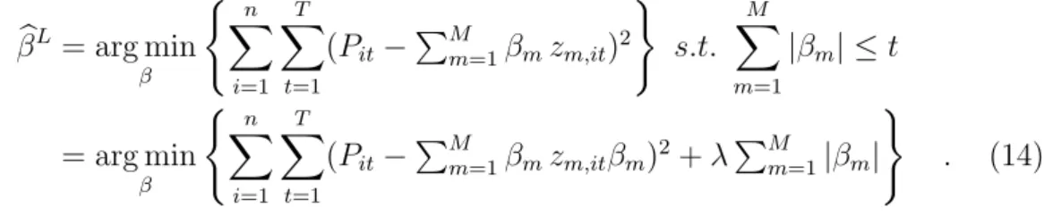
= arg min

β

( _n X

i=1 T

X

t=1

(Pit−PM

m=1βmzm,itβm)²+λPM

m=1|βm| )

. (14) No closed form solution exists for the estimator in case of more than one predictor, but the problem is convex and a solution can be found iteratively.

Figure 1 shows that the constraint of the Lasso has the form of a diamond with edges even for a two parameter problem. If the solution occurs at such an edge, a parameter is set to zero, resulting in variable selection. The number of

11Ridge regression is able to find a solution for M > N problems and handles highly correlated variables more effectively than unconstrained least squares.

edges rises exponentially. For two parameters, the depicted diamond has four edges. For three parameters, the constraint region is a cube with eight edges.

Each additional parameter doubles the number of edges, creating numerous opportunities for parameters to be set to zero¹². The amount of parameter shrinkage and variable selection depends on the choice of the tuning parameter.

If a large enough thresholdt(or, equivalently, a small enough tuning parameter λ) is chosen, the OLS solution falls within the depicted diamond and neither shrinkage nor selection are performed. A large value of λ or a small threshold t lead to substantial shrinkage with many parameters being set to zero. We select λ by cross validation.

The Lasso exhibits several shortcomings, though. Its nonzero parameter estimates tend to be biased towards zero. Also, when dealing with highly correlated variables the Lasso performs poorly. Slight changes of the tuning parameter λ can have wild effects on estimated parameters, and from a group of highly correlated variables, the Lasso tends to select some and discard others in a rather random fashion. The Elastic Net, a Generalization of the Lasso tries to overcome these shortcomings at the cost of an additional tuning parameter.

2.6 Elastic Net regression

The Elastic Net (introduced by Zou and Hastie (2005)) is a compromise be- tween Ridge and Lasso. Its constraint on the parameters is a mixture between the L₁ penalty of Lasso and the L₂ penalty of Ridge regression. For any

12See Hastie et al. (2015), p. 12.

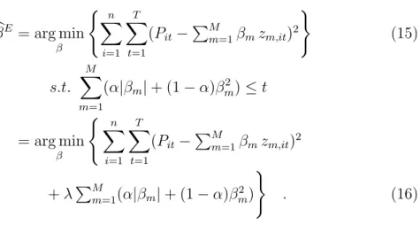
α ∈[0,1] the Elastic Net estimator is defined as

βb^E = arg min

β

( _n X

i=1 T

X

t=1

(P_it−PM

m=1β_mz_m,it)² )

(15)

s.t.

M

X

m=1

(α|β_m|+ (1−α)β_m²)≤t

= arg min

β

( _n X

i=1 T

X

t=1

(P_it−PM

m=1β_mz_m,it)² +λPM

m=1(α|β_m|+ (1−α)β_m²) )

. (16)

Lasso (α = 1) and Ridge (α = 0) are special cases of the Elastic Net. We choose its two tuning parameters α and λ by cross validation.

The contours of the Elastic Net constraint are depicted and compared to those of Ridge and Lasso in Figure 1. With the Lasso’s constraint the Elastic

Figure 1: Comparison between the constraint regions of the Lasso (green), Ridge (red) and Elastic Net (black). The ellipses are the contours of the RSS-function. βbis the OLS solution. (Own representation based on Zou and Hastie, 2005)

Net constraint shares the edges, which are indispensable for variable selection.

Otherwise, the constraint region has a rounded form like the Ridge constraint.

The Elastic Net is thus able to perform variable selection and parameter shrink- age simultaneously, like the Lasso, and is an improvement in two key aspects:

the number of variables selected by the Elastic Net is not limited by the sam- ple size, and, when dealing with groups of highly correlated covariates, the Elastic Net tends to include or discard the entire group together. Therefore, the Elastic Net has become especially popular for problems with very wide data (M >> N) where the true model is sparse, like in genomics¹³ However, the Elastic Net does not solve the issue that nonzero coefficients are biased towards zero.

2.7 Prediction Performance

We apply Ridge Regression, the Lasso and the Elastic Net to estimate model (10) and compare the predictive performance of the estimated models with a rolling window design. For each window, we split the data into and estima- tion and validation sample. Each estimation sample contains 10 years (or 40 quarters) of transactions data. The first estimation window contains all con- dominiums sold between the 1st quarter of 1996 (1996Q1) and the last quarter of 2005 (2005Q4). The model fitted to this data by either Ridge Regression, the Lasso or the Elastic Net is then used to predict the prices of properties sold in the following quarter, 20006Q1, our first validation sample.¹⁴ We then shift the time window by one quarter to the right, resulting in an estimation window from 1996Q2 until 2006Q1 and a validation or test sample of 2006Q2.

We proceed this way time until we reach our 32nd and final estimation win- dow. It extends from 2003Q3 to 2013Q3 and is used to fit models that predict the properties in our last validation sample, condominiums sold in the fourth quarter of 2013. This way, we obtain 32 validation samples that can be used to assess and compare the predictive performance of the three procedures, as well

13See Hastie et al. (2009), p. 662.

14We thereby assume that typically no data is available on transactions in the current quarter in which valuations are formed because of the rather protracted process of finalizing a property transaction. The assumed one quarter delay in data processing is too optimistic for the administrative data collection procedure behind our data wherte contracts are entered into the transaction data base with an average delay of two quarters.

as a very simple linear model as in equation (2). This model, which we simply refer to as the OLS procedure, uses floor space and its square, the number of rooms and district and year dummies as regressors.

The starting point of our assesment of predictive performance of our candi- date procedures in the individual prediction error that can be computed for any observation in a validation sample for each of our four candidate procedures:

ˆ

e^k_jt =P_jt−Pˆ^k(x_jt) for k ∈ {Ridge,Lasso,Elastic Net, OLS} (17) where P_jt is the actual transaction price of property j and x_jt is its vector of (untransformed) characteristics. Negative errors imply that the AVM predic- tion is larger than the actual transaction price, while positive errors imply the AVM prediction is smaller than the actual price.

From these prediction errors, we compute several summary measures of performance. The root mean squared prediction error (RMSPE)

RMSPEk= 1 N

N

X

j=1

ˆ e^k_jt2

is the empirical analogue of the expected squared prediction error in equation (1) above, apart from using the square root to transform the criterion to con- ventional EUROs. Here and in all other performance measures, the sum is understood to run over all properties in all validation samples even though we computed the criteria also for individual validation quarters. We furthermore complement this L₂ measure with the following L₁ measures that are built on absolute rather than squared errors: the mean absolute prediction error (MAPE) and the median absolute prediction error (MDAPE)

MAPEr= 1 N

N

X

i=1

|ˆe^k_jt| MDAPEr = Med|ˆe^k_jt|^N_i=1.

We also consider the relative errors ˆ

e^k∗_jt = P_jt−Pˆ^k(x_jt) P_jt

and compute their average, the mean absolute relative prediction error (MARPE), and their median, the median absolute relative prediction error (MDARPE). Because all these four mean and median performance measures are based on absolute prediction errors, they can be used to checks for system- atical over- or underprediction. A different perspective on prediction perfor- mance is offered by the fraction of predictions which don’t over- or underesti- mate the actual sales price by more than 10 or 20 percent, respectively,

Q₁₀= 1 N

N

X

i=1

1(|ˆe^k_jt| ≤0.1) , (18)

Q₂₀= 1 N

N

X

i=1

1(|ˆe^k_jt| ≤0.2) . (19) which we also report below. Depending on the AVM application, some of these criteria will have more relevance than others when discriminating between dif- ferent candidate models. They are all neutral in the sense that over- and underprediction is treated symmetrically. In some AVM applications, other criteria have to be considered. If the AVM is used for instance for risk man- agement purposes, such as the evaluation of loss severity for a portfolio of mortgages, banks are likely to be concerned about large overvaluations and may even favour an AVM method that has the tendency to err on the cautious side.

Finally, in all prediction performance comparisons, the issue arises whether the dominant performance of a method only holds in the particular test- or validation sample or whether the conslucion can be extended to the under- lying population from which more observations could be obtained in the fu- ture. In order to extend the scope of our comparison beyond the properties in the validation samples, we use the test proposed by Diebold and Mari- ano (1995) and improved by by Harvey et al. (1997) to examine the signif-

icance of differences in predictive accuracy. This test considers the sample mean loss differential which is computed in the following way. First, we take the individual prediction errors ˆe^k_jt as described in equation (16), for models k ∈ {Ridge, Lasso, ElasticN et, OLS}. In order to examine the significance of predictive accuracy, the test is based on functions d eˆ^k_jt¹,eˆ^k_jt²

of matched prediction errors. In our application, we use squared pwer loss function. If methods 1 and 2 were of equal predictive quality (the null hypothesis), the sample mean loss differential

d¯= 1 T

T

X

t=1

d ˆe^k_jt¹, e^k_jt²

(20) should be approximately normally distributed with mean µand 2πf_d(0)/T as variance wheref_d(0) is the spectral density of the loss differential at frequency 0. A one sided test can be used to test whether model (1) performs better than model (2) and vice versa. The Diebold-Mariano test statistic

S₁ = d¯

σ_d (21)

under the null hypothesis is standard normally distributed. The modification by Harvey et al. (1997) uses an unbiased estimator for the variance of ¯d and takes the critical values from Student’s t-distribution with (n−1) degrees of freedom. For details see Diebold and Mariano (1995) and Harvey et al. (1997).

3 Data

3.1 The original dataset

The data used for this analysis is provided by Berlin’s Committee of Valu- ation Experts (Gutachterausschuss f¨ur Grundst¨uckswerte, GAA). The GAA registers each transaction of real estate by reporting all major details of the sales contracts into a transaction database (Automatisierte Kaufpreissamm- lung, AKS). Here, only an excerpt of the entire database is used, limiting the dataset to roughly 190,000 condominia sold between 1996 and 2013. Each transaction is described by its price, time, location and detailed information on the characteristics of the condominium and the building, as well as the contracting parties.

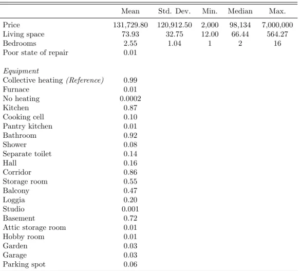
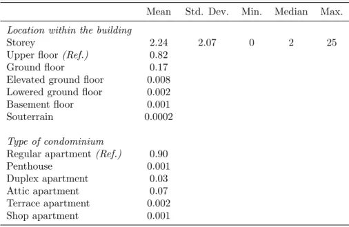
Tables 3 through 7 show the summary statistics for all relevant variables.

On average, a condominium was worth 131,729.80 e or 1,658.48 e per m² taking all transactions in the sample into account. Not surprisingly, most appartments had some cooking spaces, a toilet and a heating system. About half of all transactions have a balcony and a storage room. About 72% have access to a basement (either as owner or separate use privilege). On the contrary, garages and parking lots are very seldom part of a transaction (0.03%

and 0.06% respectively).

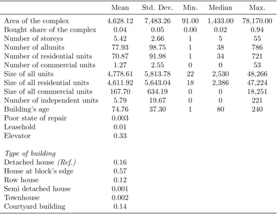
Table 5 reports summary statistics for characteristics of the builing complex the condominium is part of. We have information on the number of commer- cial units within the building and can distinguish between high rise apartment complexes and rather small units. On average, buildings (and hence the con- dominiums) are over 74 years old when they get sold. This corresponds to the construction phase after World War II. The number of sales appears to be relative constant over the years ranging from y.

In total, 106 variables characterize a transaction in the original dataset. Of which, 19 variables are continuous variables. The remaining ones are discrete variables treated as common factor variables in the model. As carried out above in section 2, there are two possible ways of how factor variables can become part

of a model. On the one hand factor variables can enter the regression equation only once (represented by their corresponding dummy variables) or on the other hand, several times as part of interactions with for instance continuous variables like the floor size. In most cases, we generated a lot of new interacted variables for each factor. But for some variables, namely subdistricts and quarter dummies, this would have lead a computationally unfeasible size of the design matrix. r

The location is determined by the condonomium’s address and a set of variables indicating to which block, subdistrict and district it belongs. It is also reported whether the condominium lies in the former West Berlin or East Berlin. The address of each observation is used to obtain lateral and longi- tudinal coordinates in the Soldner system¹⁵. The GAA regularly evaluates the quality of each residential location with regard to the attractiveness for owners and residents (stadtr¨aumliche Wohnlage), ranging from simple to ex- cellent. This information is also provided for each observation. We included all locational information in the final regression models¹⁶. The only exception, as stated above, are the subdistrict dummies which enter the regression equation only once.

The condominia themselves are described by their living area, number of bed- rooms, location within the building and equipment. Also, the data contains information on additional space belonging to the condominium, like a balcony, hobby room, car park or storage space. It is also documented if the condo- minium is in poor state of repair.

The buildings containing the condominia are characterized by the location within their blocks, their year of construction, number of storeys and the number and total space of all residential and nonresidential units. As with the condominia themselves, poor state of repair is also documented.

Further, the data contains information on the legal status of the contracting parties, the type of contract, subsidies and the occupational status of the con- dominium. Some additional variables of purely administrative purpose are also

15See also f¨ur Stadtentwicklung (2015).

16This holds, of course, only for the more elaborate regression model (Ridge, Lass and Elastic Net). We specified a very parsimonious baseline OLS model.

contained in the original dataset, but are of no relevance to the transaction and are therefore ignored.

The date of transaction was used to generate year and quarter dummies yield- ing a total of 90 factors (18 years and 72 quarters). For computational reasons, quarter dummies enter the regression only once (not interacted with other vari- ables).

3.2 Data cleansing

The goal in preparing the dataset for the forthcoming analysis is to lose as little information as possible, while at the same time retaining a computationally feasible level of complexity.

Unlike in other works on similar datasets, no adjustment is made for in- flation or changes in the real estate market¹⁷. Such effects are handled by including detailed information on the time of transaction in the model.

Variables are deleted if they are either of purely administrative nature, if their values were not continuously reported throughout the observed time period, or if they contain excessive amounts of missing values for other unknown reasons.

For computational reasons, dummy variables indicating to which block and subdistrict an observation belongs are discarded, leaving the lateral and longi- tudinal coordinates and dummy variables indicating the district and affiliation to East or West Berlin as variables describing an observation’s location. In addition, the distance to the city center is calculated, with the Pariser Platz serving as Berlin’s center.

To allow log-transformation, several continuous variables need to be slightly adapted: the minimal value for the condominium’s storey, distance to the city center, the bought share of the complex, the number of commercial units within the complex and their total size, and the number of independent aux- iliary units are all set from zero to 0.1.

Regarding spaces detached from a condominium, German law (specifically the Wohnungseigentumsgesetz) differentiates between ownership (Sondereigen-

17See Kolbe et al. (2012), for example, who use house price indixes to convert prices.

tum) and the right of separate use (Sondernutzungsrecht). The original dataset distinguishes between these two legal terms for basements, attics, garages, parking spots and hobby rooms. For this analysis, this distinction is not adopted, but rather it is only stated whether the occupant has exclusive access to such a detached space, regardless of ownership.

Observations are only deleted from the dataset if they are atypical with regard to the contract, clearly misspecified or lack critical information. Thus, forced auctions and transactions where a condominium is only partially sold are removed. So, too, are condominia where the reported average size of bedrooms is less than 8 m², and two cases where the size is unknown, but the reported number of bedrooms are 43 and 67. Transactions for less than 20 e per m² are also deleted, since such a low price can only result from misspecification or substantial irregularities not displayed by the available information. If neither the size, nor the number of bedrooms is known, the observation is deleted.

The same goes for observations where the apartment complex’s area, number of storeys and total living space of the complex are jointly unknown. Most likely due to spelling errors or changes in the street name since the time of transaction, 19 observations are deleted because they cannot be located. Thus, 1672 observations are deleted, resulting in a loss of less than one percent and leaving 186,923 observations.

3.3 Imputation of missing values

Eight variables contain a manageable amount of missing values or values clearly indicating that the information is unknown or misspecified. Deleting all obser- vations with any missing values would contradict the goal of retaining as much information as possible. The easiest approach would consist of filling in the median value of the non-missing values, but in the case of variables describing real estate, it is reasonable to assume that one can do better by exploiting dependencies between the characteristics for filling in the missing values¹⁸. In order to recover the missing information, linear regression imputation is used,

18Hastie et al. (2009) p. 332

with the exception of the building’s age, where missing values are recovered by a sort of nearest neighbour algorithm. The danger with regression imputation lies in artificially driving up the correlation between covariates and underes- timating the variability of the variable containing missing values¹⁹. However, the correlation between the characteristics in question is already very high, and no variable shows more than six percent missing values. Thus, the danger of distortion is acceptable for such a procedure. More elaborate approaches as stochastic regression imputation or multiple imputation²⁰ would have in- creased the already high computational burden of the given research question.

Imputation is rather seen as a necessity, having to be dealt with in a quick and efficient fashion in order to secure the goal of minimal information loss.

Thus, the used regression models are chosen by picking the variables deemed most likely to have high correlation with the dependent variable in question, and no transformations or interactions are included.

On 10,728 occasions the size of all residential units of the building in ques- tion is either missing or reported as smaller than the sold condominium. The area of the apartment complex, the number of residential units and the num- ber of independent auxiliary units serve as predictors to recover the missing values. Where the area is also unknown, a prediction is made by using only the remaining two covariates.

623 occasions of an unknown area of the apartment complex are imputed via the building’s number of storeys, the number of residential units and of inde- pendent auxiliary units.

The number of the building’s storeys is unknown 942 times and is predicted via the area of the complex, the number of residential units and whether or not the building is equipped with an elevator.

The condominium’s living space (250 missing values) and the number of bed- rooms (2,582 missing values) serve as predictors for each other (observations where this information is jointly missing have already been excluded).

The total space of all residential and shared units is reported as smaller than the sold condominium on 10,669 occasions. These missing values are predicted

19van Buuren (2012), p. 12

20See van Buuren (2012), chapters 1.3.5 and 1.4

via the total space of all residential units and the number of residential and shared units.

50 occasions of the number of residential units being reported as zero are im- puted using the total size of all residential units.

The building’s age is unknown for 365 observations. For this particular vari- able, regression imputation is unsuitable, and a neighborhood search is used to impute the missing values. Starting with a radius of 25 meters, all obser- vations within a circle around the observations of interest are identified. The most frequent value of the surrounding buildings’ age is taken as prediction for the missing value. If no observations are within the circle, the radius is widened by an additional 25 meters, until all missing values have been filled in. Although this method can (and on multiple occasions surely does) lead to poor predictions due to the heterogeneity of the Berlin map with regard to the era in which buildings were erect, it is considered more valuable to keep the observation and risk a misspecified building’s age, rather than lose all the observation’s information on the numerous other characteristics.

Different approaches exist to check the validity of the imputation results.

All methods have in common that they compare whether the distribution of the variables before and after recovering the missing values remain compara- ble. Popular methods are graphical checks, numerical summaries or statistical tests²¹. Again, pointing to the fact that this is by no means the focus of this work, the easiest of these methods is used here and numerical summaries are employed for checking the imputation results. As reported in table 8, the range, quartiles and means are hardly affected for all eight variables subject to imputation, suggesting a successful imputation process.

A complete overview of all variables used for further analysis is given in tables 3 through 7. After the mentioned additions and transferring categorical variables into dummies, each transaction is now described by 19 metric vari- ables (including the price) and 81 dummy variables (not including reference categories).

21See Nguyen et al. (2017)

4 Results

As described in subsection (2.7), we performed our prediction comparison in a rolling window design. Table 9 in the Appendix gives details about the size of the estimation and validation samples in each of our 32 prediction windows.

On average, there are about 104,000 observations in an estimation sample and about 2,900 observations in a validation sample. In total, over all windows and validation sample, we have obtained 93,436 prediction errors for each of our four candidate procedures. We first present results from analyzing all these prediction errors together. Subsequently, we also look at results broken down by prediction windows.

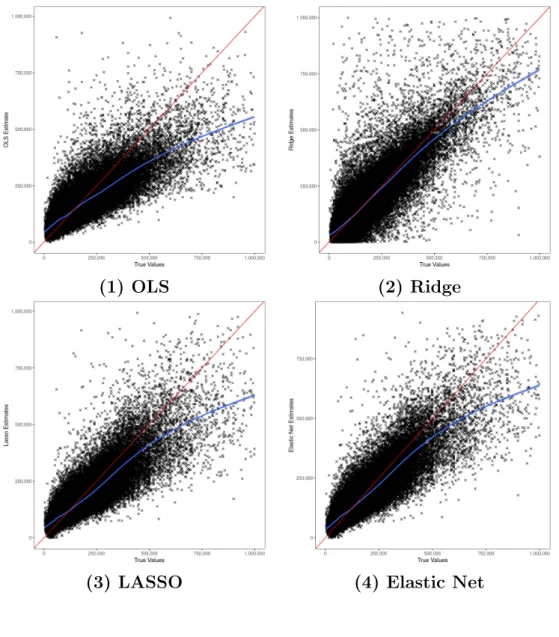
We begin with a graphical analysis of the predictions underlying the predic- tion errors. The scatterplots in Figure 2 show how closely the predicted values of each procedure mimic their targets, the actual sales prices of the properties that were predicted by the AVM methods. Observations where either the ac- tual price or the prediction exceeded 1,000,000eare excluded from the plot to increase readability in the range of prices that include the bulk of the data. In each scatterplot, we have included a 45^◦ line to help in identifying properties that are under- or overvalued by a candidate AVM. We have also included a univariate nonparametric estimate of the relationship between transaction prices and AVM predictions (blue line). Indeed, the comparison of the 45^◦ line and the nonparametric smooth reveals the main finding of this part of the analysis. All models tend to overestimate low priced condominiums while we see a strong tendency to underestimate observations from the right tail of the price distribution. OLS appears to have the strongest tendency underestimate the values of more expensive properties. This is to be expected as it is the least flexible procedure with the greatest risk of a model bias. Ridge regression shows a particularly close agreement (i.e., small bias) between the nonpara- metric smooth and the 45^◦ line for properties up to 500,000 e, whereas the Elastic Net seems to have the overall tightest agreement between nonparamet- ric smooth and 45^◦ line. On the other hand, Ridge regression displays a strong variation about the 45^◦ line, especially for lower priced condominiums.

Figure 2: Scatterplots of true transaction prices vs. model estimates. Note: The blue line is a nonparametric fit, the red line is the 45^◦ line .

(1) OLS (2) Ridge

(3) LASSO (4) Elastic Net

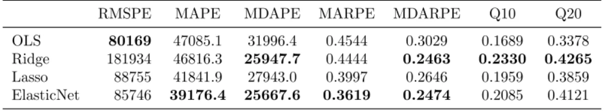
The findings from the inspection of the scatterplots in Figure 2 are largely underscored by the summary measures of the prediction errors reported in Table 1. We have highlighted the result of the best performing procedure in

Table 1: Error metrics for all models aggregated over all forecast quarters.

RMSPE MAPE MDAPE MARPE MDARPE Q10 Q20

OLS 80169 47085.1 31996.4 0.4544 0.3029 0.1689 0.3378 Ridge 181934 46816.3 25947.7 0.4444 0.2463 0.2330 0.4265 Lasso 88755 41841.9 27943.0 0.3997 0.2646 0.1959 0.3859 ElasticNet 85746 39176.4 25667.6 0.3619 0.2474 0.2085 0.4121

bold face for each criterion. Strikingly, OLS, the simplest AVM procedure has the lowest root mean squared prediction error. Apparently, it can compensate for its visible bias in Figure 2 by its very small estimation variance indicated by formula (3) above. Its model bias also shows up in all the mean and median absolute prediction error criteria where it always performs worst. Also as expected from Figure 2, the Elastic Net performs best with regard to all bias criteria and outperforms Lasso, the procedure it generalizes, with regard to all criteria. A particularly uneven performance is offered by Ridge regression. It displays the best performance with regard to the Q₁0 and Q₂0 criteria. That is, Ridge regression achieves the largest fraction of predictions within 10 or 20 percent of the actual sales price. However, it is by far the worst procedure in terms of the root mean squared prediction error. Apparently, it performs really well for ‘standard’ properties in the center of the distribution but extremely poorly for some properties at the fringe.

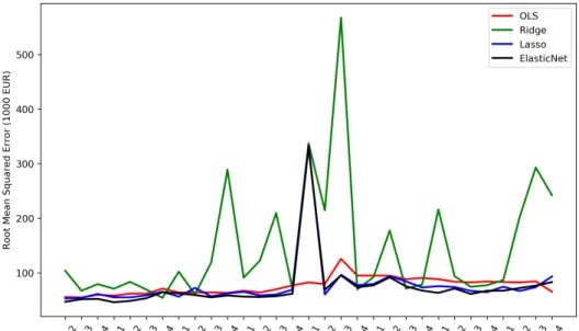
Indeed, this becomes even more evident in figure 3 which plots the RMSPE for each procedure over the course of the rolling window design. The RMSPE values for Ridge regression (connected by a line to enhance readability) show very large bumps for some evaluation periods²². In these periods, there were some properties for which Ridge regression delivered extremely false predic- tions. These errors are highlighted by RMSPE because of the built-in squaring

22We see a similar bump in one quarter also for the Elastic Net.

Figure 3: Root mean squared error for every validation quarter of the rolling window design

of prediction errors. Ridge regression shrinks coefficients but does not set them to zero. Its prediction formula thus carries a large number of nonzero param- eters, thereby increasing the risk for such a bad outcome if properties display extreme values in the transformed feature space.

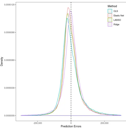
The uneven prediction performance of the Ridge regression AVM is also visible in Figure 4. It shows kernel densities of the prediction errors of all four models.²³ We have restricted the range of the prediction errors to the interval

−300,000 to 300,000. The extreme errors of Ridge regression are deliberately not shown as they would dwarf any differences that may exist within the bulk of the errors. The low median absolute errors of Ridge are reflected by its density being almost centered at zero (stemming from its high flexibility). Its large fractions of Q10 or Q20 are visible in its density being relatively tightly and symmetrically centered around the median. Indeed, from the perspective of Figure 4, which omits its extremely poor performance at the fringes, Ridge regression looks like a winner. All procedures, except for OLS, start with a

23We used the Epanechnikov kernel and calculated the bandwidth according to the pro- posal by Venables and Ripley (2002).

Figure 4: Density plots of prediction errors of all models across all prediction quarters.

large number of parameters and then either shrink some of them or even set some of them to zero. Indeed, with their ability to do the latter, the Lasso and the Elastic Net offer the promise of ‘automatic’ variable selection. We explore the patterns of shrinkage and variable exclusion achieved by these procedures in Figures 5, 6 and 7. These plots are based on summing the estimated coefficients of each transformed feature z_m for the respective model across all prediction periods. In the plots, we ordered them by size. Hence, features are visible that often (i.e. in several prediction windows) ‘survive’ the shrinkage or selection algorithms of the procedures. We normalized the vertical axes of the figures by substracting the minimum and divididing by the difference between maximum

and minimum over all coefficient sums. Our feature importance measure is thus exactly one at the maximum. As all variables were normalized prior to estimation, the size of their coefficients are comparable. The figures show that across all procedures, the squared floor size is the strongest predictor in this sense. Indeed, floor size appears ‘successful’ in various (interacted) forms and emerges as the most robust determinant in these AVMs.

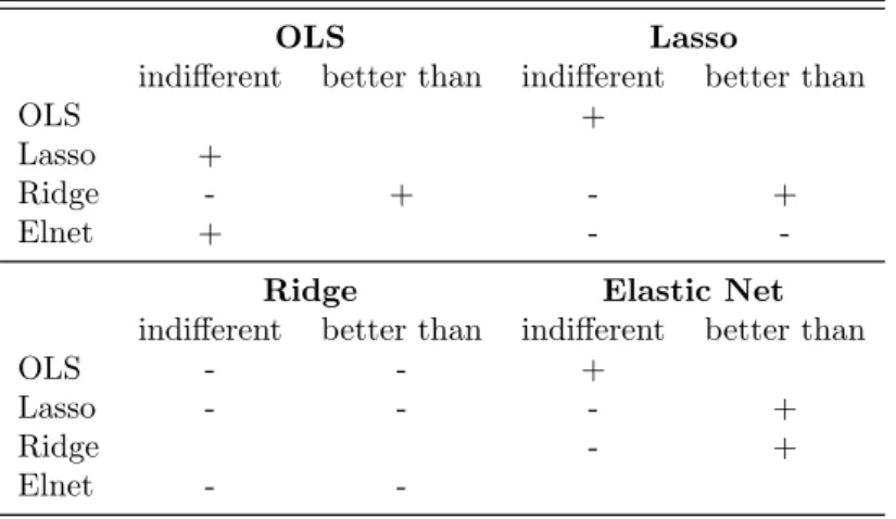
Lastly, we performed an adjusted Diebold-Mariano-Test as described at the end of subsection 2.7. In a first run, we tested whether there is a significant difference between the prediction performance of any two models. In a second step, we performed a one-sided test which evaluated if one model has a signif- icantly better performance than the other. After comparing each model with every other model, it turns out that except for Ridge every other model has no significant better forecast performance than OLS. Elastic Net performs better than the Lasso estimator. Table 2 reports the test results a “+” indicates that the null hypothesis can not be rejected and “-” if the hypothesis was rejected.

If the two sided test found no significant difference between two models (“+”), the second test is discarded. These findings are in line with the error metrics.

We use a squared loss function for testing the hypotheses and as OLS produces the smallest squared prediction errors the results are not surprising.

Table 2: Results of the Diebold-Mariano Tests. A ‘-’ indicates that the Null hypotheses was rejected on a 5% significance level.

OLS Lasso

indifferent better than indifferent better than

OLS +

Lasso +

Ridge - + - +

Elnet + - -

Ridge Elastic Net

indifferent better than indifferent better than

OLS - - +

Lasso - - - +

Ridge - +

Elnet - -