Oceanic lithospheric S -wave velocities from the analysis of P -wave polarization at the ocean floor

(1)

Geophysical Journal International

Geophys. J. Int.(2016)207,1796–1817 doi: 10.1093/gji/ggw342

Advance Access publication 2016 September 14 GJI Seismology

Oceanic lithospheric S -wave velocities from the analysis of P -wave polarization at the ocean floor

Katrin Hannemann,

¹

Frank Kr¨uger,

²

Torsten Dahm

^2,3

and Dietrich Lange

¹

1GEOMAR, Helmholtz Centre for Ocean Research Kiel, Kiel, Germany. E-mail:khannemann@geomar.de

2Institute of Earth and Environmental Science, University of Potsdam, Potsdam-Golm, Germany

3Section2.1, Physics of Earthquakes and Volcanoes, GFZ Potsdam, Potsdam, Germany

Accepted 2016 September 14. Received 2016 August 29; in original form 2016 March 22; Editorial Decision 2016 September 12

S U M M A R Y

Our knowledge of the absoluteS-wave velocities of the oceanic lithosphere is mainly based on global surface wave tomography, local active seismic or compliance measurements using oceanic infragravity waves. The results of tomography give a rather smooth picture of the actualS-wave velocity structure and local measurements have limitations regarding the range of elastic parameters or the geometry of the measurement. Here, we use theP-wave polarization (apparent P-wave incidence angle) of teleseismic events to investigate the S-wave velocity structure of the oceanic crust and the upper tens of kilometres of the mantle beneath single stations. In this study, we present an up to our knowledge new relation of the apparent P- wave incidence angle at the ocean bottom dependent on the half-spaceS-wave velocity. We analyse the angle in different period ranges at ocean bottom stations (OBSs) to derive apparent S-wave velocity profiles. These profiles are dependent on theS-wave velocity as well as on the thickness of the layers in the subsurface. Consequently, their interpretation results in a set of equally valid models. We analyse the apparentP-wave incidence angles of an OBS data set which was collected in the Eastern Mid Atlantic. We are able to determine reasonable S-wave-velocity-depth models by a three-step quantitative modelling after a manual data quality control, although layer resonance sometimes influences the estimated apparentS-wave velocities. The apparent S-wave velocity profiles are well explained by an oceanic PREM model in which the upper part is replaced by four layers consisting of a water column, a sediment, a crust and a layer representing the uppermost mantle. The obtained sediment has a thickness between 0.3 and 0.9 km withS-wave velocities between 0.7 and 1.4 km s⁻¹. The estimated total crustal thickness varies between 4 and 10 km withS-wave velocities between 3.5 and 4.3 km s⁻¹. We find a slight increase of the total crustal thickness from∼5 to∼8 km towards the South in the direction of a major plate boundary, the Gloria Fault. The observed crustal thickening can be related with the known dominant compression in the vicinity of the fault. Furthermore, the resulting mantle S-wave velocities decrease from values around 5.5 to 4.5 km s⁻¹ towards the fault. This decrease is probably caused by serpentinization and indicates that the oceanic transform fault affects a broad region in the uppermost mantle.

Conclusively, the presented method is useful for the estimation of the localS-wave velocity structure beneath ocean bottom seismic stations. It is easy to implement and consists of two main steps: (1) measurement of apparentP-wave incidence angles in different period ranges for real and synthetic data, and (2) comparison of the determined apparentS-wave velocities for real and synthetic data to estimateS-wave velocity-depth models.

Key words: Time-series analysis; Body waves; Theoretical seismology; Oceanic transform and fracture zone processes.

1 I N T R O D U C T I O N

The polarization angle of the particle motion (apparent incidence angleϕp) of an incomingP(compressional) wave at the free surface

or the solid-liquid interface is the result of a superposition of the displacements of the incidentPwave and the reflectedPwave andS (shear) wave. The measured polarization of thePwave (i.e. apparent P-wave incidence angleϕp) therefore differs from the real incidence 1796 ^CThe Authors 2016. Published by Oxford University Press on behalf of The Royal Astronomical Society.

at GEOMAR Helmholtz-Zentrum fuer Ozeanforschung Kiel on November 23, 2016http://gji.oxfordjournals.org/Downloaded from

(2)

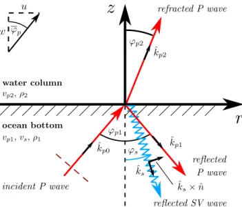
angleϕp1of the incidentPwave (Fig.1). Wiechert (1907) showed that for the case of the free surface, the apparentP-wave incidence angle ϕp is twice the angle of the reflected SVwave (vertically polarizedSwave,ϕs). The analytical determination of the apparent P-wave incidence angleϕp is based on the reflection coefficients at the corresponding interface (i.e. free surface or ocean bottom).

Due to the influence of the water column (WC), the relation of the apparentP-wave incidence angle valid for the ocean bottom has to differ from the free surface relation given by Wiechert (1907).

The apparent incidence angle can be interpreted in different ways.

Measurements of the apparentP-wave andS-wave incidence angles were used by Nuttli & Whitmore (1961,1962) to determineP-wave velocities from P-waves with periods of 3–7 s andSwaves with periods in the order of 10 s. They foundP-wave velocities over 7 km s⁻¹. This result was interpreted by Phinney (1964) to be an indicator that the polarization is dependent on the period range used for the analysis and that for shorter periods lower velocities would be obtained. Kr¨uger (1994) used theP-wave polarization to study the sedimentary structure at the Gr¨afenberg array in southern Germany by analysing the steepening of the P wave onset in terms of the ratio between P-wave andS-wave velocities. Whereas Svenningsen &

Jacobsen (2007) and Kielinget al.(2011) used a progressive low- pass filtering of receiver functions (RFs) and the relation presented by Wiechert (1907) to perform an inversion for anS-wave velocity- depth model.

Usually, theP-wave polarization angle is determined by the measurement of the particle motion on the vertical (Z) and radial (R) component of a seismogram (Kr¨uger 1994). This measurement needs a careful time window selection and data preparation, because it is influenced by the often complicatedP-wave signal. Svenningsen

& Jacobsen (2007) proposed to use (Z, R) RFs instead of the raw earthquake signal to avoid this complexity issue and to ease auto- matic processing. The earthquake signal is deconvolved either in time domain (Kindet al.1995; Kielinget al.2011) or frequency domain (Ammon1991). This procedure transforms theP-wave signal into a (band limited) spike like signal on the vertical and radial component of the RF att=0. Thus, the apparentP-wave incidence angle can be measured by determining the amplitudes of the spike on the two components (Svenningsen & Jacobsen2007).

Ocean bottom stations (OBSs) are sensors constructed for the deployment on the ocean floor (Webb 1998; Dahmet al.2006).

Often, OBS recordings have a poor signal-to-noise ratio (SNR) and suffer from high noise levels especially on the horizontal components. This results in a small number of usable event recordings for these sensors which usually operate for one year or less (Webb 1998). We increase the number of usable recordings by including Pdiff(90^◦–110^◦epicentral distance) and PKP (140^◦–160^◦) recordings besidesP-wave recordings (30–90^◦) in our analysis. Further- more, we have to reconsider the apparentP-wave incidence angle relation for the free surface presented by Wiechert (1907) for the case of the ocean bottom, because the refracted P wave in the WC has an influence on the reflection coefficients of the ocean bottom.

These coefficients are needed to calculate the displacements within the ocean bottom. The coefficients for the reflection and refraction at the interface between a solid and a liquid half-space were calculated for specific model parameters by Knott (1899). Zoeppritz (1919) presented an analytical calculation of the coefficients which can also be found in some textbooks (e.g. Ben-Menahem &

Singh 1981). These Zoeppritz equations are also used in reflection seismic (e.g. Wang1999b) or RF studies (Juli`a2007; Kumar et al.2014; Kumar2015) to analyse impedance contrasts at inter- faces.

We use the reflection coefficients to obtain a new relation which enables us to determine apparent (half-space) S-wave velocities fromP-wave polarization (apparentP-wave incidence angle) measurements. We employ this relation together with a progressive low-pass filtering analogue to Svenningsen & Jacobsen (2007) and a quantitative modelling to obtainS-wave velocity-depth models.

1.1 Previous studies of oceanicS-wave velocity

TheS-wave velocity structure of the oceanic crust and the upper mantle has mainly been studied by global tomography of surface waves (Romanowicz2003; Laskeet al.2013) using land stations.

The results of those global studies are biased by the poor data cov- erage in the oceans (Romanowicz2003). Moreover, these studies employ long wavelengths for their investigation and the resolution of the gained models is therefore rather low (up to several degrees, Romanowicz2003; Laskeet al.2013). If phase velocities or group velocities are used to determineS-wave velocity maps, several stations or arrays are needed and the obtained results reflect more the average velocity between pairs of stations than single station’s estimates (Weidle & Maupin2008; Maupin2011; Gao & Shen2015).

Another approach to estimate theS-wave velocity structure of the oceanic lithosphere is the seafloor compliance inversion (Yamamoto

& Torii1986; Crawfordet al.1998; Webb1998). This technique analyses the ratio of seafloor displacement to pressure loading due to infragravity waves in a very low frequency band (0.003 to 0.04 Hz, Crawfordet al.1998). The usage of this technique is limited, because the displacement by ocean surface waves at deep water sites is small and difficult to measure (Crawfordet al.1998; Webb1998).

There have also been attempts to extract information about the shallowS-wave velocity structure from active seismic data (e.g. up to 300 m in Ritzwoller & Levshin (2002) and for the upper tens of metres in Nguyenet al.(2009)). The success of these techniques is directly related to the distance of the active source to the seafloor.

The closer the source is located to the seafloor the more acoustic energy can be converted intoS-wave energy (Ritzwoller & Levshin 2002). The inversion of these active data results in high resolution S-wave velocity models, but it is limited to the upper hundreds of metres beneath the seafloor. We therefore propose that by using progressive low-pass filtering (∼0.05 to 2 Hz), the analysis ofP- wave polarization in terms ofS-wave velocities will provide the opportunity to resolve deeper (crustal)S-wave velocity structures than active seismics and will give a better resolution of the crustal S-wave velocity structures than compliance measurements.

First, we use the reflection coefficients provided by Zoeppritz (1919) and Ben-Menahem & Singh (1981) to find a relation for the apparent P wave incidence angle at the ocean bottom analogue to the one presented by Wiechert (1907). Then, we describe the analysis of theP-wave polarization by progressive low-pass filtering of (Z, R) RF and the estimation of apparentS-wave velocities. We perform several synthetic tests to investigate the resolution of the proposed method. Finally, we apply the method to real OBS data from the Eastern Mid Atlantic Ocean and perform a quantitative modelling to determine sedimentary, crustal and mantleS-wave velocities and the thickness of the sediments and the oceanic crust.

2 T H E O RY

Considering a seismometer which measures the displacement on the seafloor, we define a local coordinate system with a verticalz-axis pointing upward and a horizontalr-axis pointing in the horizontal

(3)

Figure 1.Polarities ofP-waves (red) andSVwave (blue) at the interface between water column and ocean bottom. The incomingP-wave front is represented as dashed red line. The particle motions of the single wave types are shown as small black arrows. The normal of thezr-plane ˆnpoints into the negative transverse direction. The ocean bottom has theP-wave velocityv^p1, theS-wave velocityv^sand the densityρ¹. The water column has theP-wave velocityvp2and the densityρ2. The displacementsuandw are measured at the seafloor to estimate theP-wave polarization (apparent incidence angle,ϕp).

propagation direction of the wave front (Fig.1, dashed red line).

Thez-axis is thus parallel to the vertical (Z) component of the recorded seismogram and the r-axis is parallel to the radial (R) component. The displacementuis measured along ther-axis and the displacementwalong thez-axis (Fig.1). The tangent of the ratio of those displacements is used to estimate theP-wave polarization ϕp(apparent incidence angle, Fig.1and Wiechert1907):

tanϕp= u

w. (1)

The displacementsuandwresult from the superposition of the displacements of different elastic waves at the interface between WC and ocean bottom (z=0 in Fig.1). The boundary conditions for the displacement at the interface between a fluid with low vis- cosity, for example, water and a solid are that the displacement normal to the interface (i.e.w) must be continuous, whereas the tangential components (i.e.u) can be discontinuous (Knott1899;

Ben-Menahem & Singh1981; Aki & Richards2002). Assuming the seismometer of an OBS measures the displacement of the ocean bottom, we have to consider the amplitudes of the elastic waves in the ocean bottom to obtain theP-wave polarizationϕpat the ocean floor.

In Fig.1, the unit vectors describing the polarization direction of the incidentP-wave (ˆk_p0), the reflectedP-wave (ˆk_p1) and the reflectedS-wave (ˆk_s×n) are presented.ˆ

kˆ_p0=

⎛

⎜⎝ sinϕp1

0 cosϕp1

⎞

⎟⎠kˆ_p1=

⎛

⎜⎝ sinϕp1

0

−cosϕp1

⎞

⎟⎠kˆ_s×nˆ =

⎛

⎜⎝ cosϕs

0 sinϕs

⎞

⎟⎠,

(2) whereϕp1 andϕs are the angles of the incident (and reflected)P wave, and the reflectedSVwave, respectively and ˆn denotes the normal of thezr-plane. The reflection coefficient ´PP` is defined

as the amplitude ratio of the reflected P wave and the incident Pwave and the reflection coefficient ´PS` is the amplitude ratio of the reflectedSVwave and the incidentPwave. Following Aki &

Richards (2002), we use an acute accent (e.g. ´P) to represent an upcoming wave and a grave accent (e.g. `P) to denote a down-going wave. Considering the reflection coefficients and eq. (2), eq. (1) can be written as:

tanϕp = (1+P´P) sin` ϕp1+P´S`cosϕs

(1−P´P) cos` ϕp1+P´S`sinϕs

. (3)

The numerator and the denominator of eq. (3) are analogue to the displacements inrandzdirections provided by Pilant (1979) and Aki & Richards (2002) for the solid-solid case, and by Ben- Menahem & Singh (1981) for the solid-liquid case. The signs of cosϕp1and cosϕsare negative in Pilant (1979) and Ben-Menahem

& Singh (1981) in which thezaxis is defined downward instead of upward as in the seismometer based definition used here (Fig.1).

We calculated the coefficients ´PP` and ´PS` and compared them to the coefficients published by Zoeppritz (1919):

P´P` = 1− f(1−g)

1+ f(1+g) (4)

P´S` = 4_v^v^s^ρ¹

p2ρ2sinϕp1cosϕp2cos (2ϕs)

1+ f(1+g) (5)

with: f = vp1ρ1

vp2ρ2

cosϕp2cos²(2ϕs) cosϕp1

(6)

g= vs

vp1 2sin

2ϕp1

tan (2ϕs)

cos (2ϕs) . (7)

They are similar besides that Zoeppritz (1919) provides eq. (4) with a negative sign, because his definition of the polarization direction of the reflectedPwave (ˆkp1) is opposite to the definition used here (positive inrand negative inzdirection, Fig.1). In eqs (4)–(7),vp1,vsandρ1are theP-wave andS-wave velocity as well as the density of the ocean bottom, andvp2andρ2are theP-wave velocity and the density of the WC. The coefficients in eqs (4) and (5) are equivalent to the coefficients provided by Ben-Menahem &

Singh (1981) for the mantle-core reflection except for the polarity of ´PS` which can be explained by the before mentioned differing definition of thezaxis.

We insert eqs (4)–(7) in eq. (3) and use Snell’s law sinϕp1

vp1

= sinϕp2

vp2

= sinϕs

vs

= p. . .horizontal slowness (8) to obtain the relation for the apparentP-wave incidence angle at the ocean bottom (see supplementary material for details of calculation):

tanϕp =tan (2ϕs)+ρ2

ρ1

tanϕp2

cos (2ϕs). (9)

The new eq. (9) has two terms, the first term equals the well- known relation for the free surface of a solid half-space (Wiechert 1907) and the second term describes the influence of the WC on the apparentP-wave incidence angle.

(4)

Figure 2. Comparison of eq. (9) and Wiechert formula (ϕp=2ϕs ). The theoretical apparentP-wave incidence angleϕpon the ocean floor if theP- wave incidence angleϕp1is given are shown as solid lines. Theϕpat the free surface ifϕp1is given are shown as dashed lines. The values for an oceanic crust (OC: water layer/ crust, FC: free-surface/ crust, Table1) are shown in blue and the values for a sediment (OS: water layer/ sediment, FS: free- surface/ sediment, Table1) in red. The measured apparentP-wave incidence angles from synthetic seismograms (QSEIS) are presented as circles for the OC model (blue) and the OS model (red).

Using Snell’s law (eq. 8), eq. (9) is re-written as function of the horizontal slowness p(see supplementary material for details of calculation):

tanϕp= p

ρ2 v²s +2ρ1

1

v²s −p² ₁

v²_p2−p² ρ1

1 v²_p2−p²

1 vs²−2p²

. (10)

Eq. (10) shows that the apparentP-wave incidence angleϕp is independent of the P-wave velocity vp1 of the ocean bottom. In Fig.2, we present a comparison betweenϕpfor the ocean bottom and the free surface. It becomes clear that the apparent P-wave incidence angles differ especially for the water/sediment contrast.

Moreover, if apparentS-wave velocities are estimated at the ocean bottom using the free surface relation, the obtained velocities will be higher than the true values (compare eq. 10).

3 M E T H O D O L O G Y

The estimation of apparentP-wave incidence angles (ϕp) can be done by using hodographs of theP-wave particle motion (Kr¨uger 1994). The P-wave train can be rather complex because of the influence of the source time function and the source-to-receiver wave propagation. The analysis of the particle motion therefore requires a careful data preparation and time window selection. The processing is eased by employing RFs for which the R component is deconvolved with the Z component (Svenningsen & Jacobsen 2007). By this procedure, theP-wave signal turns into a zero-phase (band-limited) spike which arrives at timet=0 on the vertical (ZRF) and radial (RRF) component. We perform the deconvolution in time domain by using a Wiener filter (Kindet al.1995; Kielinget al.

2011). The apparentP-wave incidence angle can be estimated by measuring the amplitudes att=0 on ZRFand RRF(Svenningsen &

Jacobsen2007). On RRF, additionally a series ofPtoSconverted signals become visible after the projection of the direct P spike signal.

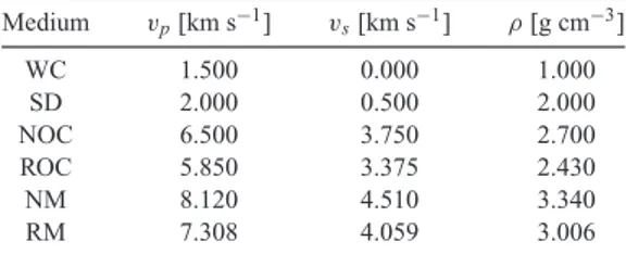
Table 1. Model parameters for standard values of water column (WC), sediment (SD), normal oceanic crust (NOC), oceanic crust with 10 per cent reduced velocities and density (ROC), normal mantle (NM) and mantle with 10 per cent reduced velocities and density (RM). We give theP-wave velocityvp, theS-wave velocityvsand the densityρ. Medium vp[km s⁻¹] vs[km s⁻¹] ρ[g cm⁻³]

WC 1.500 0.000 1.000

SD 2.000 0.500 2.000

NOC 6.500 3.750 2.700

ROC 5.850 3.375 2.430

NM 8.120 4.510 3.340

RM 7.308 4.059 3.006

The seismic velocities obtained by analysing theP-wave polarization (apparentP-wave incidence angle,ϕp) are dependent on the used period range (Haskell1962; Phinney1964). For longer periods (∼5–10 s), the obtained velocities are typical for the Earth’s mantle (Nuttli & Whitmore1961,1962). If shorter periods are used for the measurement of theP-wave polarizationϕp, the estimated velocities will be similar to crustal velocities (Phinney1964; Sven- ningsen & Jacobsen2007). This behaviour can be used to obtain velocity-depth profiles (Svenningsen & Jacobsen2007). In order to analyse the apparentP-wave incidence angles, we apply a set of different low pass filters to the (Z, R) RF before estimating the angles (Svenningsen & Jacobsen2007). We use Butterworth low-pass filters of second order which are applied forwards and backwards in order to get zero phase filters (Scherbaum2001). The corner periods of the filters are chosen to be logarithmically distributed as suggested by Svenningsen & Jacobsen (2007).

The (Z, R) RFs are calculated and filtered withLlow pass filters forN events. After the filtering, the apparent P-wave incidence anglesϕ^obsp,n(T_l) are measured for each corner periodT_lat timet=0 of the filtered (Z, R) RFs. A misfit functionmcan be formed which compares the measured apparentP-wave incidence anglesϕ^obsp,n(Tl) forNdifferent events with their calculated theoretical equivalent ϕ^theop using eq. (10) for each corner periodTl:

m(vs, ρ1,Tl)= 1 N n=1

wn

· N n=1

(|D(T_l, vs, ρ1,pn)| ·wn) (11)

with

D(Tl, vs, ρ1,pn)=tanϕ^obsp,n(Tl)−tanϕ^theop (vs, ρ1,pn).

The weightswnare chosen based on data quality. Standard values (Table1) are used for theP-wave velocityvp2and densityρ2of the WC to calculate the theoretical angleϕ^theop (eq. 10). The horizontal slownesspnfor each eventnis calculated for global velocity models (AK135, Kennettet al.1995). The remaining unknowns in eq. (11) are theS-wave velocityvsand the densityρ1of the ocean bottom.

In the following section, we perform synthetic tests to analyse the dependency of the apparent incidence angle on theS-wave velocity vsand the densityρ1, as well as its behaviour in dependence on the used corner periodTlfor multilayered models.

4 S Y N T H E T I C T E S T S

In this section, we want to investigate typical structures of the ocean bottom by calculating synthetic data for different oceanic layered velocity models with a full wave field reflectivity method (QSEIS;

(5)

Table 2. Model description for synthetic tests (regional case). All models include a water column (WC) of 5.05 km (layer 1). Layer thickness for sediment (SD), normal oceanic crust (NOC) and normal mantle (NM) (for model parameters, see Table1). The source depth is given in kilometres b.s.f.

Model Layer 2 Half-space Source depth [km b.s.f.]

OC – NOC 100

OS – SD 100

N 7 km NOC NM 100

S100C 0.1 km SD NOC 100

S200C 0.2 km SD NOC 100

S300C 0.3 km SD NOC 100

S400C 0.4 km SD NOC 100

S600C 0.6 km SD NOC 100

S800C 0.8 km SD NOC 100

S1000C 1 km SD NOC 100

Table 3. Description of models at the receiver site for synthetic tests (teleseismic case). All models include a water column (WC) of 5.05 km (layer 1), PREM below 155.05 km and continental PREM for the source site (Support- ing Information Fig. S1). Layer thickness for normal oceanic crust (NOC), oceanic crust with 10 per cent reduced velocities and density (ROC), normal mantle (NM) and mantle with 10 per cent reduced velocities and density (RM) (for model parameters, see Table1).

Model Layer 2 Layer 3 Layer 4 Layer 5

CM-REF 7 km NOC 143 km NM – –

CI 1 km ROC 6 km NOC 143 km NM –

CII 3 km NOC 1 km ROC 3 km NOC 143 km NM

CIII 6 km NOC 1 km ROC 143 km NM –

MI-50 7 km NOC 50 km RM 93 km NM –

MII-50 7 km NOC 3 km NM 50 km RM 90 km NM

MIII-50 7 km NOC 13 km NM 50 km RM 80 km NM

MIV-50 7 km NOC 23 km NM 50 km RM 70 km NM

MV-50 7 km NOC 43 km NM 50 km RM 50 km NM

MVI-50 7 km NOC 93 km NM 50 km RM –

Wang1999a) using the model parameters listed in Table1. We use a normalized squared half-sinus function with a length of 0.5 s which has a flat spectra below 2 Hz as source time function. The reflectivity method is not able to model a liquid layer with anS-wave velocity vs=0 km s⁻¹, instead we use a very soft solid layer for which the P- toS-wave velocity ratio is 1000 as suggested by M¨uller (1985).

The sensor depth is chosen to be 1 m below seafloor (b.s.f.).

In order to save computation time and to obtain high-frequency synthetic data, we first simulate deep regional events (100 km depth) instead of teleseismic global events. The models for the regional case are listed in Table2. In a first step, we test the accuracy of QSEIS against the theoretical expression in eq. (10) using two half- space models. Afterwards, we add one layer to investigate the depth resolution of the proposed method. In a third step, we simulate teleseismic global events with a low sampling frequency (8 Hz) to investigate the influence of water depth and a low velocity layer (LVL; Table3). For the synthetic tests in this section, we set all weights (wnin eq. 11) to one.

4.1 Half-spaceS-wave velocity

The first deep regional source models (model OC and OS, Table2) consist of one layer over a half-space. Model OC includes a WC (Table1) and a normal oceanic crust (NOC, Table1) half-space, and model OS a WC and a sediment (SD, Table1) half-space. An explosion source is located at 100 km b.s.f. and the receivers are placed in 5 to 100 km epicentral distance with 5 km inter-station spacing. This setting corresponds to slowness values of 0.9 s/^◦ to 12.1 s/^◦for the OC model and 2.8 s/^◦to 39.3 s/^◦for the OS model, respectively. The sampling rate is 100 Hz.

The apparentP-wave incidence angles ϕ^obsp,n are determined by measuring the polarization for the P wave of each synthetic event within a 1 s time window for unfiltered data on the Z and R components (circles in Fig.2). By directly comparing, we find a good agreement between measured and theoretical angles for the OC model (solid blue line and blue circles in Fig.2) and the OS model (solid red line and red circles in Fig.2). This shows that the apparent P-wave incidence angles obtained from synthetic data (QSEIS) are similar to the values estimated with our theoretical expression in eq. (10).

Furthermore, we test the dependency of the misfit m(vs, ρ1) (eq. 11) on theS-wave velocityvsand the densityρ1by using the measured apparentP-wave incidence angles of the OC model.

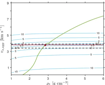
The misfit is calculated based on a grid search overS-wave velocityvs(0.1–9.0 km s⁻¹in 0.1 km s⁻¹steps) and densityρ1(1.0- 6.0 g cm⁻³in 0.1 g cm⁻³steps). The result shows that the dependency of the misfit functionm(vs,ρ1) and therefore of the apparent P-wave incidence angle on theS-wave velocityvsis much stronger than on the densityρ1 (Fig.3). By searching for the minimum in the misfit for each tested density valueρ1, anS-wave velocity range (black dashed lines in Fig.3) is determined, for which a median (red line in Fig.3) is estimated. In the presented case, the median of the apparentS-wave velocityvs,appis 3.8 km s⁻¹and its range is 3.4–3.9 km s⁻¹. If we do not put any constrains on the density for a grid search with aS-wave velocity step size of 0.1 km s⁻¹, the

Figure 3.Misfit functionm(vs,ρ1) calculated by eq. (11) is shown as blue contours overS-wave velocityvsand densityρ1of the ocean bottom for the OC model with WC over NOC. The range in the apparentS-wave velocity vs,app estimated by the minimum of the misfit for each tested density is indicated by black dashed lines. The median of the apparentS-wave velocity v^s,appfor all tested densities is shown in red. The relationρ¹(v^s) is presented in green and the estimatedv^s,appfor the root search is depicted as red circle.

(6)

obtained medianvs,app=3.8 km s⁻¹is a good estimate of theS-wave velocity used in the model (vs=3.75 km s⁻¹).

Instead of a grid search, we can perform a root search to estimate vs,appby assuming a relation between the densityρ1and theS-wave velocity vs. There are well known empirically derived relations between the densityρxand theP-wave velocityvpx(Brocher2005, eq. 12), forvpxin km s⁻¹andρxin g cm⁻³).

ρx =1.6612·vpx−0.4721·v²px+0.0671·v³px

−0.0043·v⁴_px+0.000106·v⁵_px. (12) To obtainρ1(vs), we have to assumevp(vs). ForS-wave velocities up to 2.5 km s⁻¹, the mud-rock line (vp=1.16·vs+1.36, Castagna et al.1985) serves quite well. For largerS-wave velocities, a constant vp/vs ratio could be assumed (vp/vs =√

3 for 2.5 km s⁻¹ < vs

≤ 4.0 km s⁻¹ and vp/vs = 1.8 forvs > 4.0 km s⁻¹). By using the assumed relationρ1(vs) (green line in Fig.3) in eq. (11), the minimum misfitm(vs,ρ1(vs)) for the OC model is estimated atvs,app

=3.76 km s⁻¹(red circle in Fig.3) for anS-wave velocity step size of 0.005 km s⁻¹. This velocity is in good agreement with the used model parameter (vs=3.75 km s⁻¹) and similar to the medianvs,app

obtained by the grid search with a coarser step size.

In conclusion, the weak dependency of the misfit functionm(vs, ρ1) (i.e. the apparentP-wave incidence angle) on the density shows that we could hardly resolve densities with the presented method.

We therefore will neglect the weak influence of the density in the further processing.

In the next section, we analyse the behaviour ofvs,appwith the periodTlfor a layered model and compare the results obtained by estimating the medianvs,appwith the grid search and by determining

vs,app using the root search. Both approaches have proved to give

good estimates of the true half-spaceS-wave velocity.

4.2 Depth resolution

We use several synthetic models to test the depth resolution of the method. All models presented in Figs4and5include a 5.05 km thick WC which is given by CRUST 1.0 for the area of the OBS deployment (Supporting Information Fig. S1; Laskeet al.2013). The angles in Table4give the direction the ray travels within the half- space and are measured towards the normal of the layer interface (i.e. against vertical). The associated slowness values are also given in Table4. The vertical component of the synthetic data (100 Hz) is used to create a Wiener filter, choosing a 5 s time window starting at thePonset. The filter is used to deconvolve the vertical and radial components in order to estimate (Z, R) RF for the analysis. The RF are filtered with a set of low pass filters withLcorner periods Tlwhich are logarithmically distributed (0.5 s to 64 s, 8 filters per octave). The apparentP-wave incidence angles are estimated from the amplitudes on ZRFand RRFat timet=0 (relative to deconvolved Pspike on ZRF).

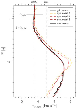
We test model N which consists of 7 km NOC (Table1) over a normal mantle (NM, Table 1) half-space b.s.f. We obtainm(vs, ρ1, Tl) andm(vs, ρ1(vs), Tl) for the estimated apparent P-wave incidence angles and different periods Tl. The minima of misfit m(vs, ρ1,Tl) are determined for each densityρ1. We obtain the medianvs,app for each periodTl and estimate the roots of m(vs, ρ1(vs),Tl) to get the vs,app profiles (black and grey solid line in Fig.4). To show the variability of the results for slowness values typical for P and Pdiff(4–9 s/^◦,∼30^◦–110^◦epicentral distance) and PKP_df(1–2 s/^◦,∼140^◦–160^◦epicentral distance), we included the medianvs,appprofiles for synthetic event 1 (1.19 s/^◦, dashed yellow

Figure 4.Synthetic test for model N (7 km NOC over NM half-space below seafloor, Tables1and2). TheS-wave velocities used in the model are marked by dashed light grey lines. The medianvs,appprofiles obtained for synthetic event 1 (dashed yellow, Table4), synthetic event 4 (dash-dot red, Table4) and synthetic event 8 (dashed red, Table4) are shown. The medianvs,app

profile obtained from the total misfit function of all events (grid search, eq. 11) is shown in black. Thevs,appprofile estimated using the root search is presented in grey.

Figure 5.Synthetic tests for two layers (including WC and SD) over NOC half-space. Detailed model description can be found in Table2and used parameters in Table1. Left panel shows used velocity models for depth below seafloor (b.s.f.). Right panel shows estimatedvs,app profiles with corner periodT.

line in Fig.4), synthetic event 4 (4.68 s/^◦, dash-dot red line in Fig.4) and synthetic event 8 (8.80 s/^◦, dashed red line in Fig.4).

Thevs,appprofiles obtained by the grid search and the root search agree very well. The only difference is the smoother appearance of the root search profile due to the smaller step size invs(0.005 km s⁻¹ compared to 0.1 km s⁻¹). Besides this, the overall appearance of both profiles is identical.

(7)

Table 4. Take-off angles and slowness values used for models in Table2(regional case). The values are given for a half-space consisting of either normal oceanic crust (NOC) or normal mantle (NM).

Take-off Slowness [s^◦⁻¹]

Event angle NOC NM

1 5 1.49 1.19

2 10 2.97 2.38

3 15 4.43 3.54

4 20 5.85 4.68

5 25 7.23 5.79

6 30 8.55 6.85

7 35 9.81 7.85

8 40 11.00 8.80

9 45 12.10 9.68

Thevs,appprofiles show the velocity of the upper layer for periods up to∼2 s. For this period range, all obtainedvs,appprofiles agree very well. The kinks of the profiles at which they start to diverge from theS-wave velocity of the upper layer are approximately at 2·tPs which is twice the delay time of the Ps conversion for a slowness of 6.36 s/^◦(Fig.4). For longer periods, thevs,appprofiles of model N bump (’overshoot’) before they converge towards the velocity of the half-space (Fig.4). This effect was also described by Svenningsen & Jacobsen (2007) and was interpreted to be related to the effect of crustal multiples on the filtered RFs for longer periods.

Furthermore, we find that for smaller slowness values (e.g. 1.19 s/^◦, dashed yellow line in Fig.4) the bump in thevs,appis larger than for larger slowness values (e.g. 8.80 s/^◦, dashed red line in Fig.4), but the profile with the smaller slowness value converges faster towards the half-spaceS-wave velocity. This effect can be explained by shorter delay times of crustal multiples for smaller slowness values.

Due to the agreement of thevs,appprofiles obtained by grid search and root search, we decide to present only thevs,appprofiles obtained by the root search for the following comparison of the different tested models for a better visibility of the behaviour of the different

profiles. In Fig.5, we show the results for a test of the influence of the upper solid layer thickness on the appearance of thevs,app

profiles. The models named S100C to S1000C consist of a WC and a sediment (SD) layer of thickness 100 m to 1000 m over an NOC half-space (Tables1and2). The effect of ’overshooting’, described for model N in Fig.4, is also visible for the SD-NOC models. The bump in thevs,app profile is shifted to longer periods for thicker layers, and also increases in velocity for larger thicknesses (Fig.5).

For S100C, the profile reaches a velocity of 4.13 km s⁻¹, whereas for model S1000C, the maximum velocity lies at 5.365 km s⁻¹ (Fig.5).

In conclusion, the overall appearance of the vs,app profiles for a model with a solid layer over half-space b.s.f. is determined by the S-wave velocity of the upper solid layer for short periods and theS-wave velocity of the half-space for longer periods. The thicker the upper solid layer the longer the period and the larger the maximumvs,appof the ’overshooting’ bump in thevs,appprofile get.

4.3 Influence of water depth

For the teleseismic tests presented in Figs6and7, we take advan- tage of the ability of QSEIS to use different source and receiver site models to calculate synthetic body waves for teleseismic distances.

We choose continental PREM (Supporting Information Fig. S1;

Dziewonski & Anderson1981) on the source site and utilize different receiver site models for depths above 155.05 km (Table3).

We choose a double couple with a dip of 45^◦, a rake of 90^◦and a strike of 0^◦at 15 km depth as source. The source is located at a back azimuth of 69^◦in a distance of 47.6^◦(p=7.78 s/^◦) which corresponds to the values for event #4 of the analysed real data (Table5).

The synthetic data are sampled with 8 Hz in order to minimize computation time. For the calculation of (Z, R) RF, we employ a Wiener filter which is estimated by using the vertical component of the synthetic seismograms and a 80 s time window starting at the Ponset.

We create a reference model (CM-REF, Table3) with a 5.05 km thick WC, a 7 km thick NOC and an NM layer on the receiver site

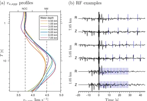
Figure 6.(a) Estimatedvs,appprofiles with corner periodTfor synthetic tests for two layers (including WC) over oceanic PREM. Each model contains a 7 km thick layer of NOC and an NM up to a depth of 155.05 km. The water depth varies from 0.55 to 7.05 km. (b) Example RF for water depths 1.05, 5.05 and 7.05 km. The arrival times of the water multiples for each corresponding water depth are indicated by blue lines.

(8)

Figure 7. Synthetic test for three to five layers (including WC) over PREM. Detailed model description can be found in Table3and used parameters in Table1.

Left column shows used velocity models with depth below seafloor (b.s.f.). Right column shows estimatedvs,appprofiles with corner periodTfor models in left panel.S-wave velocity of NOC and NM used for forward calculation are given by dashed lines. The velocity of the LVL introduced in the model is indicated by a dotted line. (a) Models andvs,appprofiles for a 1 km thick LVL at different depths in the crust. (b) Models andvs,appprofiles for a 50 km thick LVL at different depths in the mantle. (c) Models andvs,appprofiles for an LVL with different thickness at a depth of 30 km b.s.f. in the mantle.

Table 5. Events used for theP-wave polarization analysis, origin time, hypocentre location and moment magnitudeM_wfrom the NEIC catalogue (earthquake.usgs.gov),is the epicentral distance andpis the horizontal slowness as calculated from the AK135 traveltime tables (rses.anu.edu.au/seismology/ak135).

# Origin time

Lat. Lon. Depth Mw p

[dd.mm.yyyy hh:mm:ss] [^◦] [^◦] [km] [s^◦⁻¹] [^◦]

1 24.08.2011 17:46:11 −7.64 −74.53 147.0 7.0 6.14 59.0

2 02.09.2011 10:55:53 52.17 −171.71 32.0 6.9 4.85 86.9

3 02.09.2011 13:47:09 −28.40 −63.03 578.9 6.7 5.32 78.5

4 23.10.2011 10:41:23 38.72 43.51 18.0 7.1 7.78 47.6

5 22.11.2011 18:48:16 −15.36 −65.09 549.9 6.6 6.00 69.1

6 27.12.2011 15:21:56 51.84 95.91 15.0 6.6 5.90 73.5

7 26.02.2012 06:17:19 51.71 95.99 12.0 6.7 5.88 73.6

8 20.03.2012 18:02:47 16.49 −98.23 20.0 7.4 5.98 72.1

9 11.04.2012 08:38:36 2.33 93.06 20.0 8.6 4.44 105.2

10 11.04.2012 22:55:10 18.23 −102.69 20.0 6.5 5.81 74.6

11 17.04.2012 07:13:49 −5.46 147.12 198.0 6.8 1.77 144.7

(9)

for the comparison of the estimatedvs,app profiles of the models with varied water depth and those including an LVL in either crust or mantle. The reference model is depicted with a solid blue line in Figs6(a) and7.

Fig.6shows the influence of the water depth on the appearance of theS-wave velocity profiles. For this test, we create receiver site models including a WC with a thickness from 0.55 to 7.05 km. The models consist of a 7 km thick NOC and a NM (Table1) which extends to a total depth of 155.05 km where PREM takes over. It is visible that the overall appearance of the profiles is similar (Fig.6a).

All profiles have velocities similar to the NOC for periods shorter than 2 s. For longer periods, all profiles show a bump in velocity.

The maximum in velocity is similar or larger than the velocity of the NM and increases for larger water depth. The decrease ofvs,app

below NM velocities at longer periods is probably related to the additional (long period) phases present in the global case (e.g. W phase, Kanamori1993) and/or the possible incomplete deconvolution of the P wave signal at these periods which depends on the Wiener filter parameters (Supporting Information Fig. S3).

The behaviour of the profiles can be explained by the influence of the water multiples which is directly related to their traveltimes.

The thinner the water layer the more water multiples arrive in a shorter time window, for example, for 0.55 km the traveltime of a water multiple is∼0.73 s and for 7.05 km∼9.4 s (vp, WC = 1.5 km s⁻¹ andp=7.78 s/^◦, Fig.6b). The more water multiples arrive in a shorter time window the more the signal of the direct P-wave gets distorted and this has a direct influence on the Wiener filter estimation for the deconvolution. This is visible in Fig.6(b) in which the RF for water depths of 5.05 km and 7.05 km show a series of regular spaced positive and negative spikes onZRFwhich are expected if the directP-wave is properly deconvolved. For a water depth of 1.05 km, no such spike series is observed.

Nevertheless, the water depth has only a minor influence on the appearance of thevs,appprofiles at least for the deep ocean, but a removal of the water multiples (Osenet al.1999; Thorwart & Dahm 2005) before deconvolution might be useful for shallow water depths to prevent influences by wave form distortions.

4.4 Influence of LVL

We test the ability of our method to detect a LVL in different depths in either crust or mantle (Fig.7). All models have again a 5.05 km thick WC as is given by CRUST 1.0 for the area of the deployment (Supporting Information Fig. S1; Laskeet al.2013).

The first three models in Fig.7(a) (CI, CII, CIII, Table 3) consist of a normal oceanic crust (NOC) with a 1 km thick layer of 10 per cent reduced crustal velocities and density (ROC) in three different depths below seafloor (0, 3 and 6 km), and a normal mantle (NM) above PREM. In Fig.7(a), the estimatedvs,app profiles of the three models are quite similar in appearance. For model CI (orange profile in Fig.7a), we find lower velocities for the shorter periods (<0.8 s) compared to the reference model CM-REF (blue profile in Fig.7a). Model CII (yellow profile in Fig.7a) has lower velocities from∼0.7 to∼2 s compared to the reference model. This appearance might also be explained with a model consisting of two solid layers over PREM b.s.f. with a lower crustal velocity than the reference model CM-REF. The last model CIII (purple profile in Fig.7a) shows nearly the same appearance as the reference model CM-REF.

The next six receiver site models (MI-50, MII-50, MIII-50, MIV- 50, MV-50, MVI-50, Table3and Fig.7b) consist of an NOC and

an NM with a 50 km thick layer of 10 per cent reduced mantle velocities and density (RM) in six different depths below seafloor (7, 10, 20, 30, 50 and 100 km). In Fig. 7(b), all profiles show a velocity of∼3.75 km s⁻¹for periods shorter than∼2 s which corresponds very well to theS-wave velocity of the NOC. Thevs,app

profiles for model MI-50 and MII-50 (orange and yellow profile) significantly differ from the reference model (blue profile) for longer periods (>2 s). Both profiles show a bump in velocity, which has a maximum velocity similar to theS-wave velocity of the RM. Nei- ther the profile of MI-50 nor MII-50 show velocities comparable to the NMS-wave velocity. The profile of model MII-50 behaves in a similar way like the profile of the model MI-50. This indicates that the 3 km thick layer of NM in model MII-50 has only small influence on the appearance of the estimatedvs,appprofile. The maximum velocity of the model MII-50 is slightly increased compared to the MI-50 profile. This effect might also be explained with a model similar to MI-50 but with a faster or thicker layer than the 50 km RM.

The other models in Fig.7(b) (MIII-50, MIV-50, MV-50 and MVI-50) show a clear bump in theirvs,appprofiles. Furthermore, their profiles are nearly identical to the CM-REF profile for periods shorter than∼5.6 s. The bump in velocity increases from 4.535 km s⁻¹ to 4.8 km s⁻¹ with the thickness of the upper NM layer (13 km to 93 km). Furthermore, its maximum lies at longer periods the deeper the location of the LVL. The velocities at periods longer than 16 s increase with the depth of the LVL. Despite a larger maximum velocity, the MVI-50 profile has a similar appearance as the CM-REF profile. This indicates a possible trade-off between the depth of the LVL and the uppermost mantle velocity. It might therefore be explained by a model with a higher mantle velocity and no LVL if this would be observed for real (noisy) data (Supporting Information Fig. S2).

At last, we tested the influence of a LVL in the mantle at a depth of 30 km b.s.f. for different layer thickness (1, 5, 10, 20, 50 and 100 km; models MIV-1, MIV-5, MIV-10, MIV-20, MIV-50, MIV- 100, Table3and Fig.7c). The appearance of all tested models in Fig. 7(c) is similar to the models MIII-50, MIV-50, MV-50 and MVI-50 discussed before. All profiles show a similar behaviour to the reference model CM-REF for periods shorter than∼5.6 s. The appearance of the bump in velocity differs. For the models MIV-1 and MIV-5, the profiles are nearly identical to the reference model CM-REF. The profiles of the other four models (MIV-10, MIV-20, MIV-50 and MIV-100) mainly differ in the decrease in velocity with increasing thickness of the LVL for periods longer than∼12 s (Fig.7c).

In conclusion, a thin crustal LVL can be detected in the upper and middle crust, but not in the lower crust (Fig.7a). A thin fast velocity layer or LVL in the uppermost mantle has only minor influence on thevs,appprofile. A clear influence on thevs,appprofile is visible for thicker (>10 km) fast and LVL above∼50 km b.s.f.

4.5 Summary of synthetic tests

We conclude that the overall appearance of thevs,appprofile gives an indication of the number of layers which should be used to model the profile. The method is able to resolve either an increase or a decrease in theS-wave velocity (e.g. Figs4and7) and it is sensitive to the thickness of the layers (e.g. Figs5and7). Furthermore, we find that the water depth has only a minor influence on the appearance of the vs,appprofile (Fig.6). A 1 km thick LVL with 10 per cent reduced crustal velocities and densities is detectable in the upper and middle

(10)

Figure 8. Layout and location of the OBS array. The bathymetry (EMEPC, Task Group for the Extension of the Continental Shelf) is indicated by the colour. The OBS positions are marked with triangles. Station D05 had two clamped components and is not used in the analysis. The distance to the Gloria fault along an N-S profile is given by the white line. The location of the OBS array and the Eurasian–African plate boundary (Gloria Fault, Bird 2003) is shown on the inset map.

crust (0–3 km b.s.f., model CI and CII), but it has only a minor influence on the appearance of thevs,appprofile if it is located in the lower crust (7 km b.s.f., model CIII). A small influence on thevs,app

profiles is also observable for thin (<10 km) fast velocity layers (e.g. MII-50) or LVL (e.g. MIV-1 and MIV-5) in the uppermost mantle but likely remains undetected if the data are not compared to those of undisturbed regions. The appearance of thevs,appprofile is clearly influenced by LVL or fast velocity layers which are at least a few tens of kilometres thick (e.g. MIV-20, MIV-50). We also find that a 50 km thick LVL with 10 per cent reduced mantle velocities and densities has an influence on the appearance of the vs,appprofile if its interface to an upper layer (either NM or NOC) is located at depths above∼50 km b.s.f. (e.g. MI-50, MV-50). On the other hand, it should be noted that the search for a velocity model which explains a givenvs,appprofile is non-unique (e.g. similarity of CIII and CM-REF) due to the trade-off betweenS-wave velocity and layer thickness. In the following section, we present thevs,app

profiles for real OBS data in the Eastern Mid Atlantic and describe a quantitative modelling approach to determine S-wave velocity- depth models which is designed based on the conclusion drawn in this section and the obtainedvs,appprofiles of the real data.

5 A P P L I C AT I O N T O R E A L D AT A 5.1 Data

Within the DOCTAR project (Deep OCean Test ARray), twelve broad-band OBSs were deployed in the Eastern Mid Atlantic (Fig.8) approximately 60 km to 135 km North of the Gloria Fault which is part of the Eurasian–African plate boundary (Bird2003).

The stations recorded seismometer and hydrophone data from July 2011 until April 2012. The array had an aperture of∼75 km

and was located in 4.5 km to 5.5 km water depth. One of the twelve stations had two clamped components (filled red triangle in Fig.8, Hannemannet al.2014), therefore we do not use the data from this station for our analysis. The data are time corrected (Hannemann et al.2014) and the horizontal components are oriented by using Pphases and Rayleigh phases (Stachniket al.2012; Sumyet al.

2015) of know teleseismic events.

For the analysis, we exclude all events for which a strong resonance with periods between 0.5 to 4 s (depending on the station, Figs9a–c for station D03) is observed and for which this resonance has a clear influence on the estimated polarization angle (e.g.

Fig.9d). The observed resonance has a specific period range for each station which can also be identified in the probabilistic power spectral density (PPSD) of all three components by elevated amplitudes (Figs 9a–c at∼3 s for station D03). We think that this resonance is related to the sedimentary cover in which wave energy is trapped. The resonance is triggered by ambient noise as well as body waves (compare Figs9d and e before and after theP-wave arrival). Furthermore, an incomingP-wave at station D03 initially results in a resonance signal on the Z and the R component. Ap- proximately 9 s later, an increasing resonance is observed on the T component (Fig.9e). It is beyond the scope of this study to further describe or analyse this phenomenon. We only analyse events and period ranges for which the earthquake signal is visible in the recordings and stronger than the resonance signal. We also exclude all periods shorter than the corner period of the event recording from the analysis.

We use one to five events at the different stations and analyse in total 33 events at all stations (Tables5and6and Fig.10). We choose the window length for the deconvolution for the (Z, R) RFs for each event based on the quality of the recorded signal. For the damping parameter of the Wiener filter, we use 0.01. Furthermore, we include all apparentP-wave incidence angle measurements in the analysis, for which the SNR on ZRF and RRFis larger than 4 (signal time window [−10 s, 10 s] and noise time window [−55 s,

−25 s] relative to the directPspike). We select the weightwnin eq.

(11) to be the SNR on RRF.

It is likely that serpentinite is present in either the oceanic crust or mantle close to a major transform fault like the Gloria fault (White et al.1992). Therefore, we do not put any constrains onvp/vsratios by using the grid search presented in Section 4 rather than the root search to estimate the medianvs,appprofiles shown in Fig.10. We use the period range between 0.5 and 16.0 s for the analysis, because of the band limited nature of the earthquake signals and a known high self-noise level of the used instruments for periods longer than 10 s (St¨ahleret al.2016, and Figs9a–c). In order to show the variability of the results, we obtain thevs,appprofiles for each event (Tables5and6) and each tested densityρ1(1.0–6.0 g cm⁻³ in 0.1 g cm⁻³ steps). We define a grid with cells centred at all used corner periodsTl and all possible apparentS-wave velocities vs,app and count the crossings (hits) of allvs,app profiles for each grid cell (grey-scale plots in Fig.10). This visualization gives the opportunity to get an idea about the uncertainties of the obtained result. We observe that the real data estimates forvs,appoften show a multimodal distribution for each periodTlwhich represents the individual events. Therefore, the median profile of the total misfit and the weighted hit-count of the individual event’s estimates are, in our opinion, a better representation of the result and its uncertainties than the mean and its standard deviation.

TheS-wave velocities of NOC and NM are given by the dashed grey lines in Fig. 10. This shows that for the majority of the OBS (except D07 and D10, Figs10f and i) the shorter periods