Structure of the oceanic lithosphere and upper mantle north of the Gloria fault in the eastern mid-Atlantic by receiver function analysis
Katrin Hannemann1, Frank Kr¨uger2, Torsten Dahm2,3, Dietrich Lange1
Katrin Hannemann, khannemann@geomar.de
1GEOMAR Helmholtz Centre for Ocean Research Kiel, Wischhofstr. 1-3, 24148 Kiel, Germany
2Institute of Earth and Environmental Science, University of Potsdam,
Karl-Liebknecht-Str.24-25, 14476 Potsdam, Germany
3Section 2.1, Physics of Earthquakes and Volcanoes, GFZ Potsdam, Helmholtzstr.
6/7, 14467 Potsdam, Germany
This article has been accepted for publication and undergone full peer review but has not been through the copyediting, typesetting, pagination and proofreading process, which may lead to differences between this version and the Version of Record. Please cite this article as doi: 10.1002/2016JB013582
Abstract. Receiver functions (RF) have been used for several decades to study structures beneath seismic stations. Although most available sta- tions are deployed on-shore, the number of ocean bottom station (OBS) ex- periments has increased in recent years. Almost all OBSs have to deal with higher noise levels and a limited deployment time (∼1 year), resulting in a small number of usable records of teleseismic earthquakes. Here, we use OBSs deployed as mid-aperture array in the deep ocean (4.5-5.5 km water depth) of the eastern mid-Atlantic. We use evaluation criteria for OBS data and beam forming to enhance the quality of the RFs. Although some stations show re- verberations caused by sedimentary cover, we are able to identify the Moho signal, indicating a normal thickness (5-8 km) of oceanic crust. Observations at single stations with thin sediments (300-400 m) indicate that a probable sharp lithosphere-asthenosphere boundary (LAB) might exist at a depth of
∼70-80 km which is in line with LAB depth estimates for similar lithospheric
ages in the Pacific. The mantle discontinuities at ∼410 km and ∼660 km are clearly identifiable. Their delay times are in agreement with PREM. Over- all the usage of beam formed earthquake recordings for OBS RF analysis is an excellent way to increase the signal quality and the number of usable events.
Keypoints:
• First evidence of a normal mantle transition zone in the mid-Atlantic from RFs in the deep ocean
• Improve signal quality of OBS receiver functions (RFs) by quantitative evaluation and beam forming
• Body wave imaging of discontinuities in mid oceanic lithosphere and up- per mantle using OBS data
1. Introduction
More than 70% of the Earth is covered by oceans, and the majority of the oceanic crust is not affected by recent volcanic or tectonic activities like mid-ocean ridges, sub- duction zones or hot spots. The P wave velocity-depth structure of the oceanic crust and uppermost mantle has been characterized by active geophysical experiments [e.g. White et al., 1992]. Deeper structures in the oceanic lithosphere and upper mantle are studied using broadband ocean bottom stations [OBSs, e.g. Suetsugu and Shiobara, 2014]. In recent years, several passive large-scale experiments with OBSs have been conducted [e.g Friederich and Meier, 2008; Barruol and Sigloch, 2013; Gao and Schwartz, 2015; Lin et al., 2016; Ryberg et al., 2017]. Nevertheless, most of the OBS studies are located at mid-ocean ridges [e.g Shen et al., 1998a; Tilmann and Dahm, 2008; Jokat et al., 2012;
Grevemeyer et al., 2013; Hermann and Jokat, 2013; Schlindwein et al., 2013, 2015], hot spots [e.g. Suetsugu et al., 2007; Barruol and Sigloch, 2013; Davy et al., 2014; Geissler et al., 2016;Ryberg et al., 2017], subduction zones [e.g Suetsugu et al., 2010; Kopp et al., 2011;Laigle et al., 2013;Ruiz et al., 2013;Grevemeyer et al., 2015;Janiszewski and Abers, 2015] or the transition from continental crust to oceanic crust [e.g.Czuba et al., 2011;Grad et al., 2012; Libak et al., 2012; Suckro et al., 2012; Monna et al., 2013; Altenbernd et al., 2014; Kalberg and Gohl, 2014], and are thus not representative of undisturbed oceanic crust and mantle.
Most of our knowledge of the oceanic mantle is based on global surface wave tomography [e.g.Romanowicz, 2009], with rather good path coverage in the oceans but low resolution for sharp discontinuities. Furthermore, studies using land based stations at teleseismic
distances have been conducted to analyze underside reflections to resolve oceanic mantle structures [PP and SS precursors, Gossler and Kind, 1996; Gu et al., 1998; Flanagan and Shearer, 1998;Gu and Dziewonski, 2002; Deuss et al., 2013;Saki et al., 2015]. Both methods lack spatial resolution. On the other hand, receiver function (RF) analysis provides a strong tool to image discontinuities in the lithosphere and the upper mantle down to the transition zone with high lateral resolution [e.g Vinnik, 1977; Langston, 1979]. So far only a limited number of receiver function (RF) studies of undisturbed oceanic lithosphere have been conducted using 500 m deep borehole stations and OBSs [Suetsugu et al., 2005; Kawakatsu et al., 2009;Olugboji et al., 2016].
This study focuses on OBS RFs in the eastern mid-Atlantic in the vicinity of the Eurasian-African plate boundary, in which – to our knowledge – no OBS RF study has previously been done. We target major discontinuities within the oceanic lithosphere and mantle. The Mohoroviˇci´c discontinuity (Moho) marks the boundary between oceanic crust and mantle and is expected in depths between 5-8 km [e.g. White et al., 1992].
Thickened or thinned oceanic crust may be related to over-thrusting, under-plating, or basin formation. The RF phase of the Moho arrives only one or two seconds after the dominant P phase [e.gKawakatsu et al., 2009], and therefore requires high-frequency data [Audet, 2016], and a good signal-to-noise ratio (SNR). Furthermore, it is often masked by sediment reverberations which hamper a direct interpretation of the Moho signal [Audet, 2016; Kawakatsu and Abe, 2016].
The lithosphere-asthenosphere boundary (LAB) beneath the oceans is often imaged using surface waves [e.g Romanowicz, 2009; Takeo et al., 2013, 2016; Lin et al., 2016], SS waveforms [e.g. Rychert et al., 2012], RFs employing land stations [e.g. Li et al., 2000;
Kumar and Kawakatsu, 2011], or OBSs [e.g.Kawakatsu et al., 2009;Olugboji et al., 2016].
Most of the discussed models of the LAB [Kawakatsu et al., 2009; Fischer et al., 2010;
Olugboji et al., 2013] include thermal control, changes in rheology, dehydration, anisotropy or partial melt. Experiments with polycrystalline materials [Takei et al., 2014; Yamauchi and Takei, 2016] at subsolidus temperatures indicate that solid state mechanism such as diffusionally accommodated grain boundary sliding play an important role for S wave velocity decrease with rising temperature in the oceanic lithosphere [figure 20 inYamauchi and Takei, 2016]. Besides the depth of the LAB, the sharpness of the discontinuity is of interest. A relatively smooth transition would be expected if the position of the LAB is purely thermally controlled [Olugboji et al., 2013], and a sharp boundary if it is controlled by composition [e.g. abrupt change in water content, Karato and Jung, 1998]. Both of these cases mark end-member models, and a variety of intermediate models may be possible (e.g. a gradual change in the water content leading to a smooth transition). For example, a land based S wave RF study of oceanic lithosphere in subduction zones [Kumar and Kawakatsu, 2011] supports the model of thermal control, but the observed scatter in the observations indicates additional controlling factors. Observations of the oceanic LAB indicate a diffuse age-dependent boundary in young oceans and a sharp age-independent LAB at ∼70 km in old oceans [e.g. Fischer et al., 2010; Karato, 2012; Olugboji et al., 2013]. A sub-solidus model which assumes grain boundary sliding [Karato, 2012;Olugboji et al., 2013] predicts a transition from an age-dependent diffuse LAB roughly following the 1300 K isotherm in young oceans, to a sharp discontinuity at constant depth in old oceans. The age at which this transition happens, depends on the thermal model used
for the modeling, and lies between 40-80 Ma [Karato, 2012] or 55-75 Ma [Olugboji et al., 2013].
The Lehmann discontinuity is assumed to mark the lower boundary of the asthenosphere [e.g.Lehmann, 1961;Dziewonski and Anderson, 1981;Deuss et al., 2013]. It is located at around 220 km depth, and its cause is still debated [Karato, 1992;Deuss and Woodhouse, 2004]. Only a few RF [Shen et al., 1998a] and SS precursor observations [Deuss and Woodhouse, 2002] exist of the oceanic Lehmann discontinuity.
The three global mantle discontinuities at approximately 410 km, 520 km and 660 km depth (referred to as ’410’, ’520’ and ’660’, respectively) are associated with phase tran- sitions in olivine or the aluminum phases (e.g. garnet) of the mantle [e.g Agee, 1998;
Helffrich, 2000; Deuss et al., 2013]. In the ocean, the mantle transition zone (MTZ), de- fined by the ’410’ and the ’660’, has mostly been studied by using PP and SS precursors [Gossler and Kind, 1996;Gu et al., 1998; Flanagan and Shearer, 1998;Gu and Dziewon- ski, 2002; Deuss et al., 2013; Saki et al., 2015]. There are also some global RF studies of the MTZ [Chevrot et al., 1999; Lawrence and Shearer, 2006; Tauzin et al., 2008] and local studies focusing on the MTZ using OBS data [Shen et al., 1998a;Gilbert et al., 2001;
Suetsugu et al., 2005, 2007, 2010]. Some global studies of SS precursors suggest a thinner MTZ beneath the oceans than below the continents [Gossler and Kind, 1996; Gu et al., 1998; Gu and Dziewonski, 2002], however Flanagan and Shearer [1998] (SS precursors) andChevrot et al.[1999] (RF) could not observe such a correlation. The lack of correlation is also confirmed by local studies [Shen et al., 1998a, b; Silveira et al., 2010].
Here, we use data from eleven OBSs located in the eastern mid-Atlantic approximately 100 km North of the Gloria Fault (Figure 1b) to investigate the structure of the oceanic
crust and upper mantle using array techniques [e.g. “delay and sum“ beam forming, Rost and Thomas, 2002] and receiver functions. OBS data is usually characterized by a small amount of good quality events within a short recording period of the deployed instruments [∼1 year, Webb, 1998]. One of the main reasons is the often low signal-to- noise ratio (SNR) at ocean bottom stations [Webb, 1998;Dahm et al., 2006], especially in the horizontal components. There have been different strategies to increase the number of usable events: either by reinstalling the OBS at the same site [e.g. Cascadia Initiative, Janiszewski and Abers, 2015], or recently by using array techniques [Thomas and Laske, 2015]. The latter is known to increase the SNR of an event by coherent stacking of the observed signals [Rost and Thomas, 2002]. It uses the event’s azimuth and the slowness of the considered phase for the estimation of time delays between the stations which are then removed before stacking the single station recordings [beam forming, for further details Rost and Thomas, 2002]. The experiment presented here is designed in such way that the stations form a mid-aperture array with inter-station distances of 10-20 km and a maximum aperture of 75 km (Figure 1b). This design allows us to stack all stations to enhance phases originating from the deeper parts of the upper mantle. Additionally, we employ a quality control by using evaluation criteria such as relative spike position within the deconvolution time window and search for an optimal deconvolution length to improve the SNR of each RF. Furthermore, we analyze the RFs from single OBSs, stacks of all stations and beams in different frequency bands, and compare amplitudes and delay times of the RFs with synthetic data.
2. Data
We use recordings of eleven OBSs that were installed in the deep sea (4.5-5.5 km water depth) of the eastern mid-Atlantic in 2011 (Figure 1b). These stations are equipped with three component broad-band seismometers (Guralp CMG-40T, 60 s - 50 Hz) and hydrophones (HighTechInc HTI-04-PCA/ULF, 100 s - 8 kHz, flat instrument response down to 5 s, at D08 down to 2 s) and recorded 100 Hz data. To obtain an accurate clock drift, we use ambient noise cross-correlation and compare it to the drift calculated from the synchronization with GPS to reveal static time offsets [Hannemann et al., 2014].
Subsequently, we use the pyrocko toolbox (emolch.github.io/pyrocko) to apply a time correction by inserting and deleting samples. A twelfth station (D05) has not been used for the analysis because of two clamped seismometer components.
For the free fall OBSs used in this study, the orientation of the vertical component is aligned by a gimbaling system [St¨ahler et al., 2016]. Since for the OBS data the orientation of the horizontal components is unknown, we test P phase polarization and Rayleigh and Love waves [Thorwart, 2006;Stachnik et al., 2012;Sumy et al., 2015] to align the horizontal components to the north and east (see appendix A for details).
We use in the following the results of the P phase for the rotation of the horizontal traces, because we find from a frequency-wavenumber analysis with a moving time window using the vertical traces [Rost and Thomas, 2002] that the estimated back-azimuths of the P phases are more precise than those of the Rayleigh phases. They show on average a smaller deviation from the expected back-azimuths [see also Thorwart, 2006].
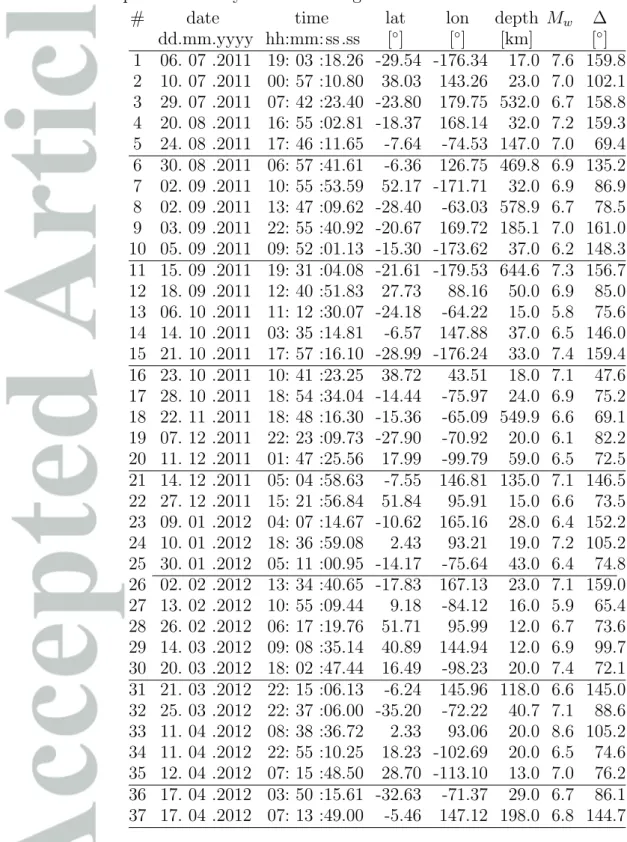
For the RF calculation, we examine all events that have a body wave detection in our frequency-wavenumber detector with values of P between ∼30◦-90◦ epicentral distance, Pdiff between ∼90◦-110◦ epicentral distance and PKPdf between ∼140◦-160◦ epicentral
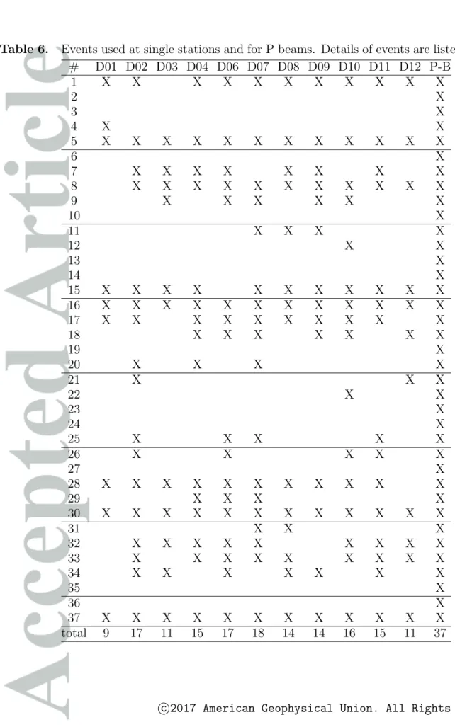
distance. The events finally used (single: 25, beams: 37, see Tabs 5 and 6 in the appendix) are chosen based on the evaluation criteria described below.
3. Methods
When the up-going compressional wave (P wave) is incident on an interface within the Earth, its upward propagating energy is partitioned into a P wave and a vertical polarized shear wave (SV wave). The latter is also referred to as P-to-S (Ps) wave conversion and is a secondary phase which arrives later than the direct P phase (i.e. the refracted P waves).
The amplitudes of the Ps conversions are typically several tens of times smaller than those of the direct P phase, depending on the S wave velocity change at the discontinuity and the incidence angle [e.g. Chevrot et al., 1999; Juli`a, 2007]. The relative Ps amplitudes can be calculated from the ratio of the refraction coefficient ´PP´x and ´PS´x for which x indicates the depth of the discontinuity [seeAki and Richards, 2002, for definition of acute accents]. In addition to the problem of small relative amplitudes, the identification of Ps phases is often obscured by ambient noise and multiple reflections beneath the receiver.
Therefore, specific deconvolution and stacking methods were developed to enhance the signal-to noise ratio (SNR) of the weak Ps phase [Vinnik, 1977; Langston, 1979].
We calculate RFs in the vertical-radial coordinate system, ZRT [Z = vertical, R = horizontal radial, T = horizontal transversal, e.g. Hannemann et al., 2016]. For the rotation into ZRT, we use the theoretical azimuth obtained using the station position and the hypo-center of the corresponding earthquake (see Tab. 5 in the appendix). The P wave signal on the Z component is used to determine a time domain Wiener filter [e.g.
Kind et al., 1995] which transforms the rather complex P wave signal into a band limited spike signal. The filter is then applied to the R component to obtain the ZR RF.
For the estimation of the Wiener filter, we use the built-in function “spiking” of Seismic Handler [Berkhout, 1977;Stammler, 1993] which is able to calculate an optimum lag spik- ing filter [Robinson and Treitel, 1980; Yilmaz, 2008]. This function offers the possibility to use either the centroid of the signal, tc (center of mass, eq. 1), as the spike position or a user-specified spike position. In this study, we use the centroid of the signal,tc, as spike position, which is similar to the effective wavelet length as proposed byBerkhout [1977]:
tc= PN
i=1i· |ai| PN
i=1|ai| . (1)
The centroid of the signal,tc, is calculated for a deconvolution time window containing N amplitude samples using the sample number, i, and the amplitude, ai, of the i-th sample.
The inversion to determine the Wiener filter (inverse filter) works best for minimum phase signals [e.g. Scherbaum, 2001]. As P wave signals are usually mixed phase signals, we stabilize the inversion matrix with a damping factor (0.01). The resulting RF shows several spikes representing converted phases and their multiples from different interfaces/
discontinuities. The spikes of the secondary phases should be separated from the spike of the direct phase [Vinnik, 1977; Langston, 1979]. The amplitudes and delay times of the spikes of the secondary phases constrain the S wave velocity changes, their multiples the impedance contrast, and both the depths of the interfaces under investigation [e.g.
Juli`a, 2007]. The deconvolution removes the source time function from the RFs, so that RFs from different events can be stacked after the traces have been stretched to represent time functions on a common ray path. For this distance moveout correction [Yuan et al., 1997], we use a reference distance of 67◦ and a global velocity model [oceanic PREM, Dziewonski and Anderson, 1981].
The determination of RFs at OBSs may be influenced by water multiples [e.g.Thorwart and Dahm, 2005] or noise [tilt or water wave compliance, e.g. Bell et al., 2015] which can be corrected on the vertical component by using hydrophone data [e.g. Thorwart and Dahm, 2005;Bell et al., 2015] or the horizontal components [e.g.Bell et al., 2015]. We do not observe water multiples in our teleseismic recordings and therefore we do not apply any correction for them. Furthermore, the water wave compliance is only present at very low frequencies (∼100 s) in 4.5-5.5 km water depth [e.g. Crawford et al., 1998;Bell et al., 2015]. We avoid this frequency band by high-pass filtering the RFs. The tilt noise cannot be excluded in our case and might influence the RFs at periods longer than∼10 s. Tilting [e.g. movement of the OBS frame by currents, Webb, 1998; Crawford et al., 1998; Bell et al., 2015] has a higher influence on the horizontal components than on the verticals and a correction of the vertical component [e.g.Bell et al., 2015] would probably lead to rather similar results for the estimated RFs [e.g. Janiszewski and Abers, 2015]. We therefore do not remove the tilt noise from the vertical component.
We find that the SNR of a RF is mainly determined by the quality of the earthquake recording and the length of the deconvolution time window used for the determination of the Wiener filter. To obtain RFs with sufficient SNR, we follow two approaches: (1) increase the SNR of earthquake recordings by employing “delay and sum” beam forming [Rost and Thomas, 2002] using either the plain recordings, or normalize the recordings to the root mean square (rms) amplitude of the noise (-200 s to -100 s before P onset) on a single component to optimize destructive interference of noise amplitudes, and (2) introduce a quality control which employs a set of evaluation criteria to select a subset of deconvolution lengths for single station recordings and beams. A beam forming approach
using OBS data is not common and to our knowledge, our study is the first to apply this technique before the calculation of OBS RFs. We employ the normalization of the earthquake recordings to the rms amplitude of the noise on the Z component to improve the signal used for the deconvolution and on the R component to suppress the noise on the horizontal components.
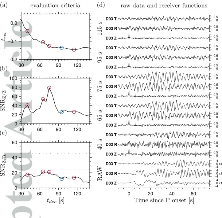
To determine whether the chosen time window contains a mainly minimum phase signal or mainly noise, we choose as first evaluation criterion the spike position, trel, relative to the deconvolution time window,tdec:
trel = tc− tdec2
tdec . (2)
In the case of a mainly minimum phase signal, the spike position is located within the first half of the deconvolution time window (tc < tdec2 ⇒ trel < 0). On the other hand, if the time window contains mainly noise, the spike position is in the middle of the deconvolution time window (tc≈ tdec2 ⇒trel ≈0).
The success of the deconvolution is estimated by the SNR of the Z component of the RF (SNRZ/Z), which is the second evaluation criterion used. It is determined by estimating the ratio of the squared rms amplitudes in the signal time window (-10 s to 10 s relative to P spike) and noise time window (-55 s to -25 s before P spike) on the Z component.
In order to quantify the success of resolving upper mantle discontinuities, the third and last evaluation criterion is the ratio of the squared rms amplitudes of the signal time window on the Z component of the RF and the noise time window on the R component of the RF (SNRZ/R). We compare this to the theoretical ratios of the refraction coefficients
P´P´410
P´S´410 and P´´P´660
PS´660 assuming PREM velocities [Dziewonski and Anderson, 1981]. We test
different deconvolution time window lengths, tdec, starting with 30 s and increasing the length in 5 s steps to a time window length which approximately equals the time difference between the P onset and the PP phase arrival. The deconvolution length for each single event recording and beam is chosen by the following four steps:
1.trel<0 for mainly minimum phase signals (Figs. 2a and 3a) 2. SNRZ/Z &10 for a good deconvolution (Figs. 2b and 3b)
3. SNRZ/R & PP´´PS´´660660 and/ or SNRZ/R & PP´´PS´´410410 for resolving upper mantle discontinuities (Figs. 2c and 3c)
4. manual revision of remaining RFs (Figs. 2d and 3d)
The fourth step (manual revision) is required to exclude RFs which are influenced by high-frequency noise or ringing. These disturbed RFs are often hard to distinguish from undisturbed RFs with the simple evaluation criteria employed here.
We observe a small time shift in the first peak on the R component (Fig. 2d) that can be explained by the influence of a sedimentary cover [Sheehan et al., 1995]. We calculated the mean pre-event noise spectra and P wave spectra of all used events (Tabs 5 and 6) using the ZRT components of the single stations and the beams without normalization (Fig. 11 in the appendix). The spectra show that there is often a change in spectral characteristics between pre-event noise spectra and P wave spectra. Furthermore, there is evidence for sedimentary reverberations at some stations (D01-D06). Moreover, a probabilistic power spectral density analysis [PPSD, McNamara, 2004] reveals a resonance like effect on all three seismometer components of each station [Hannemann et al., 2016]. These effects are also visible in the raw data in Figure 2d and are probably related to signal and ambient noise induced reverberations in the sedimentary cover at each station [Hannemann et al.,
2016]. The interpretation of RFs can be hampered by the presence of such reverberations and must therefore be done carefully [Audet, 2016; Kawakatsu and Abe, 2016]. Further- more, the ZRT coordinates are preferred for the calculation of RFs at OBSs, as the usage of the ray-oriented coordinate system (LQT) may lead to a large amplitude at 0 s on the Q component of the LQ RFs in the presence of sediment reverberations [e.g. Olugboji et al., 2016] which cannot be modeled by using a 1D velocity-depth model.
Using the events from Tabs 5 and 6, we find that beam forming improves – as expected – the SNRZ/Z and the SNRZ/R (Figure 3) and that this effect can be enhanced by a nor- malization of the individual traces before stacking (red and blue lines compared to yellow lines in Figures 3b-c). We get the highest SNRZ/Z values of the tested normalizations for the RFs of the beams with a pre-normalization to the rms amplitude of the noise on the Z component (ZNR). On the other hand, the highest SNRZ/R of the tested normalizations is observed for the RFs of the beams with a pre-normalization to the rms amplitude of the noise on the R component (RNR). We therefore present only the ZR RFs for the beams with pre-normalization to the noise on either the Z or R component (ZNR or RNR) in the following analysis. Furthermore, we find that in our study 2-4 times more events are usable for the RF analysis utilizing beams than in the case of a single OBS (Tab. 6).
For the RF analysis, we perform a bootstrap [Efron and Tibshirani, 1986] to estimate the uncertainties of the picked delay times and the confidence levels of the RF amplitudes. For this purpose, we randomly choose the RFs before stacking the distance moveout corrected traces and repeat this procedure for 300 trials [e.g. Suetsugu et al., 2010]. Furthermore, we use the amplitudesbi(t) at timetof the total number of bootstrapped traces (M=300)
to calculate the standard errorσ(t) [Deuss, 2009] of the amplitude of the stacked RFd(t) at timet:
σ(t) = s
PM
i=1[d(t)−bi(t)]2
M(M −1) . (3)
We indicate the 95% confidence levels of the RFs by plotting twice the standard error σ(t) for the presented RF stacks. For a better visibility, we shade the areas beneath
positive amplitudes in blue for which the lower confidence level is larger than zero and the areas above negative amplitudes in red for which the upper confidence level is smaller than zero (e.g. Fig. 4a). Since the data in our OBS network has a higher noise level compared to most land stations, such a rigorous analysis and visualization of uncertainties is very helpful for the interpretation.
4. Results and discussion
In this study, we determine the time difference between the converted (Ps) and the direct (P) phase (hereafter referred to as the delay time) on move-out corrected, stacked receiver functions (RFs) of several earthquakes. In the following, we discuss the observed Ps phases from different depth levels and discontinuities in the crust and upper mantle.
4.1. Structure of the oceanic crust
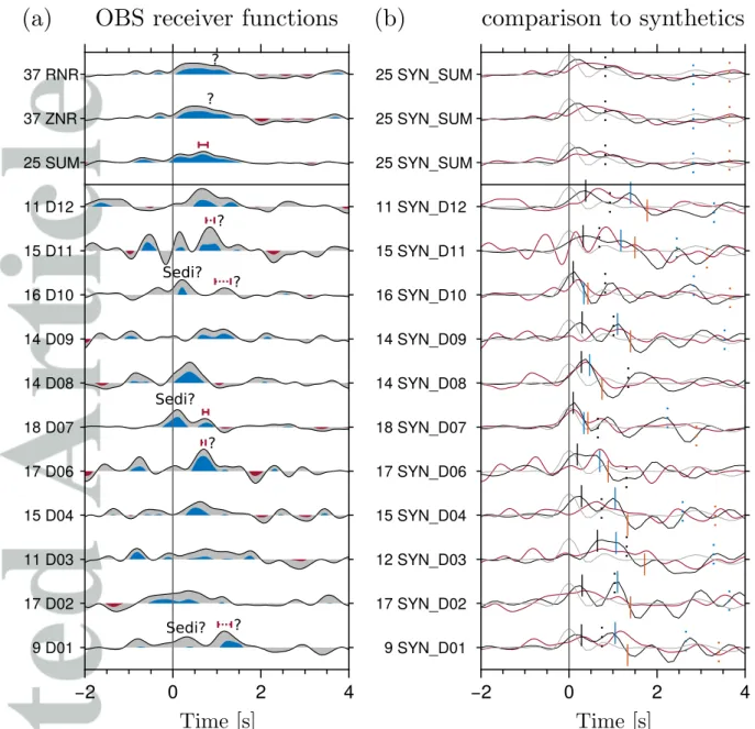
In Figure 4a, we show the bandpass filtered (0.5 s to 60 s) ZR RFs for the single OBSs (D01-D12), the stack of all stations (SUM) and the stack of the beam formed traces (ZNR and RNR). In addition, we present in Figure 4b the comparison with synthetic RFs calculated for velocity-depth models obtained by P wave polarization analysis [black, Hannemann et al., 2016] which consist of a sedimentary, a crustal and an uppermost
mantle layer over PREM, and a simple model without a sediment layer and an oceanic crustal thickness of 7 km (gray). As previously stated, the time shift of the first peak on the RFs indicates the presence of a sedimentary layer and is also visible in the mismatch between the OBS RFs and the synthetics obtained for the 7 km thick oceanic crust.
The presence of a sedimentary cover as estimated by Hannemann et al. [2016] leads to a complex interference pattern of sediment and Moho phases and multiples in the first seconds of the RFs (compare the black curves in Figure 4b). This biasing effect of a sedimentary cover often restricts the direct interpretation of OBS RFs [Audet, 2016], as discussed by Kawakatsu and Abe [2016].
In a comparison with the synthetic data (Figure 4b), we identify a positive early arrival on the ZR RFs of the stations D01, D07 and D10, and probably D08 which may be related to the sediment layer. The delay times at D01 (∼0.3 s) and D07 (∼0.1 s) match well with the theoretical delay times of the models obtained by Hannemann et al. [2016]
(D01: 0.28 s, D07: 0.09 s). At station D10, the first positive amplitude arrives slightly later (∼0.2 s) than predicted by the synthetic model [0.09 s, Hannemann et al., 2016].
This may be caused by the poorly resolved sediment layer in the model for station D10 [Hannemann et al., 2016]. At station D08, the synthetic RF suggests that the first peak is likely a mixture of several phases. In general, mismatches between the synthetics calculated with the sediment models obtained by Hannemann et al.[2016], and the OBS data are found particularly for those stations at which the sediment model is based on only few P wave recordings, i.e. in case of the stations D09 and D12.
For the identification of the Moho and the determination of its robustness, we use the information provided by the comparison of the ZR RFs with the synthetic data (Fig-
ure 4b), and the 95% confidence level. In conclusion, we find one single station within the array (D07) at which we are confident about the identified Moho (Figure 4). First of all, the lower confidence level identifies this peak as being robust for all bootstrapped traces. Secondly, the OBS RFs and the synthetic RFs have a similar appearance which indicates low influence of noise on the RFs. There is some evidence for the presence of a Moho-related signal at other single stations (D01, D06, D10 and D11), but the comparison with the synthetic data and the estimated confidence levels indicate that these are biased by the interference with sediment related signals.
Furthermore, the ZR RF stacks of all stations provides an estimate for an average Moho delay time (0.68 s, Figure 4a). Although the beam formed traces ZNR and RNR show comparable amplitudes to the stack of all stations (SUM), we cannot clearly identify the Moho signal on these beam traces. This is probably related to the effect of the interference of the reverberations originating from the different sedimentary models at the individual stations in the beam formed traces which leads to the observed broad peak in the RF beams.
We estimate theoretical Ps delay times for depth intervals of 2 km using the PREM velocity model [Dziewonski and Anderson, 1981] and a slowness of 6.4 s/◦, which cor- responds to a distance of 67◦, which was also used for the moveout correction. Based on these values, we estimate pseudo-depths using the obtained Moho delay times. This results in depths of 4.8-5.1 km for station D07 and the stack of all stations (SUM). This crustal thickness is less than the expected values for oceanic crust [e.gWhite et al., 1992;
Laske et al., 2013] and slightly less than the values obtained byHannemann et al.[2016].
In addition, we marked a possible PpPs Moho multiple at ∼3.4 s and a possible PpSs
Moho multiple at∼4.8 s on the stacks of properly time shifted ZNR RF stacks which have been binned in the slowness domain (bins of 0.5 s/◦ every 0.25 s/◦) before the moveout correction (Figure 5). The delay times of these multiples correspond well to an interface at∼7-8 km depth which agrees with the expected thicknesses for oceanic crust [e.gWhite et al., 1992; Laske et al., 2013]. This indicates that the later arriving crustal multiples may be less disturbed by sediment reverberations than the direct Moho phase.
4.2. Lithosphere-asthenosphere boundary (LAB)
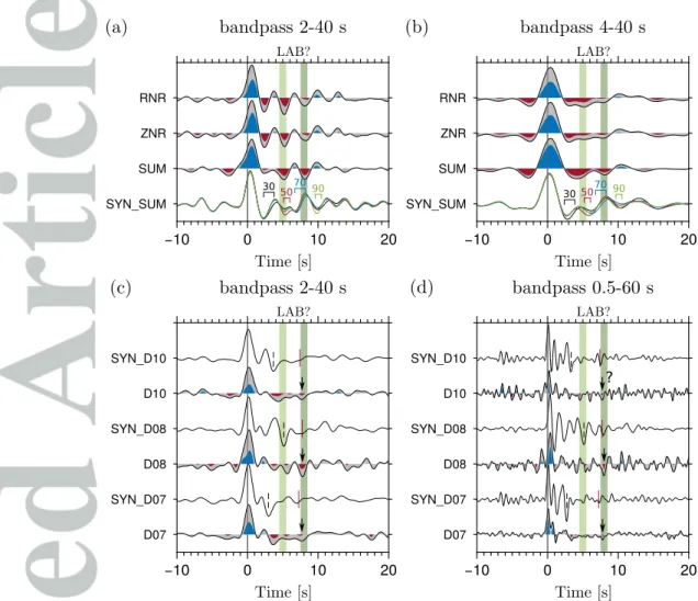
In Figure 6, we present the ZR RFs filtered in two different period bands (2-40 s in Figure 6a and 4-40 s in Figure 6b) to discuss negative phases which might be associated with the lithosphere-asthenosphere boundary (LAB). First of all, we observe an oscillation with a dominant period of ∼3 s at most single stations (e.g. D01-D06, D11 and D12 in Figure 6a). This is likely related to sediment and crustal reverberations and has a large influence on the overall appearance of the RFs. The RFs at the stations D07-D10 show fewer indications for the presence of strong sedimentary and crustal reverberations after
∼4 s. On the other hand, at station D09 we observe strong acausal amplitudes similar to
stations D06 and D11. Station D09 might therefore also be problematic for the further analysis of possible LAB phases. At stations D07, D08 and D10, we observe small negative phases at ∼8 s for the filter band between 2 s and 40 s which tend to merge with the neighboring phases for the filter band between 4 s and 40 s. A negative phase at ∼8 s is also visible at stations D02, D03, D04 and D06, but at these stations it is likely related to the strong sediment and crustal reverberations. In the stack of all stations (SUM) and the normalized beam traces (ZNR and RNR), we observe negative phases at ∼5 s and
∼8 s indicated by faint green areas in Figure 6. The phase at ∼5 s is likely related to the
PpPs multiple of the Moho (Figure 5) and the phase at ∼8 s is probably a combination of the already discussed reverberations at most of the stations, and the negative phase at similar times observed at stations D07, D08 and D10. If these phases were related to discontinuities in the subsurface, the delay times would correspond to interfaces at depths of 40-50 km (∼5 s) and 65-75 km (∼8 s).
Figure 12 (in the appendix) shows stacks of all single station RFs, which have been stacked in 0.5 s/◦ slowness bins, depending on their slowness. Furthermore, we indicate the delay times of an interface at 40-50 km depth (light green area in Figure 12 in the appendix) and at 65-75 km depth (dark green area in Figure 12 in the appendix) assuming PREM [Dziewonski and Anderson, 1981]. A clear move-out is not observable for the negative phase at∼5 s, but might be possible for the phase at ∼8 s, although we observe several multiples arriving at similar times (e.g. for slowness 4-5 s/◦ at ∼8-9 s). These multiples are probably related to sedimentary and crustal structures. Just based on this slowness bin stack, we cannot determine whether one of the negative phases at∼5 s and
∼8 s is related to the LAB.
We model synthetic ZR RFs for different LAB depths (Figure 7) to further investigate the interference of the sedimentary and crustal multiples and a sharp LAB (velocity drop of ∼11.3% from vs=4.51 km/s to vs=4 km/s). The models obtained by P wave polarization [Hannemann et al., 2016] have been used for the upper 10.5 km. From depths of 10.5 km to 20.5 km, we use a gradient from the uppermost mantle velocities in the corresponding model, to “normal” mantle velocities (vp=8.12 km/s,vs=4.51 km).
We use the same station and event distribution as for the OBS data. In Figures 7a and b, we compare the stack of all stations (SUM) and the normalized beams (ZNR and RNR)
with a stack of all synthetic RFs (SYN SUM) for different LAB depths (black: 30 km, red: 50 km, blue: 70 km and green: 90 km). The synthetics show a similar influence of the sediment and crustal reverberations on the overall appearance of the RFs as the OBS data. Furthermore, the effect of the LAB at different depths on the RFs is often only identifiable by the direct comparison with the other models (e.g. LAB at 30 km depth for bandpass 2-40 s, Figure 7a) due to the interference with the sediment and crustal reverberations. The LAB signal in the stack of all stations is therefore masked by the influence of the different sedimentary and crustal structures at the single stations.
A quantitative modeling of LAB depth and velocity reduction at the LAB would first of all require an in-depth analysis of the sedimentary and crustal structure at the single stations, in order to properly model the sediment and crustal reverberations. The stack of the current synthetics shows a time shift in the first peak compared to the real data, which indicates that the models probably underestimate the sediment effect. Furthermore, we notice that during the modeling done so far, not all effects of the sedimentary and crustal structure which are observed at the OBSs can be modeled with 1D velocity-depth models (e.g. the aforementioned resonance). Based on our experiences with data quality and modeling effort, the ability of detailed quantitative modeling to capture the sediment and crustal reverberations remains unclear and such modeling is therefore beyond the scope of this study. We have to conclude from Figures 7a and b that we are not able to give a depth estimate for the LAB for the whole working area by using the stacks of all stations and the normalized beams.
Nevertheless, the single stations D07, D08 and D10 – as was already pointed out – are less influenced by strong sedimentary and crustal reverberations, which is also visible
in the P wave spectra (Figures 11f, g and i). From the P wave polarization analysis [Hannemann et al., 2016], we know that the sediments are rather thin (300-400 m) at these stations. Most of the sediment and crustal multiples therefore arrive before ∼4 s and do not interfere with the later arriving negative phase at ∼8 s. Furthermore, the comparison between the synthetics and the OBS RFs in Figure 4 (bandpass 0.5-60 s) showed that they agree quite well in the first seconds at stations D07, D08 and D10. In Figure 7c, we observe that the shape of synthetics for an LAB at 70 km and the real data is comparable in the first seconds for the filter band between 2 s and 40 s. The synthetics also show that the PpSs multiple of the Moho is a much stronger negative phase at ∼3- 5 s, in comparison to the later arriving LAB phase (∼7-7.5 s). Furthermore, the LAB phase is hard to identify in this filter band due to the interference with other multiples.
For shorter periods (bandpass 0.5-60 s, Figure 7d), we can identify small negative phases at ∼8 s at D07, D08 and D10, although the phase at D10 remains questionable due to similar earlier negative phases. Nevertheless, we have to be aware that at these short periods we are approaching the limits of resolution of our data, therefore we have to be careful with interpreting the observations. The observed phases at∼8 s (marked by black arrows in Figures 7c and d) arrive a bit later than the LAB phases in the corresponding synthetic RFs and indicate a probable sharp LAB. Their delay times correspond to LAB depths between 70 km and 80 km if the sediment and crustal structure obtained by P wave polarization is assumed at the single stations. For a lithospheric age between 75 Ma and 85 Ma as in this study [Figure 9, afterM¨uller et al., 2008], the observation of an LAB in 70-80 km depth would be in line with depth observations made for similar ages in the Pacific [figure 6 in Rychert et al., 2012].
In summary, we conclude that there might be a probable sharp LAB at ∼70-80 km, for which we find weak evidence at single stations with rather thin sediments (300-400 m).
Furthermore, we notice that strong sedimentary and crustal reverberations mask the ar- rival of the LAB phase and need to be considered in the discussion or modeling of potential LAB phases.
4.3. Upper mantle discontinuities
The Ps converted phases caused by the ’410’ and ’660’ should arrive ∼44 s and ∼68 s after the direct P phase and have positive amplitudes. These amplitudes are several tens of times smaller than the direct P phase (compare P´´P´410
PS´410 and P´´P´660
PS´660 in Figure 2c).
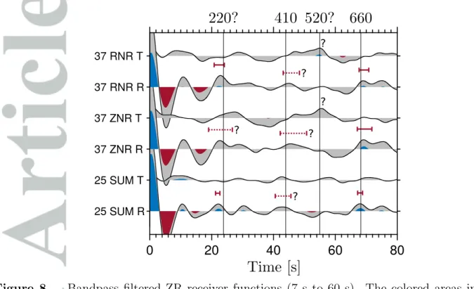
The usual approach to enhance them is stacking. In Figure 8, we present the bandpass filtered (7-60 s) stacked ZR RFs of the single stations (SUM) and beam formed traces with different pre-normalizations (ZNR and RNR). The delay times shown as guidance correspond to depths of 220 km, 410 km, 520 km and 660 km assuming PREM [Dziewonski and Anderson, 1981]. For the upper mantle, we can clearly identify one positive phase at ∼68-69 s and a second low confidence phase at ∼43-46 s. We associate the phase at
∼43-46 s with the ’410’ and the phase at∼68-69 s with the ’660’.
The expected delay time for the ’410’ assuming PREM velocities is 43.97 s, which agrees quite well with the measured delay times of the stacks of the single stations (43.11±1.26) and is similar to the measured delay times of the beam formed traces (ZNR: 46.46±2.13, RNR: 45.76±1.31). This indicates a normal depth of the ’410’, which is in good agreement with observations made bySaki et al.[2015] in their precursor study. The expected delay time for the ’660’ assuming PREM is 68.26 s. The measured delay times are similar (SUM: 68.01±0.41, ZNR: 69.46±1.18 and RNR: 69.26±0.78). Although Saki et al.[2015]
provide only a few depth estimates for the ’660’, our observations match their PP precursor estimates North and South of our OBS array. Transforming delay times of the mantle discontinuities to pseudo-depths is usually strongly influenced by the velocity model of the uppermost mantle and crust. It is therefore common practice to employ more robust estimates like the delay time difference between the ’660’ and the ’410’ [e.g. Gu and Dziewonski, 2002]. This difference is 24.9±1.33 s for the single station stack (SUM), 23.00±2.44 s for the stack of the beam formed traces normalized to the noise on the Z component (ZNR) and 23.50±1.52 s for the stack of the beam formed traces normalized to the noise on the R component (RNR). This difference between the ’410’ and the ’660’
is similar to the theoretical estimate using PREM (24.29 s) within the error bounds.
A small time shift of the MTZ Ps phases can be observed (∼1.5 s) between the single stations’ stack and the stack of the beam formed traces. We investigate whether this observed time shift of the ’410’ and ’660’ is related to the different processing of the single stations and the beam formed traces by calculating synthetic RFs using a full wave field reflectivity method [QSEIS, Wang, 1999] with our station distribution, a global velocity model [PREM Dziewonski and Anderson, 1981] and a local crustal model [CRUST1.0 Laske et al., 2013]. We find no difference in the estimated delay times of the mantle discontinuities for the beam formed traces stack and the stack of the single stations. The small time shift in the delay times between the single stations stack and the beam formed traces stack (Fig. 8) may therefore indicate a difference in the velocities or the thicknesses of the lithosphere and mantle above the ’410’ sampled by the according rays.
Examining the map showing the piercing points (Figure 9), we find that the RFs mostly sample structures within the Eurasian plate (north of the Gloria fault) for back-azimuths
between ∼200◦ to 80◦. The azimuthal coverage is similar for the single stations and the beam formed traces. It is therefore likely that the small time shift between the different stacks is caused by the method specific differences in the weighting according to the noise (i.e. the pre-normalization to the rms amplitude of the noise).
There is another low confidence signal at a delay time of ∼22-23 s. This signal arrives slightly earlier than would be expected for a depth of 220 km in PREM (23.81 s, Figure 8).
The association of this phase with the Lehmann discontinuity is difficult, as it has a low confidence level and likely interferes with crustal and lithospheric multiples (see first 20 s in Figures 6a and b and Figure 8).
In addition, a low confidence, weak signal is visible at ∼56 s on the T components of the beam formed traces, the arrival of which is delayed compared to the expected arrival of the ’520’ from PREM (54.92 s, see Figure 8). Onsets on the T component of RFs can be caused by dipping layers or shear wave splitting in anisotropic layers [e.g. Cassidy, 1992;Savage, 1998;Farra and Vinnik, 2000]. The oceanic upper mantle is anisotropic in global models like PREM and shows lateral and depth dependent variations of anisotropy in surface wave based tomography models [Pilidou et al., 2005]. However, it is hard to identify signals on the R component (Figure 8) which might represent a split shear wave component near the T component signal at ∼56 s. If this signal originates due to anisotropy in a layer above 520 km depth, shear waves converted at 660 km depth should be split as well. This is not observable in Figure 8. The limited number of available RFs, as well as their often low signal quality hinder the formation of back-azimuth dependent stacks with a sufficient confidence level. The latter would be required to constrain a
possible anisotropy component in the data. The cause of this signal therefore remains enigmatic.
In summary, the usage of beamforming techniques increases the number of events avail- able for the RF analysis and therefore also the SNR of the RF. In combination with bootstrapping and uncertainty estimations, they help to estimate the confidence of sig- nals originating from deeper mantle structures as the MTZ.
5. Conclusion
This study shows that it is possible to identify discontinuities in the oceanic crust and upper mantle down to the MTZ using OBS data. Furthermore, it explores the advantages of using beam forming to improve the signal quality of RFs and a quality control employing evaluation criteria such as relative spike position and SNR to search for the optimal deconvolution length. In this study, we demonstrate that these techniques work well.
The first analyzed discontinuity is the Moho, for which the average pseudo-depth is
∼5 km estimated using PREM velocities. This is slightly less than would be expected
for oceanic crust in general [e.g White et al., 1992; Laske et al., 2013]. The RFs show evidence for the presence of a sediment layer at the single stations which likely influences the estimated delay times and therefore the pseudo-depths. Furthermore, possible crustal multiples indicate a Moho depth of ∼7-8 km which is more in line with the expected values [e.gWhite et al., 1992; Laske et al., 2013].
Secondly, we focus on the asthenosphere. The interpretation of the LAB and the Lehmann discontinuity is difficult because of simultaneously arriving reverberations of sediment, crustal and lithospheric structures, and requires synthetic modeling to under-
stand the observed effects. The synthetic modeling indicates that the influence of sedi- mentary and crustal reverberations masks the arrival of the LAB phase for the stack of all stations and the normalized beams. Nevertheless, at single stations with thin (300-400 m) sediments a weak negative phase indicates a probable sharp LAB at ∼70-80 km depth.
These estimates are in line with depth estimates for similar ages in the Pacific [Rychert et al., 2012]. A positive phase arrival at ∼22-23 s on the RF stacks may correspond to the Lehmann discontinuity [e.g. Deuss et al., 2013], but likely interferes with crustal and lithospheric multiples.
We find that the ’410’ and the ’660’ are located at depths expected from PREM and are in line with a recent precursor study in this area [Saki et al., 2015]. A delay between the ’410’ and the ’660’ signal observed at the single stations stack and the beam formed traces stack is likely caused by the different pre-normalization of the data before the RF calculation.
In conclusion, this study shows that the number of usable events for RF studies at the ocean bottom can be more than doubled in comparison to single station approaches using beam forming techniques at a mid-aperture array. This approach is especially promising if deeper mantle features with small amplitudes are to be investigated as it increases the SNR of the event recordings and the number of usable events for the analysis of OBS RFs.
The application of evaluation criteria supports the selection of optimal deconvolution time window lengths. Nevertheless, a manual revision of the RFs resulting from the pre-selected deconvolution lengths is still necessary to exclude RFs from the analysis that are influenced by high-frequency noise. Furthermore, this study proves that the combination of single OBSs and beam forming techniques gives the opportunity to investigate structures from
the sea floor down to the MTZ. The analysis of the local S wave velocity structure via P wave polarization [Hannemann et al., 2016] proves to be useful in understanding the effects encountered by sedimentary and crustal reverberations at single OBSs using synthetic modeling.
Appendix A: Orientation
We test two different approaches to estimate the orientation of the OBSs (i.e. angle between geographic North and the North component of the seismometer): (1) using the P wave polarization on the horizontal components, and (2) using the phase shift of the Rayleigh wave between the vertical and radial components. For the analysis of the P wave polarization, we measure the amplitudes of several teleseismic P phases on all three components for each station. We estimate the theoretical amplitude distribution of the P phase on the horizontal components by using the vertical P wave polarization and the known back-azimuth of the earthquake. After a stepwise rotation of the theoretical amplitude distribution, we calculate the difference (misfit) between the theoretical and the measured horizontal amplitudes.
We estimate this misfit for several events and calculate the mean and standard deviation.
We use the definitions of mean, µ, and standard deviation, σ, from directional statistics analogous to Grigoli et al. [2012] for N measurements of the orientation angle, ϕi, with weightwi, which is chosen based on event quality.
µ= arctan Q
P
∧ σ=p
2·(1−R) (A1)
with P =
N
X
i=1
wicosϕi ∧ Q=
N
X
i=1
wisinϕi
and R= 1
PN i=1wi
pP2+Q2
Furthermore, we combine the misfit functions of all events by calculating the mean of the different misfit functions for each tested angle.
We also use surface waves to estimate the orientation of the stations [Stachnik et al., 2012]. The data are filtered with a bandpass between 20 and 60 s and the horizontal com- ponents are rotated using the back-azimuth of the events. If the horizontal components are properly oriented, the vertical trace will be identical to the Hilbert transform of the radial trace within the time window of the Rayleigh phase [Stachnik et al., 2012]. We decide to include the Love phase in our analysis, because its energy should completely vanish from the radial component if the components have the correct orientation. We use a normalized zero-lag cross correlation, Srz, between the Hilbert transform of the radial trace ( ˜R) and the vertical trace (Z) [equation (A2),Stachnik et al., 2012;Zha et al., 2013].
Srz = ρ(R,Z˜ )
ρ(Z,Z) (A2)
with ρ(X, Y) =Rt2
t1 X(t)Y(t)dt Herein, ρ
R, Z˜
is the zero-lag cross-correlation between the Hilbert transform of the radial trace and the vertical trace and ρ(Z, Z) is the zero-lag auto-correlation of the vertical trace. Before calculating Srz, we normalize the traces. The horizontal traces are
traces in one degree steps and calculate Srz. As for the P phase, we estimate Srz for several events and calculate the mean and standard deviation according to equation (A1).
Furthermore, we append all event data and process them together.
Moreover, we use the bootstrap method and equation (A1) to estimate mean and stan- dard deviation for the combined misfit function for the P phase and the correlation coeffi- cient for the Rayleigh phase. The resulting angles are presented in Tab. 3 for the P phase and in Tab. 4 for the Rayleigh phase and in Figure 10.
Appendix B: Additional Figures
Appendix C: Event tables
Acknowledgments. The authors thank the DEPAS pool for providing the instruments for the DOCTAR project which was funded by the DFG (KR1935/13, DA 478/21-1) and by the Leitstelle f¨ur Mittelgroße Forschungsschiffe (Poseidon cruises 416 and 431).
The authors thank EMEPC (Task Group for the Extension of the Continental Shelf) for providing the bathymetric data and Luis Batista for sharing them. The data processing was partly done using Seismic Handler [Stammler, 1993]. Some figures were created using GMT [Wessel et al., 2013]. The authors thank two anonymous reviewers for their constructive comments on the manuscript. We thank Jess Hillman who helped to improve the language of the paper. The sea floor seismological data were archived by Alfred Wegener Institute (AWI), Helmholtz Centre for Polar Research, Bremerhaven, Germany and are available upon request. The clock drifts of the OBSs are published inHannemann et al. [2014] and the orientations in appendix A of this study (Tab. 3).
References
Agee, C. B. (1998), Phase transformations and seismic structure in the upper mantle and transition zone, inUltrahigh-Pressure Mineralogy. Physics and Chemistry of the Earth’s Deep Interior, vol. 37, edited by R. J. Hemley and P. H. Ribbe, chap. 5, pp. 165–203, Mineralogical Society of America, Washington, D.C.
Aki, K., and P. G. Richards (2002),Quantitative Seismology, 2nd ed., 700 pp., University Science Books, doi:10.1016/S0065-230X(09)04001-9.
Altenbernd, T., W. Jokat, I. Heyde, and V. Damm (2014), A crustal model for northern Melville Bay, Baffin Bay, Journal of Geophysical Research B: Solid Earth, 119(12), 8610–8632, doi:10.1002/2014JB011559.
Audet, P. (2016), Receiver functions using OBS data: promises and limitations from numerical modelling and examples from the Cascadia Initiative, Geophysical Journal International, 205(3), 1740–1755, doi:10.1093/gji/ggw111.
Barruol, G., and K. Sigloch (2013), Investigating La R´eunion Hot Spot From Crust to Core, Eos, Transactions American Geophysical Union, 94(23), 205–207, doi:
10.1002/2013EO230002.
Bell, S. W., Y. Ruan, and D. W. Forsyth (2015), Shear Velocity Structure of Abyssal Plain Sediments in Cascadia, Seismological Research Letters, 86(5), 1247–1252, doi:
10.1785/0220150101.
Berkhout, A. J. (1977), Least-squares inverse filtering and wavelet deconvolution, Geo- physics, 42(7), 1369–1383, doi:10.1190/1.1440798.
Bird, P. (2003), An updated digital model of plate boundaries,Geochemistry, Geophysics, Geosystems, 4(3), 1027, doi:10.1029/2001GC000252.
Cassidy, J. J. F. (1992), Numerical experiments in broadband receiver function analysis, Bulletin of the Seismological Society of America, 82(3), 1453–1474.
Chevrot, S., L. Vinnik, and J. P. Montagner (1999), Global-scale analysis of the mantle Pds phases, Journal of Geophysical Research, 104(B9), 20,203–20,219, doi:
10.1029/1999JB900087.
Crawford, W. C., S. C. Webb, and J. A. Hildebrand (1998), Estimating shear velocities in the oceanic crust from compliance measurements by two-dimensional finite differ-
ence modeling, Journal of Geophysical Research: Solid Earth, 103(B5), 9895–9916, doi:10.1029/97JB03532.
Czuba, W., M. Grad, R. Mjelde, A. Guterch, A. Libak, F. Kr¨uger, Y. Murai, and J. Schweitzer (2011), Continent-ocean-transition across a trans-tensional margin seg- ment: Off Bear Island, Barents Sea, Geophysical Journal International, 184(2), 541–
554, doi:10.1111/j.1365-246X.2010.04873.x.
Dahm, T., F. Tilmann, and J. Morgan (2006), Seismic Broadband Ocean-Bottom Data and Noise Observed with Free-Fall Stations: Experiences from Long-Term Deployments in the North Atlantic and the Tyrrhenian Sea, Bulletin of the Seismological Society of America, 96(2), 647–664, doi:10.1785/0120040064.
Davy, C., G. Barruol, F. R. Fontaine, K. Sigloch, and E. Stutzmann (2014), Tracking major storms from microseismic and hydroacoustic observations on the seafloor, Geo- physical Research Letters, 41(24), 8825–8831, doi:10.1002/2014GL062319.
Deuss, A. (2009), Global observations of mantle discontinuities using SS and PP precur- sors, Surveys in Geophysics, 30(4-5), 301–326, doi:10.1007/s10712-009-9078-y.
Deuss, A., and J. H. Woodhouse (2002), A systematic search for mantle dis- continuities using SS-precursors, Geophysical Research Letters, 29(8), 90–94, doi:
10.1029/2002GL014768.
Deuss, A., and J. H. Woodhouse (2004), The nature of the Lehmann discontinuity from its seismological Clapeyron slopes,Earth and Planetary Science Letters,225(3-4), 295–304, doi:10.1016/j.epsl.2004.06.021.
Deuss, A., J. Andrews, and E. Day (2013), Seismic Observations of Mantle Discontinuities and Their Mineralogical and Dynamical Interpretation, inPhysics and Chemistry of the
Deep Earth, edited by S.-i. Karato, pp. 297–323, John Wiley & Sons, Ltd.
Dziewonski, A. M., and D. L. Anderson (1981), Preliminary reference Earth model, Physics of the Earth and Planetary Interiors, 25(4), 297–356, doi:10.1016/0031- 9201(81)90046-7.
Efron, B., and R. Tibshirani (1986), Bootstrap methods for standard error, confidence intervals, and other measures of statistical accuracy, Statistical Science, 1(1), 54–75, doi:10.1214/ss/1177013817.
Farra, V. V., and L. Vinnik (2000), Upper mantle stratification by P and S receiver functions, Geophysical Journal International, 141(3), 699–712, doi:10.1046/j.1365- 246x.2000.00118.x.
Fischer, K. M., H. A. Ford, D. L. Abt, and C. A. Rychert (2010), The Lithosphere- Asthenosphere Boundary,Annual Review of Earth and Planetary Sciences,38(1), 551–
575, doi:10.1146/annurev-earth-040809-152438.
Flanagan, M. P., and P. M. Shearer (1998), Global mapping of topography on transition zone velocity discontinuities by stacking SS precursors,Journal of Geophysical Research, 103(B82), 2673–2692, doi:10.1029/97JB03212.
Friederich, W., and T. Meier (2008), Temporary Seismic Broadband Network Acquired Data on Hellenic Subduction Zone, Eos, Transactions American Geophysical Union, 89(40), 378, doi:10.1029/2008EO400002.
Gao, H., and S. Schwartz (2015), Preface to the Focus Section on Cascadia Ini- tiative Preliminary Results, Seismological Research Letters, 86(5), 1235–1237, doi:
10.1785/0220150160.
Geissler, W. H., W. Jokat, M. Jegen, and K. Baba (2016), Thickness of the oceanic crust, the lithosphere, and the mantle transition zone in the vicinity of the Tristan da Cunha hot spot estimated from ocean-bottom and ocean-island seismometer receiver functions, Tectonophysics, doi:10.1016/j.tecto.2016.12.013.
Gilbert, H. J., A. F. Sheehan, D. A. Wiens, K. G. Dueker, L. M. Dorman, J. Hilde- brand, and S. Webb (2001), Upper mantle discontinuity structure in the region of the Tonga Subduction Zone, Geophysical Research Letters, 28(9), 1855–1858, doi:
10.1029/2000GL012192.
Gossler, J., and R. Kind (1996), Seismic evidence for very deep roots of continents,Earth and Planetary Science Letters,138(1-4), 1–13, doi:10.1016/0012-821X(95)00215-X.
Grad, M., R. Mjelde, W. Czuba, A. Guterch, and the IPY Project Group (2012), Elastic properties of seafloor sediments from the modelling of amplitudes of multiple water waves recorded on the seafloor off Bear Island, North Atlantic,Geophysical Prospecting, 60(5), 855–869, doi:10.1111/j.1365-2478.2011.01022.x.
Grevemeyer, I., T. J. Reston, and S. Moeller (2013), Microseismicity of the Mid- Atlantic Ridge at 7◦S-8◦15’S and at the Logatchev Massif oceanic core complex at 14◦40’N-14◦50’N, Geochemistry, Geophysics, Geosystems, 14(9), 3532–3554, doi:
10.1002/ggge.20197.
Grevemeyer, I., E. Gr`acia, A. Villase˜nor, W. Leuchters, and A. B. Watts (2015), Seis- micity and active tectonics in the Alboran Sea, Western Mediterranean: Constraints from an offshore-onshore seismological network and swath bathymetry data, Journal of Geophysical Research: Solid Earth, 120(12), 8348–8365, doi:10.1002/2015JB012073.
Grigoli, F., S. Cesca, T. Dahm, and L. Krieger (2012), A complex linear least-squares method to derive relative and absolute orientations of seismic sensors,Geophysical Jour- nal International, 188(3), 1243–1254, doi:10.1111/j.1365-246X.2011.05316.x.
Gu, Y. J., and A. M. Dziewonski (2002), Global variability of transition zone thickness, Journal of Geophysical Research,107(B7), 2135, doi:10.1029/2001JB000489.
Gu, Y. J., A. M. Dziewonski, and C. B. Agee (1998), Global de-correlation of transition zone discontinuities, Earth and Planetary Science Letters, 157(1-2), 57–67.
Hannemann, K., F. Kr¨uger, and T. Dahm (2014), Measuring of clock drift rates and static time offsets of ocean bottom stations by means of ambient noise, Geophysical Journal International, 196(2), 1034–1042, doi:10.1093/gji/ggt434.
Hannemann, K., F. Kr¨uger, T. Dahm, and D. Lange (2016), Oceanic lithospheric S- wave velocities from the analysis of P-wave polarization at the ocean floor, Geophysical Journal International, 207(3), 1796–1817, doi:10.1093/gji/ggw342.
Helffrich, G. (2000), Topography of the transition zone seismic discontinuities,Reviews of Geophysics, 38(1), 141–158, doi:10.1029/1999RG000060.
Hermann, T., and W. Jokat (2013), Crustal structures of the boreas basin and the knipovich ridge,north atlantic, Geophysical Journal International, 193(3), 1399–1414, doi:10.1093/gji/ggt048.
Janiszewski, H. A., and G. A. Abers (2015), Imaging the Plate Interface in the Cascadia Seismogenic Zone: New Constraints from Offshore Receiver Functions, Seismological Research Letters,86(5), 1261–1269, doi:10.1785/0220150104.
Jokat, W., J. Kollofrath, W. H. Geissler, and L. Jensen (2012), Crustal thickness and earthquake distribution south of the Logachev Seamount, Knipovich Ridge,Geophysical
Research Letters,39(8), 2–7, doi:10.1029/2012GL051199.
Juli`a, J. (2007), Constraining velocity and density contrasts across the crust-mantle boundary with receiver function amplitudes,Geophysical Journal International,171(1), 286–301, doi:10.1111/j.1365-2966.2007.3502.x.
Kalberg, T., and K. Gohl (2014), The crustal structure and tectonic development of the continental margin of the Amundsen sea embayment, West Antarctica: Implica- tions from geophysical data, Geophysical Journal International, 198(1), 327–341, doi:
10.1093/gji/ggu118.
Karato, S.-i. (1992), On The Lehmann Discontinuity, Geophysical Research Letters, 19(22), 2255–2258, doi:10.1029/92GL02603.
Karato, S.-i. (2012), On the origin of the asthenosphere, Earth and Planetary Science Letters, 321-322, 95–103, doi:10.1016/j.epsl.2012.01.001.
Karato, S.-i., and H. Jung (1998), Water, partial melting and the origin of the seismic low velocity and high attenuation zone in the upper mantle, Earth and Planetary Science Letters, 157(3-4), 193–207, doi:10.1016/S0012-821X(98)00034-X.
Kawakatsu, H., and Y. Abe (2016), Comment on ”Nature of the Seismic Lithosphere- Asthenosphere Boundary within Normal Oceanic Mantle from High-Resolution Receiver Functions” by Olugboji et al., Geochemistry, Geophysics, Geosystems, 17(8), 3488–
3492, doi:10.1002/2016GC006418.
Kawakatsu, H., P. Kumar, Y. Takei, M. Shinohara, T. Kanazawa, E. Araki, and K. Suye- hiro (2009), Seismic Evidence for Sharp Lithosphere-Asthenosphere Boundaries of Oceanic Plates, Science,324(5926), 499–502, doi:10.1126/science.1169499.
Kind, R., G. L. Kosarev, and N. V. Petersen (1995), Receiver functions at the stations of the German Regional Seismic Network (GRSN), Geophysical Journal International, 121(1), 191–202, doi:10.1111/j.1365-246X.1995.tb03520.x.
Kopp, H., W. Weinzierl, A. Becel, P. Charvis, M. Evain, E. R. Flueh, A. Gailler, A. Galve, A. Hirn, A. Kandilarov, D. Klaeschen, M. Laigle, C. Papenberg, L. Planert, and E. Roux (2011), Deep structure of the central Lesser Antilles Island Arc: Relevance for the formation of continental crust,Earth and Planetary Science Letters,304(1-2), 121–134, doi:10.1016/j.epsl.2011.01.024.
Kumar, P., and H. Kawakatsu (2011), Imaging the seismic lithosphere-asthenosphere boundary of the oceanic plate,Geochemistry, Geophysics, Geosystems, 12(1), Q01,006, doi:10.1029/2010GC003358.
Laigle, M., A. Hirn, M. Sapin, A. B´ecel, P. Charvis, E. Flueh, J. Diaz, J. F. Lebrun, A. Ges- ret, R. Raffaele, A. Galv´e, M. Evain, M. Ruiz, H. Kopp, G. Bayrakci, W. Weinzierl, Y. Hello, J. C. L´epine, J. P. Viod´e, M. Sachpazi, J. Gallart, E. Kissling, and R. Nicolich (2013), Seismic structure and activity of the north-central Lesser Antilles subduction zone from an integrated approach: Similarities with the Tohoku forearc,Tectonophysics, 603, 1–20, doi:10.1016/j.tecto.2013.05.043.
Langston, C. A. C. A. (1979), Structure under Mount Rainier, Washington, inferred from teleseismic body waves,Journal of Geophysical Research,84(B9), 4749–4762, doi:
10.1029/JB084iB09p04749.
Laske, G., G. Masters, Z. Ma, and M. E. Pasyanos (2013), CRUST1.0 : An Updated Global Model of Earth’s Crust, in Geophys. Res. Abstracts, vol. 15, pp. Abstract EGU2013–2658.
Lawrence, J. F., and P. M. Shearer (2006), A global study of transition zone thick- ness using receiver functions, Journal of Geophysical Research, 111(6), B06,307, doi:
10.1029/2005JB003973.
Lehmann, I. (1961), S and the Structure of the Upper Mantle, Geophysical Journal In- ternational,4(Supplement 1), 124–138, doi:10.1111/j.1365-246X.1937.tb07108.x.
Li, X., S. V. Sobolev, R. Kind, X. Yuan, and C. Estabrook (2000), A detailed receiver function image of the upper mantle discontinuities in the Japan subduction zone,Earth and Planetary Science Letters,183(3-4), 527–541, doi:10.1016/S0012-821X(00)00294-6.
Libak, A., R. Mjelde, H. Keers, J. I. Faleide, and Y. Murai (2012), An integrated geo- physical study of Vestbakken Volcanic Province, western Barents Sea continental mar- gin, and adjacent oceanic crust, Marine Geophysical Research, 33(2), 185–207, doi:
10.1007/s11001-012-9155-3.
Lin, P.-y. P., J. B. Gaherty, G. Jin, J. A. Collins, D. Lizarralde, R. L. Evans, and G. Hirth (2016), High-resolution seismic constraints on flow dynamics in the oceanic astheno- sphere, Nature, 535(7613), 538–541, doi:10.1038/nature18012.
McNamara, D. E. (2004), Ambient Noise Levels in the Continental United States,Bulletin of the Seismological Society of America, 94(4), 1517–1527, doi:10.1785/012003001.
Monna, S., G. B. Cimini, C. Montuori, L. Matias, W. H. Geissler, and P. Favali (2013), New insights from seismic tomography on the complex geodynamic evolution of two adjacent domains: Gulf of Cadiz and Alboran Sea, Journal of Geophysical Research:
Solid Earth, 118(4), 1587–1601, doi:10.1029/2012JB009607.
M¨uller, R. D., M. Sdrolias, C. Gaina, and W. R. Roest (2008), Age, spreading rates, and spreading asymmetry of the world’s ocean crust,Geochemistry, Geophysics, Geosystems,
9(4), Q04,006, doi:10.1029/2007GC001743.
Olugboji, T. M., S. Karato, and J. Park (2013), Structures of the oceanic lithosphere- asthenosphere boundary: Mineral-physics modeling and seismological signatures, Geo- chemistry, Geophysics, Geosystems, 14(4), 880–901, doi:10.1002/ggge.20086.
Olugboji, T. M., J. Park, S.-i. Karato, and M. Shinohara (2016), Nature of the seis- mic lithosphere-asthenosphere boundary within normal oceanic mantle from high- resolution receiver functions,Geochemistry, Geophysics, Geosystems,17(4), 1265–1282, doi:10.1002/2015GC006214.
Pilidou, S., K. Priestley, E. Debayle, and ´O. Gudmundsson (2005), Rayleigh wave tomog- raphy in the North Atlantic: High resolution images of the Iceland, Azores and Eifel mantle plumes,Lithos, 79(3-4 SPEC. ISS.), 453–474, doi:10.1016/j.lithos.2004.09.012.
Robinson, E., and S. Treitel (1980), Geophysical signal analysis, Prentice Hall Inc., En- glewood Cliffs, N.J.
Romanowicz, B. (2009), The thickness of tectonic plates., Science (New York, N.Y.), 324(5926), 474–476, doi:10.1126/science.1172879.
Rost, S., and C. Thomas (2002), Array seismology: Methods and applications, Reviews of Geophysics,40(3), 1008, doi:10.1029/2000RG000100.
Ruiz, M., A. Galve, T. Monfret, M. Sapin, P. Charvis, M. Laigle, M. Evain, A. Hirn, E. Flueh, J. Gallart, J. Diaz, and J. F. Lebrun (2013), Seismic activity offshore Mar- tinique and Dominica islands (Central Lesser Antilles subduction zone) from tempo- rary onshore and offshore seismic networks, Tectonophysics, 603(April 2007), 68–78, doi:10.1016/j.tecto.2011.08.006.
Ryberg, T., W. Geissler, W. Jokat, and S. Pandey (2017), Uppermost mantle and crustal structure at Tristan da Cunha derived from ambient seismic noise,Earth and Planetary Science Letters, 471, 117–124, doi:10.1016/j.epsl.2017.04.049.
Rychert, C. A., N. Schmerr, and N. Harmon (2012), The Pacific lithosphere-asthenosphere boundary: Seismic imaging and anisotropic constraints from SS waveforms, Geochem- istry, Geophysics, Geosystems,13(9), 1–18, doi:10.1029/2012GC004194.
Saki, M., C. Thomas, S. E. J. Nippress, and S. Lessing (2015), Topography of up- per mantle seismic discontinuities beneath the North Atlantic: The Azores, Canary and Cape Verde plumes, Earth and Planetary Science Letters, 409, 193–202, doi:
10.1016/j.epsl.2014.10.052.
Savage, M. K. (1998), Lower crustal anisotropy or dipping boundaries? Effects on receiver functions and a case study in New Zealand, Journal of Geophysical Research: Solid Earth, 103(B7), 15,069–15,087, doi:10.1029/98JB00795.
Scherbaum, F. (2001),Of Poles and Zeros,Modern Approaches in Geophysics, vol. 15, 2nd ed., 335 pages pp., Springer Netherlands, Dordrecht, doi:10.1007/978-1-4020-6861-4.
Schlindwein, V., A. Demuth, W. H. Geissler, and W. Jokat (2013), Seismic gap beneath Logachev Seamount: Indicator for melt focusing at an ultraslow mid-ocean ridge?, Geophysical Research Letters, 40(9), 1703–1707, doi:10.1002/grl.50329.
Schlindwein, V., A. Demuth, E. Korger, C. L¨aderach, and F. Schmid (2015), Seis- micity of the Arctic mid-ocean Ridge system, Polar Science, 9(1), 146–157, doi:
10.1016/j.polar.2014.10.001.
Sheehan, A. F., G. a. Abers, C. H. Jones, and A. L. Lerner-Lam (1995), Crustal thickness variations across the Colorado Rocky Mountains from teleseismic receiver functions,