Seismotectonics of the Horseshoe Abyssal Plain and Gorringe Bank, eastern Atlantic Ocean: Constraints from ocean

Seismotectonics of the Horseshoe Abyssal Plain and Gorringe Bank, eastern Atlantic Ocean: Constraints from ocean

bottom seismometer data

Ingo Grevemeyer¹ , Dietrich Lange¹ , Heinrich Villinger² , Susana Custódio³ , and Luis Matias³

1GEOMAR Helmholtz Zentrum für Ozeanforschung, Kiel, Germany,²Fachbereich Geowissenschaften, Universität Bremen, Bremen, Germany,³Instituto Dom Luiz, Faculdade de Ciências, Universidade de Lisboa, Lisboa, Portugal

Abstract

At the eastern end of the Azores-Gloria transform fault system to the southwest of Portugal, the plate boundary between Africa and Iberia is a region where deformation is accommodated over a wide tectonically active area. The region has unleashed large earthquakes and tsunamis, including theM_w~ 8.5 Great Lisbon earthquake of 1755. Although the source region of the 1755 earthquake is still disputed, most proposals include a source location in the vicinity of the Horseshoe Abyssal Plain (HAP), which is bounded by the 5000 m high Gorringe Bank (GB). In this study we characterize seismic activity in the region using data recorded by two local networks of ocean bottom seismometers. The networks were deployed in the eastern HAP and at the GB. The data set allowed the detection of 160 local earthquakes. These earthquakes cluster around the GB, to the SW of Cabo Sao Vicente, and in the HAP. Focal depths indicate deep-seated earthquakes, with depths increasing from 20–35 km (mean of 26.17.2 km) at the GB to 15–45 km (mean 31.5 km10.5 km) under the HAP. Seismic activity thus extends down to levels that are deeper than those mapped by active seismic profiling, with the majority of events occurring within the mantle. Thermal modeling suggests that temperatures of approximately 600°C characterize the base of the seismogenic brittle lithosphere at ~45 km depth. The large source depth and thermal structure support previous suggestions that catastrophic seismic rupture through the lithospheric mantle may indeed occur in the area.

1. Introduction

Great earthquakes with magnitudes of 8.4 or larger are usually megathrust earthquakes that occur in subduc- tion zones, like the circum-Pacific belt or the Sunda arc [e.g.,Kanamori, 1977; http://earthquake.usgs.gov/

earthquakes/world/10_largest_world.php]. A memorable exception is the 1755 Great Lisbon earthquake, with an estimated magnitude of 8.5–8.7 [Martinez-Solares et al., 1979; Johnston, 1996]. The earthquake, which generated a devastating tsunami, hit Portugal, Spain, and Morocco and was widely felt over western Europe. However, the location of the Great Lisbon earthquake source is still debated. A number of offshore locations have been proposed, including the Gorringe Bank [e.g.,Johnston, 1996;Grandin et al., 2007], the Marques de Pombal fault to the SW of Portugal [e.g.,Zitellini et al., 2001], and a proposed subduction mega- thurst in the Gulf of Cadiz [e.g.,Gutscher et al., 2012]. In addition, the Horseshoe Abyssal Plain and the Horseshoe Fault are considered candidate source regions of the Great Lisbon earthquake [e.g., Barkan et al., 2009; Stich et al., 2007]. However, tsunami arrival times may suggest that the source was located closer to the Cabo Sao Vicente [Baptista et al., 2011], the westernmost point of the Algarve, southern Portugal.

Deformation along the oceanic Eurasian-African plate boundary to the west and southwest of Iberia (Figure 1) is forced by the slow NW-SE plate convergence and causes rather diffuse deformation [e.g., Sartori et al., 1994; Hayward et al., 1999], analogous to intraplate deformation identified in the Indian Ocean [Wiens et al., 1985]. Seismicity located by regional land networks collapsed into clusters and lineations that generally do not coincide with geologically mapped faults [Custódio et al., 2015]. The seismicity pattern derived from land seismometers may indeed present robust features. Yet because seismicity occurs far outside of land networks, the true epicenters of earthquake offshore are not accurate and might be shifted several kilometres or even tens of kilometres away from their true epicentral locations [Geissler et al., 2010;

Grevemeyer et al., 2015; 2016]. Therefore, the deployment of offshore seismometers is critical to improve focal parameters, in particular to increase the accuracy of hypocentral parameters.

Journal of Geophysical Research: Solid Earth

RESEARCH ARTICLE

10.1002/2016JB013586

Special Section:

Stress at Active Plate

Boundaries - Measurement and Analysis, and Implications for Seismic Hazard

Key Points:

•Microearthquakes occur down to 45 km and at temperatures of<600°C and rupture a domain of upper mantle, including unroofed continental mantle

•Seismicity occurs at depth greater than reflection seismically mapped faults, which thus may splay out from deep-seated faults

•The distribution of microearthquakes do not provide any evidence for a developing subduction zone but rather indicates shortening

Supporting Information:

•Supporting Information S1

Correspondence to:

I. Grevemeyer, igrevemeyer@geomar.de

Citation:

Grevemeyer, I., D. Lange, H. Villinger, S. Custódio, and L. Matias (2017), Seismotectonics of the Horseshoe Abyssal Plain and Gorringe Bank, eastern Atlantic Ocean: Constraints from ocean bottom seismometer data, J. Geophys. Res. Solid Earth,122, 63–78, doi:10.1002/2016JB013586.

Received 23 SEP 2016 Accepted 3 JAN 2017

Accepted article online 6 JAN 2017 Published online 21 JAN 2017

©2017. American Geophysical Union.

All Rights Reserved.

Here we report results from two offshore deployments (Figure 2) of ocean bottom seismometer (OBS). The first network was deployed from April to October 2012 in the vicinity of the Horseshoe Fault and in the Horseshoe Abyssal Plain (HAP) to the NW of the Coral Patch Ridge (Figure S1 in the supporting information).

The second network was deployed from October 2013 to March 2014 at the Gorringe Bank (GB) (Figure S2).

Both networks were designed to study the relationship between seismicity and morphological features. To investigate the ability to cause seismic hazards, we were particularly interested in the assessment of the thickness of the seismogenic layer (maximum depth of faulting), controlling the size of future catastrophic earthquakes. In addition, we surveyed the rupture process of theM_w= 6.0 Horseshoe earthquake of 2007 to relate its centroid depth to the occurrence of microseismicity.

2. Tectonic Setting

The boundary between the African and Eurasian plates is tectonically segmented between the Azores and the Gibraltar Arc, displaying different modes of deformation. In the vicinity of the Azores islands both extension and strike-slip deformation occur. Farther east, along the Azores-Gloria transform fault zone (AGFZ;

Figure 1), deformation is rather simple and motion is right-lateral [e.g.,Serpelloni et al., 2007]. Eastward of the Gorringe Bank, deformation is more complex and distributed across an ~200 km wide region [e.g.,Sartori et al., 1994;Hayward et al., 1999]. This region is characterized by moderate seismic activity, with most earthquakes grouping in clusters [e.g.,Zitellini et al., 2001;Custódio et al., 2015]. Here the plate boundary runs from the well-defined oceanic domain into an area where continental lithosphere might be involved in plate boundary deformation [Pinheiro et al., 1992;Rovere et al., 2004]. In addition to the well-recorded moderate seismicity, the area has been hit by large earthquakes, which include the largest earthquake in the European historical record, the 1755 Lisbon earthquake [Martinez-Solares et al., 1979;Johnston, 1996], the 1969M= 7.9 Horseshoe earthquake [Fukao, 1973], and the 2007M= 6.0 Horseshoe Fault earthquake [Stich et al., 2007;Custódio et al., 2012]. Focal mechanisms show predominantly reverse and strike-slip fault- ing [e.g.,Serpelloni et al., 2007;Stich et al., 2005;Geissler et al., 2010], in agreement with the oblique plate convergence [e.g.,DeMets et al., 2010].

Figure 1.Tectonic setting of the study area to the SW of Iberia at the eastern terminus of the Azores-Gloria Fault Zone (AGFZ). The white squares are land stations providing onset times of earthquakes. The red dots are epicenters from the EHB catalogue (1900–2008) [Engdahl et al., 1998;Engdahl and Villaseñor, 2002]. The white dots and focal mechanism are solutions from the Global Moment Tensor Project (http://www.globalcmt.org). Seafloor bathymetry is taken fromSmith and Sandwell[1997], seafloor age in millions of years fromMüller et al.[2008], and plate boundary (thick black line) to the west of 12°W is fromBird[2003]. Inset shows plate boundary configuration and plate motions [DeMets et al., 2010].

Structurally, the area includes a number of deep basins where water depth exceeds ~5000 m. These include the Tagus Abyssal Plain (TAP), the HAP, and the Seine Abyssal Plain. In addition, large ridges, rising up to

~100 m water depth, like the GB and the Coral Patch Seamount, separate the basins. The ~200 km long,

~80 km wide, and 5000 m high Gorringe Bank [Auzende et al., 1984], located between the TAP and HAP, is the most prominent feature of the area. It strikes NE-SW, roughly perpendicular to the direction of plate convergence. Rocks from the GB, obtained during the Deep Sea Drilling Project at Site 120 [Ryan et al., 1973], submersible dives and dredging [Auzende et al., 1984;Girardeau et al., 1998], indicate that the GB is mainly composed of serpentinized peridotites with gabbroic intrusions. Dating of the intrusions yielded Ar³⁹/Ar⁴⁰ ages of 1431 Myr [Féraud et al., 1986]. Yet it is generally believed that the GB was mainly uplifted in a period of 10–15 Ma during the Miocene [e.g.,Tortella et al., 1997]. Earlier models suggested that thrusting was related to subduction of Africa below Eurasia, suggesting that the TAP and GB were overthrusting the HAP [e.g.,Purdy, 1975]. However, today multichannel seismic data [Sartori et al., 1994;Tortella et al., 1997] and submersible dives [Girardeau et al., 1998] suggest that the HAP and GB overthrusted the TAP. The estimated shortening associated with the uplift of the GB is on the order of 20 km [Sartori et al., 1994;Galindo-Zaldívar et al., 2003;Jiménez-Munt et al., 2010] to 50 km [Hayward et al., 1999].

Martinez-Loriente et al.[2014] used seismic refraction and wide-angle data, constrained by gravity model- ing, to define geological domains in the area (Figure S3). Their results suggest that the TAP, the GB, and HAP form a domain of Lower Cretaceous exhumed mantle [e.g.,Pinheiro et al., 1992;Rovere et al., 2004;

Sallarès et al., 2013], whereas the area to the south and to the east of the Horseshoe Fault is of oceanic Figure 2.Earthquake epicenters (circles) from the preferred location procedure using a 3-D velocity model based on seismic refraction profiling [Martinez-Loriente et al., 2014]. The grey circles indicate events far outside the network (GAP>270°).

The colored dots represent hypocentral depth of well-located events. Transect A-A⁰shows the location of the seismic refraction profile fromMartinez-Loriente et al.[2014]. A cross section along the seismic velocity model A-A⁰is shown in Figure 5. Note that the 3-D procedure did not include any arrival times from land stations, while 1-D re-locations consider land stations (Figures S1 and S2). The black lines are fault zones, lineaments, and tectonic features [Zitellini et al., 2009]. CPR Coral Patch Ridge; CPS: Coral Patch Seamount; GB: Gorringe Bank; HAP: Horseshoe Abyssal Plain; HF: Horseshoe Fault;

MPB: Marques de Pombal Fault; SAB Seine Abyssal Plain; SVC: Sao Vicente Canyon;TAP: Tagus Abyssal Plain. Lineaments in the vicinity of the CPR are called SWIM lineaments [Zitellini et al., 2009]. Focal mechanisms are given in Table 1. Yellow star is the epicenter of theM_w= 6.0 2007 Horseshoe Fault earthquake. Numbers indicate OBS. Note that OBS04 and OBS28 occupy the same deployment site.

origin [Sallarés et al., 2011;Martinez-Loriente et al., 2014]. In addition, the seafloor of the abyssal plains is cov- ered by an up to 5 km thick layer of sediments [e.g.,Rovere et al., 2004;Sallarés et al., 2011, 2013;Martínez- Loriente et al., 2013].

3. Earthquake Data

3.1. Local Earthquake Data

Two OBS networks were deployed to the SW of Portugal with the goal of studying the local seismic activity in the Horseshoe Abyssal Plain and Gorringe Bank [Grevemeyer, 2015]. Deployment and recovery operations were conducted by using the German research vesselPoseidon. Thefirst network was deployed on 12 and 13 April 2012 and was recovered between 14 and 16 October 2012. Over 6 months, 14 OBS monitored local earthquakes in the eastern Horseshoe Abyssal Plain and across the Horseshoe Fault. All OBS were successfully recovered, but OBS01 and OBS03 failed to record any data and two others stopped logging data approximately 1 month before recovery.

The second network consisted of 15 OBS and was deployed between 7 and 11 October 2013 at the Gorringe Bank. Instruments were recovered between 23 and 26 March 2014. Unfortunately, OBS29 was lost and OBS19 did not provide any data. All other stations provided 5 months of good-quality data.

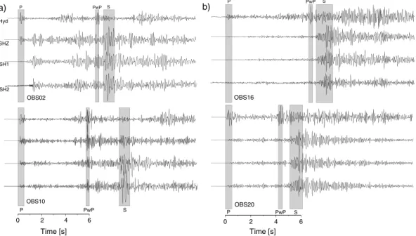
All OBS were equipped with a three-component short-period geophone, with a natural frequency of 4.5 Hz and with a HighTech HTI-04-PCA/ULF hydrophone, recording bothPwave andSwave arrivals (Figures 3 and 4). Continuous waveform data were logged at 50 Hz. The instrument clocks were synchronized to GPS time upon deployment and retrieval; we corrected clock drifts by linear interpolation.

3.2. The 2007 Horseshoe Fault Earthquake

On 12 February 2007 the Horseshoe Abyssal Plain was hit by aM_w5.9 to 6.0 earthquake. The earthquake was previously studied by using regional waveform data [e.g.,Stich et al., 2007;Custódio et al., 2012]. However, it was also recorded at teleseismic distances on stations of world-wide operated seismic networks. We retrieved data from the Incorporated Research Institutions for Seismology (IRIS) data management system for waveform inversion, in order to compute its source properties and centroid depth.

Figure 3.Typical waveform examples from both OBS networks showing typical features for (a) the HAP deployment and (b) the GB deployment. Note that waveforms from the HAP deployment show complex features betweenPandS onsets, likely related to converted energy and multiples caused by reflections within the 4 to 5 km thick sedimentary blanket;P:Pwave onset,PwP: water layer multiple ofPwave;S:Swave onset.

4. Data Processing

4.1. Event Detection, Phase Picking, and Magnitudes

Earthquakes were automatically detected in the continuous time series by using a short-term-average to long-term-average ratio trigger algorithm. An earthquake was detected when six or more stations triggered coincidently. We detected 110 earthquakes by using data from thefirst deployment in the HAP and 54 earthquakes by using data from the second deployment at the GB.

PandSwave arrival onset times were hand-picked. In total, we were able to locate 160 local earthquakes. The averagePwave phase-pick error was estimated at0.12 s;Swave phase-pick errors were much larger, up to 0.50 s. Data from seafloor stations were complemented by phase picks recorded by permanent seismic networks operated in Portugal, Spain, and Morocco, as reported by national catalogues compiled in the International Seismological Centre (ISC) online catalogue.

We computed local magnitudes (Ml) by using the classical approach ofRichter[1935], modified byHutton and Boore[1987]. Accordingly, the magnitude is proportional to the maximum amplitude A of the displacement of a Wood-Anderson seismometer for frequenciesf>1.25 Hz; thus, Ml ~ log₁₀(A). In order to use the Ml scale with instruments other than the Wood-Anderson seismometer, we followed the common practice of measuring the maximum amplitude of the displacement trace in the frequency band 1.25 to 20 Hz.

4.2. Event Location in a 1-D Velocity Model

The nonlinear oct-tree search algorithm NonLinLoc [Lomax et al., 2000] was used to calculate hypocentral parameters. Travel times are computed with thefinite difference solution to the Eikonal equation [Podvin and Lecomte, 1991]. The oct-tree algorithm provides more complete and reliable location uncertainties than linearized inversions, allowing the computation of probability density functions (PDF) for the location of each individual event. The maximum likelihood location is chosen as the preferred location. For each event, NonLinLoc estimates a 3-D error ellipsoid (68% confidence) from the PDF scatter samples. Station correction factors account for localized deviations from the a priori model and are determined from the average residual at each station. For the inversion, the focal depth search was limited to depths below the seafloor, thus avoid- ing“water”quakes for event with poor azimuthal coverage. Most earthquakes occurred at depths>20 km and presented formal epicentral errors of5 km to 18 km and depth errors of6 km to 15 km.

Travel times were initially calculated by using 1-D velocity models. ThePwave velocity structure of both 1-D models was adapted for both networks from the seismic refraction and wide-angle work ofMartinez-Loriente et al.[2014]. In the Horseshoe Abyssal Plain, the velocity structure indicates a 5 km thick sediment layer that overlays unroofed mantle. Velocities in the sediment layer increase from ~1.8 km/s at the seafloor to ~4.5 km/s at the bottom of the sedimentary layer. Basement velocities quickly increase from slightly over 6 km/s to 7 km/s just 2 km below the top of the basement and to>7.5 km/s at a depth of 7 km below the top of the Figure 4.Record section of the hydrophone channel of a Ml = 3.3 earthquake that occurred on 5 July 2012 at 40 km depth below the Horseshoe Abyssal Plain. Time axis was reduced with 8 km/s. Waveforms are plotted as a function of hypocentral distance. Note the fast apparentPvelocity of 8 km/s, indicating that the event occurred within the mantle.

Arrivals at ~7.5 s are multiples of thePonset bouncing in the water column.

basement. At greater depths, velocities are ~8 km/s. Based on these values,Rovere et al.[2004] andMartinez- Loriente et al.[2014] suggest that the basement below the HAP is composed of hydrated mantle.

Samples taken from the Gorringe Bank [Ryan et al., 1973;Auzende et al., 1984;Girardeau et al., 1998] suggest that the GB is mainly composed of serpentinized peridotites with gabbroic intrusions. The seismic velocities inferred for the GB support a thin sedimentary cover overlaying a medium with fast velocities of 4 km/s just 1 km below the seafloor. The core of the bank is characterized by velocities of 5 to 6.5 km/s. At about 10 km depth the medium reaches velocities of 7 km/s, which further increase up to 8 km/s at 18 km depth [Sallarès et al., 2013;Martinez-Loriente et al., 2014]. Overall, the velocity changes under the Gorringe Bank are rather gradual, supporting the presence of unroofed and serpentinized mantle.

In order to reduce the impact of nonmodeled 2-D and 3-D wave-propagation effects, station corrections were calculated and iteratively updated, reducing RMS errors from ~0.4 s in the runs without corrections to<0.15 s for the final re-locations. Station corrections condense local structural variability (site effects) into delay time, removing effects caused by the 3-D structure of the HAP and GB, and hence facilitate clustering of seismicity.

TheSwave velocity structure of the area is poorly known. We therefore used Wadati diagrams (S-Ptime ver- susPtime) in order to infer the local averageV_p/V_sratio [Havskov and Ottemöller, 2000]. To constrain theV_p/V_s ratio, we used all earthquakes with at least eightPandSwave readings, a RMS location misfit of 0.2 or less, and a correlation coefficient of thefit ofS-Ptime versusPtime of>0.9. The resultingV_p/V_sratio was 1.72, sup- porting previous estimates [Custódio et al., 2015]. For the HAP, where OBS data present much more complex waveforms and only a small number ofSwave picks are available, a large proportion ofSwave picks was therefore based on data recorded at land stations.

4.3. Event Location in A Priori Quasi-3-D Velocity Model

We constructed a quasi-3-D model by extending the NW-SE oriented 2-D velocity model ofMartinez-Loriente et al.[2014] across the whole study region, following the geometry of the Gorringe Bank. Fortunately, when project on to the refraction profiles, depth changes of the OBS with respect to the 3-D topography are reason- ably small. Therefore, topographic effects are likely to have a minor impact in the analysis of our data sets.

Nevertheless, changes in bathymetry and hence station depth are accounted for by (i) locating stations if necessary below the seafloor (as in drill hole installations) and (ii) introducing station corrections. At greater depths, in regions not sampled by active seismic models, we assumed a constant velocity of 8.2 km/s, providing a smooth transition from the fastest velocities of 8.0–8.1 km/s sampled by seismic refraction profiling (see Figure 5 for coverage of the refraction data). Station corrections were iteratively updated to accommodate for site effects. Please note that we used for the 3-D location procedure only OBS data, as raypaths traveling through the unresolved continental domain may cause large uncertainties.

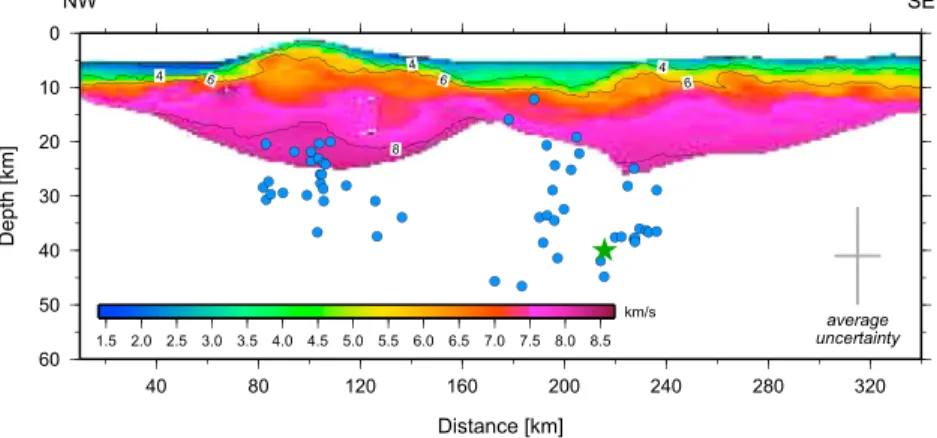
Figure 5.Earthquake hypocentres (dots) obtained with the 3-D velocity model. We show only events recorded with an azimuthal gap<270° and within30 km of the profile A-A⁰(see Figure 2). Hypocenters are projected on the velocity model ofMartinez-Loriente et al.[2014]. The green star marks the 2007M_w= 6.0 Horseshoe earthquake. For comparison with 1-D models see Figure S5.

4.4. Moment Tensor Inversion of the 2007 Horseshoe Earthquake

We used an iterative least squares inversion [e.g.,Kikuchi and Kanamori, 1991] of azimuthally distributed seis- micPandSHwave seismograms from stations located at epicentral distances between 30° and 90° in order to infer the rupture mechanism, depth, and source time function of the 2007 Horseshoe earthquake. Waveforms are corrected for instrument responses to obtain displacement seismograms. The inversion assumes attenua- tion with at* (travel time divided by averageQ) of 1 s forPwaves and 4 s forSHwaves. The Green functions were computed by using a layered source and receiver structures connected by geometric spreading for the AK135 Earth model [Kennett et al., 1995]. At the source region we included a water layer overlying a half space withV_p= 6.0 km/s,V_s= 3.55 km/s andρ= 2.67 g/cm³. The source wasfixed at the epicenter reported byStich et al.[2007]. For the inversion, we used 19Pwaves and 5SHwaves from good-quality waveforms. In addition, we investigated the possibility of more complex rupture behavior, introducing up to three subevents.

4.5. Focal Mechanisms From First Motion Polarities

In local marine earthquake studies, double-couple focal mechanisms are generally retrieved fromPwavefirst motions. In order to improve solutions, we addedfirst motion polarities from waveform data of land stations in Portugal. Unfortunately, all recorded local events were too small to be studied by regional moment tensor inversion. We therefore computed fault plane solutions by using HASH, FOCMEC, and FPFIT algorithms [Hardebeck and Shearer, 2002;Snoke et al., 1984;Reasenberg and Oppenheimer, 1985], not allowing for any polarity error (Figure S4). Here we report only the four focal mechanisms for which the different approaches provided similar solutions (Table 1) and for which polarities from both OBS records and permanent networks were available.

5. Results

Our two deployments provided for thefirst time detailed information on the distribution of microseismicity derived from dense offshore networks. The area was previously studied byGeissler et al.[2010] using offshore seismometers, reporting 36 earthquakes of magnitude Ml 2.2 to 4.8. However, they used a sparse station spa- cing of ~50 km, while our deployments used a station spacing of 5 to 10 km, reducing uncertainties of focal parameters. Further, with 160 local earthquakes our study reported a much larger number of well-located microearthquakes and placed detailed constraint on a number of active tectonic features that were not included in the catalogue ofGeissler et al.[2010], including the Gorringe Bank and the Southwest Iberian Margin (SWIM) lineaments to the north of Coral Patch Ridge. Further, our study benefitted from recently published seismic refraction data [Sallarès et al., 2013;Martinez-Loriente et al., 2014], providing detailed constraints on the seismic velocity structure of the tectonically active area to the southwest of Portugal, minimizing bias caused by inappropriate velocity models.

5.1. Distribution of Microseismicity Using 1-D Velocity Models 5.1.1. The Horseshoe Abyssal Plain (HAP) Deployment

We detected and located 82 local earthquakes with good station coverage and at close distances to the net- work. Most earthquakes ruptured within the Horseshoe Abyssal Plain and in the vicinity of the Horseshoe Fault. In general, the number ofSonset readings on the OBS records was rather small and the waveforms were rather complex (Figure 3a). Complex secondary arrivals might be due to internal reflections within the 5 km thick sedimentary layer. Therefore, initially we located events by usingPwaves only. Later, we used

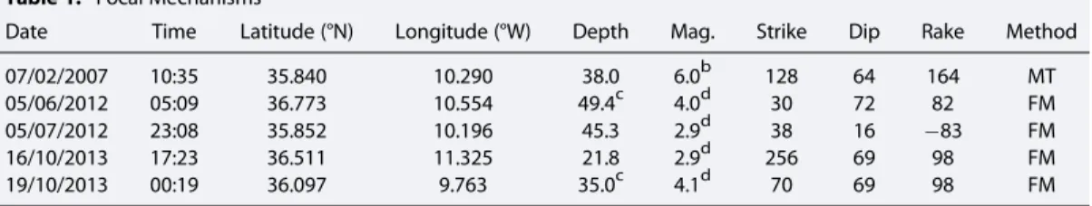
Table 1. Focal Mechanisms^a

Date Time Latitude (°N) Longitude (°W) Depth Mag. Strike Dip Rake Method

07/02/2007 10:35 35.840 10.290 38.0 6.0^b 128 64 164 MT

05/06/2012 05:09 36.773 10.554 49.4^c 4.0^d 30 72 82 FM

05/07/2012 23:08 35.852 10.196 45.3 2.9^d 38 16 83 FM

16/10/2013 17:23 36.511 11.325 21.8 2.9^d 256 69 98 FM

19/10/2013 00:19 36.097 9.763 35.0^c 4.1^d 70 69 98 FM

aMT: Teleseismic moment tensor inversion; FM:first motion polarities, including land stations.

bMoment magnitude (M_w).

cLocated with GAP>270°.

dLocal magnitude (Ml).

bothPandSarrivals. Overall, focal parameters were very similar, but some events under the HAP were very shallow when usingPwaves only for the location. After introducingSwaves, the events moved to basement depths, about 5 km below the seafloor. Deeper events showed nearly identical depth distributions when using onlyPwaves and bothPandSwaves (Figure S5).

The largest event within the HAP deployment (GAP<180°) had a local magnitude of 3.3 and occurred on 5 July 2012 at ~40 km depth. Figure 4 shows waveforms of this event recorded by the hydrophone. The arrival times are plotted as a function of hypocentral distance, indicating apparent velocities of 8 km/s, and thus supporting the inference that the event occurred in the mantle. Note that this inference is independent from the epicenter. All located earthquakes ruptured below 10 km and hence within the igneous basement or deeper (Figures 5 and S5).

Most earthquakes occurred within the mantle at 25 to 40 km depth, with no evidence for earthquakes below

~45 km. Structurally, earthquake to the west of the Horseshoe Fault occurred within unroofed continental mantle and to the east within oceanic lithosphere (Figure S3) [Sallarés et al., 2011;Martinez-Loriente et al., 2014].

A second cluster of earthquake activity occurred at the termination of the Cabo Sao Vicente Canyon, to the SW of Cabo Sao Vicente. These events had a reasonably small azimuthal gap when considering the permanent onshore network in Portugal (Figure S1).

Two other rather strong earthquakes with Ml = 3.9 and 4.1 struck the southeastern edge of the Gorringe Bank on 5 June 2012. The larger magnitude 4.1 event was the strongest earthquake recorded during network operation. Its thrust-type focal mechanism suggests shortening in the direction of NW-SE convergence (Table 1 and Figure 2).

Earthquake epicenters correlate very weakly with fault traces mapped either by bathymetric data (like the SWIM faults; Figure S1) or by seismic reflection data. Thus, neither the NE-SW striking Horseshoe Fault is out- lined by increased levels of seismicity nor are the WNW-ESE striking SWIM lineaments highlighted as a band of significant seismicity. However, some earthquakes that occurred outside of the network, in the vicinity of the Coral Patch Ridge (CPR), may indicate activity along the SWIM lineaments. Unfortunately, these events occurred outside of the network, and therefore, we could not robustly compute their hypocenters.

5.1.2. The Gorringe Bank (GB) Deployment

Seismicity rate was very low at the GB and only about 50 local earthquakes could be detected by the local OBS deployment. In particular, we detected only four new events with respect to the Portuguese seismic cat- alogue. The largest event had a magnitude of Ml = 3.6 and occurred while the seismic network was recovered, on 25 March 2014. Most earthquakes occurred below the Gorringe Bank. In addition, sparse events occurred beneath the HAP, near the termination of the Sao Vicente Canyon, and in the vicinity of the SWIM lineaments to the north of Coral Patch Ridge (Figure S2).

Like for the HAP network, we initially located events by usingPwaves only. Later, we includedSwaves.

Overall,Swaves are much better developed for earthquakes recorded at the Gorringe Bank than at the HAP (Figure 3b), and therefore, the number of availableSpicks is higher. Similar depth estimates were obtained both usingPwaves only and using bothPandSwaves. Events occurred at depths of 15 to 30 km, a bit shallower than those observed in the HAP (Figures 5 and S5). Events showed rather fast apparent velocities, similar to those in the HAP. The distribution of seismicity, both in map view and in cross section, does not show any clear relation to fault structures.

5.2. Distribution of Microseismicity Using a Quasi-3-D Model

We used the quasi-3-D model in order to locate all events detected by the two networks. In total, about 120 local earthquakes were available. Overall, the results are very similar to those obtained with a 1-D model. Thus, we confirmed that earthquakes in the HAP occurred at greater depth than at the GB, with earthquakes occurring at 18 to 36 km below Gorringe Bank and at 10 to 47 km below the Horseshoe Abyssal Plain, respectively (Figure 5). In addition, a large number of earthquakes clustered to the north of Coral Patch Ridge, indicating active fault motion (Figure 2) along the SWIM lineament [Zitellini et al., 2009;Martínez-Loriente et al., 2013].

5.3. Focal Mechanism and Centroid Depth of the 2007 Horseshoe Earthquake

The teleseismic waveform inversion suggests that the 12 February 2007 earthquake had an oblique dip-slip motion with a strike = 129°, dip = 64°, and rake = 165°, with slip occurring below 30 km and with a bestfit (misfit of 0.48) centroid depth of 38 km (Figure 6). Thus, the mechanism is similar to that obtained by regional

moment tensor inversion, which results in a strike = 128°, dip = 46°, and rake = 138° and a depth of 39 km [Custódio et al., 2012]. The dip obtained from teleseismic data in this study is slightly steeper than that reported byCustódio et al.[2012]. The best depth estimates indicate that most of the seismic moment was released at mantle depths, well below the volume sampled by seismic refraction data [Martinez-Loriente et al., 2014]. The source time function indicates a rather short rupture duration of 2 s and a moment magni- tude ofM_w= 6.

However, waveforms recorded at stations in North and South America showed a precursor that is notfitted when inverting for a single double-couple source (Figures 6 and 7). We increased rupture complexity by introducing a number of subevents, thus improving waveformfit (misfit of 0.38). Introducing up to three subevents yielded a sequence of events with similar rupture mechanisms, including a small thrust-type pre- cursor just before the main shock and a third event with moderate energy. The total moment of the three subevents wasM_w= 6.1 (Figure 7).

6. Discussion

6.1. Distribution of Seismicity

The Gulf of Cadiz and adjacent domains to the SW of Portugal are interpreted as a diffusive plate boundary, where seismicity and deformation are distributed over an ~200 km wide area [e.g., Sartori et al., 1994;

Hayward et al., 1999]. However, the re-analysis of the instrumental earthquake catalogue for western Iberia showed that although this plate boundary is diffuse in that deformation is accommodated along several distributed faults rather than along one long linear plate boundary [e.g.,Hayward et al., 1999;Terrinha et al., 2009;Martínez-Loriente et al., 2013], the seismicity itself is not diffuse but rather collapses into well-defined Figure 6.Waveform inversion of theM_w= 6.0 12 February 2007 Horseshoe Fault earthquake using stations at epicentral distances between 30° and 90°; (a) focal mechanism, (b) source time function, (c) grid search of centroid depth, and (d) waveformfit (black and blue: observed; red: calculated). The best depth estimate of 38 km supports that the event ruptured within the oceanic mantle. Note that observed waveforms plotted in blue indicate stations in South and North America, providing a poor misfit to the onset of modeled waveforms.

clusters and lineations [Zitellini et al., 2001;Custódio et al., 2015;Grevemeyer et al., 2016]. The most seismically active offshore areas are the GB, the HAP, the Sao Vicente Canyon (SVC), and the Mesozoic Algarve margin.

Our OBS networks, supplemented by Portuguese land stations, confirm activity at GB, HAP, and at the southern terminus of the Sao Vicente Canyon. While the GB and SVC present indeed clustered activity, seis- micity in the HAP seems to occur over an ~40 km wide and ~100 km long band that strikes NW-SE (Figure 2).

In addition, some earthquakes, located with the 3-D model, to the east of the networks seem to collapse along faults that run to the north of Coral Patch Ridge (Figure 2).

The observed seismicity pattern might be best explained by the model of Terrinha et al. [2009], who suggest that convergence is accommodated by strain partitioning on WNW-ESE trending dextral steep faults and NE-SW trending thrust faults in the Gulf of Cadiz and Horseshoe Abyssal Plain. Approaching the base of the continental slope, including the SVC, NNE-SSW to N-S westerly dipping thrusts accommodate shortening in an area where wrenching has not been observed [Terrinha et al., 2009].

6.2. Hypocentral Depth

The teleseismic data indicate that the hypocentral depth of the 12 February 2007 Horseshoe Fault earthquake was 382 km, in agreement with previous estimates of 39 km to 40 km derived from regional waveform data [Stich et al., 2007;Custódio et al., 2012]. The teleseismic waveform inversion confirms a rupture plane trending Figure 7.Waveform inversion of the 12 February 2007 Horseshoe Fault earthquake considering up to three subevents and achieving a better waveformfit, most importantly to early onsets observed in north and south America (see text and Figure 6); (a) source time function, (b) mechanisms, and (c) waveformfit (black and blue: observed; red: calculated).

WNW-ESE. Microearthquakes located with the OBS data in the HAP occurred on average at depths of 26.911.8 km (1-D velocity model) or 31.5 km10.5 km (3-D velocity model). Thus, both local earthquakes and the 2007M_w= 6.0 earthquake seem to rupture at similar depth ranges within the mantle. Earthquakes in the GB area occur at a shallower depth of 23.75.7 km (1-D velocity model) or 26.17.2 km (3-D velocity model). Seismic refraction indicates that below 15–20 km, the lithosphere has velocities of>8 km/s both at the HAP [Martinez-Loriente et al., 2014] and at the GB [Sallarès et al., 2013;Martinez-Loriente et al., 2014];

hence, it may correspond to unaltered dry mantle. Besides, the majority of microearthquakes occurred well below the depth sampled by seismic reflection data. Consequently, any relationship between seismicity and mapped faults remains speculative, supporting previous observations based on land data [Custódio et al., 2015]. It might be reasonable to speculate that shallow surface faults imaged by seismic reflection data are splays of deep-seated faults.

The largest instrumentally recorded earthquake in the HAP occurred on 28 February 1969. It had a moment magnitude ofM_w= 7.8 and a focal depth of 21 km [Engdahl and Villaseñor, 2002]. Additional regional events reported in the EHB catalogue [Engdahl et al., 1998] show source depths of 5 to 47 km for the HAP [e.g.,Stich et al., 2005], supporting our estimates. In contrast,Stich et al.[2005] concluded that some earthquakes in the HAP may rupture as deep as 60 km. Their assessment was based on waveform modeling of threeM_w= 3.8 to 5.3 earthquakes recorded in Portugal, Spain, and Morocco.Geissler et al.[2010] reported 36 microearthquakes located with an amphibious network, including OBS. Their depth estimates are systematically deeper than our estimates, clustering at about 50 km depth. However, bothStich et al.[2007] andGeissler et al.[2010]

conducted their analysis before detailed velocity models derived from modern seismic refraction data were available [Sallarès et al., 2013; Martinez-Loriente et al., 2014] and hence used a much thicker crust or continental-type velocity structure with a 16 to 20 km thick crust, which may bias focal parameters.

We emphasize that the locations presented in this article rely on a local velocity structure inferred from seismic refraction and wide-angle data collected in the study area and on a nonlinear hypocentral inversion algorithm [Lomax et al., 2000], which provides more reliable location uncertainties than linearized inversions.

Further, station corrections were calculated and used in order to minimize local site effects. However, all stu- dies support that seismicity is deep seated, clearly occurring in the Earth’s mantle rather than in the crust.

6.3. Focal Depth and Thermal Structure

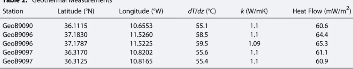
Like the Horseshoe Abyssal Plain, the Iberia Abyssal Plain (IAP) has been classified as a domain of unroofed continental mantle [e.g.,Minshull et al., 2014] that was formed during continental breakup. Heatflow in the IAP is on the order of 46 mW/m²[Louden et al., 1997]. Here we report unpublished heatflow data from the HAP and Tagus Abyssal Plain (Table 2), which show a heatflow of 60 to 65 mW/m², mimicking measure- ments obtained in the vicinity of Cabo Sao Vicente off southwestern Portugal [Grevemeyer et al., 2009]. The reported heatflow data were obtained in 2003 by using a 3 m long violin-bow design heat probe and were analyzed by using the same procedure described byGrevemeyer et al.[2009] to study the Gulf of Cadiz.

Higher heatflow in the HAP and near the GB seems to be a regional feature (Figure S6), with lower heatflow observed to the north in the IAP [Louden et al., 1997] and to the east in the Gulf of Cadiz [Grevemeyer et al., 2009]. The distributed deformation of the domain to the east of Gibraltar [Sartori et al., 1994;Terrinha et al., 2009; Custódio et al., 2015] might be analogous to the intraplate deformation observed in the Indian Ocean [e.g.,Wiens et al., 1985]. Like the HAP, the Central Indian Ocean is characterized by anomalously high heatflow.Delescluse and Chamot-Rooke[2008] suggested that the observed spatial correlation between high heatflow and active thrust faulting supports exothermic heat generated by serpentinization. Given that

Table 2. Geothermal Measurements

Station Latitude (°N) Longitude (°W) dT/dz(°C) k(W/mK) Heat Flow (mW/m²)

GeoB9090 36.1115 10.6553 55.1 1.1 60.6

GeoB9096 37.1830 11.5260 58.5 1.1 64.4

GeoB9096 37.1787 11.5225 59.5 1.09 65.3

GeoB9097 36.3170 10.8202 55.6 1.1 61.1

GeoB9097 36.3125 10.8165 55.4 1.1 60.9

serpentinization has been observed throughout the HAP and GB, it is plau- sible to admit that serpentinization does indeed cause higher heatflow in the vicinity of the Gorringe Bank.

The maximum depth of faulting and hence earthquake nucleation has been previously related to tempera- ture. In the oceanic mantle, brittle deformation is a common feature and generally restricted to tempera- tures <600°C [e.g., McKenzie et al., 2005; Craig et al., 2014]. Thus, near mid-ocean ridges seismicity is con- fined to crustal levels [e.g., Grevemeyer et al., 2013], whereas the brittle deformation of mature ocea- nic lithosphere may extend several tens of kilometres into the mantle [Lefeldt et al., 2009;Craig et al., 2014].

In order to study the temperature structure as a function of depth, we calculated a suite of geotherms for a layered structure of (1) sediment and (2) serpentinized mantle with a thickness of 4 and 14 km, respec- tively, and (3) dry mantle below. The sedimentary thickness of 5 km has been assessed by using reflection seismic data from the HAP [Rovere et al., 2004;Martínez-Loriente et al., 2013] and the thickness of the serpentinized domain has been approxi- mated by the depth to the 8 km/s velocity isocontour below the HAP [Sallarès et al., 2013]. Below, a domain of dry mantle with a constant heatflow at its base is considered. The conductive geotherm in a horizontally stratified subsurface is calculated by solving the steady state heatflow equation

d²T zð Þ

dz² ¼Að Þz k zð Þ

in each layer withAas heat production andkas thermal conductivity. All layers are characterized by isotropic and homogeneous thermal properties and heat production. Temperature and heatflow are continuous at layer boundaries. The surface (z= 0) is kept atT₀= 0, and at the bottom layer a basal heatflow is prescribed.

In order to assign uncertainties to the thermal properties and temperature structure as a function of depth, each parameter was allowed to vary randomly within preset boundaries in each layer. For each random combination of parameters a geotherm was calculated and surface heatflow and temperature as a function of depth were averaged.

Our reference site was the Iberia Abyssal Plain. The observed surface heatflow of 46 mW/m²[Louden et al., 1997]

was modeled by using thermal conductivitieskfor sediment, serpentinized mante, and mantle of 2.0, 3.0, and 3.3 W/mK and a heat productionAof 0, 0.01, and 0.5μW/m³, respectively [e.g.,Louden et al., 1997;McKenzie et al., 2005;Jiménez-Munt et al., 2010]. In this model, the temperature at 45 km below seafloor (or at ~50 km below sea level with 5 km of water) is 600°C, when considering a basal heatflow of 30 mW/m²(Figures 8 and S7a). Varying the basal heatflow from 35 to 25 mW/m²suggests uncertainties for the temperature at 45 km below seafloor of48.8°C.

To obtain an increased surface heatflow, as sampled in the HAP, it is unlikely that the basal heatflow is increased, too, as it would affect adjacent areas, like the Gulf of Cadiz, which is characterized by low heatflow of<50 mW/m² [Grevemeyer et al., 2009]. We therefore consider either (i) exothermic heat generated by Figure 8.(left) Earthquake depth distribution of the well-located micro-

earthquakes and (right) results from thermal modeling; black line indicates reference model for the Iberia Abyssal Plain setting (surface heatflow of 46 mW/m²); red line indicates model with high radiogenic heat production in sediments; blue line indicates“serpentinization model.”The blue and red models provide the observed surface heatflow of 61 mW/m². The broken lines mark the depths of the 600°C isotherme. A temperature of 600°C is generally expected to mark the seismic-to-aseismic transition [e.g.,McKenzie et al., 2005].

deformation and serpentinization or (ii) increased radiogenic heat production in sediments deposited in the HAP as potential sources.

Thefirst scenario is based on the serpentinization model ofDelescluse and Chamot-Rooke [2008] for the Central Indian Ocean (Figures 8 and S7b). In order to simulate exothermic heat generation caused by hydra- tion of dry mantle to serpentine, we introduce an artificial additional heat production of 1.5μW/m³in the sec- ond layer (the full set of parameters is given in Figure S7). As a result, we were able to generate the observed surface heatflow of 61 mW/m², indicating an increase in mantle temperature reaching 65549°C at 45 km below seafloor or about 600°C at 40 km below seafloor.

In the second case (Figures 8 and S7c), keeping the original reference model, but increasing the radiogenic heat production in the sedimentary layer to 4μW/m³, we were able to produce the observed surface heat flow. The temperature at a depth of 45 km below seafloor is 61648.8°C and hence has increased with respect to the reference model only by a few degrees. However, the second scenario is less likely, because if eroded from the Iberian continent, it would be reasonable to assume that the same type of sedimentfills all basins adjacent to Iberia, including the IAP, where heatflow is much lower. Further, radiogenic heat pro- duction in Iberia is highest for granites, ranging from 2.5 to 3.7μW/ m³, while metasediments and basic rocks have a lower heat production, ranging from 1 to 2.5μW/m³[Fernàndez et al., 1998]. Consequently, deposits of weathered rocks containing a suite of different rock types will have a heat production that will be well below 4μW/m³. We therefore conclude that the exothermic serpentinization model provides the bestfit to the observed features, suggesting that rupture is limited to the upper 40 km of the lithosphere and hence down to<45 km below sea level. This assessment correlates well with the observed depth distribution of micro- earthquakes and centroid of the 2007M_w= 6.0 earthquake. However, all models, including the reference model of much lower surface heatflow, suggest that seismogenic behavior will inherently be related to the upper 455 km of the lithosphere. Therefore, previous depth estimates of seismogenic rupture down 60 km [Stich et al., 2007; Geissler et al., 2010] are not supported by the thermal state of the lithosphere derived from our model.

6.4. Hazard Potential

Seismic moment is defined byM₀=μA D, whereμis the shear moduli of the rocks involved in the earth- quake, A is the size of the rupture plane, and D is the average displacement [e.g., Kanamori, 1977].

Rupturing at mantle depth may support rather large shear moduli of 50 [Ammon et al., 2008] to 70 MPa [Stich et al., 2007]. Great earthquakes of magnitudeM_w= 8.2 to 8.7 rupturing the oceanic lithosphere may cause>15 m [Lay et al., 2009] and probably up to 35 m [Yue et al., 2012] of slip. A steeply dipping fault of

~64°, as indicated by the 2007 Horseshoe earthquake, would support a down-dip width of ~45 to 50 km. A shallower dip of the fault [Fukao, 1973;Custódio et al., 2012] would support a rupture plane with a downdip width of up to 60 km. Thus, considering a 60 km by 200 km wide fault, an average slip of 20 m and a shear moduli of 50 GPa [Ammon et al., 2008] could cause a seismic moment of 1.2 · 10²²Nm and hence aM_w= 8.7 earthquake. Consequently, a fault with approximately the length of the Gorringe Bank could cause a 1755 Lisbon-type earthquake and associated tsunami. Shorter faults, like the ~120 km long Horseshoe Fault [Zitellini et al., 2009], may not provide enough moment to cause a great earthquake. However, the great Lisbon earthquake may have been a compound event, triggering adjacent faults [e.g.,Vilanova et al., 2003]. A similar behavior was observed during the 2012M_w= 8.7 Indian Ocean intraplate earthquake [Yue et al., 2012], suggesting that earthquakes in cold mantle lithosphere have indeed the potential to pose significant hazards.

6.5. Tectonic Implications

The formation of the Gorringe Bank has been related to Miocene tectonics [e.g.,Tortella et al., 1997;Zitellini et al., 2004], including uplift and overthrusting of the HAP and GB onto the Tagus Abyssal Plain. It has now been recognized that shortening of 20 to 50 km [Galindo-Zaldívar et al., 2003;Jiménez-Munt et al., 2010;

Hayward et al., 1999] occurred in a domain of unroofed mantle as inferred by seismic data [Pinheiro et al., 1992;Rovere et al., 2004;Martinez-Loriente et al., 2014]. In contrast, scenarios of shortening generally consider a domain composed of oceanic crust and faulting at a depth of 5 to 15 km below seafloor [e.g.,Jiménez-Munt et al., 2010; Duarte et al., 2013]. However, basal faults have never been seismically imaged but were envisioned based on conceptual models. It might be important to emphasize that these scenarios envision faulting at a much shallower depth levels than revealed by our study. Furthermore, the great depth of

faulting of >20 km under the GB may not support the development of a shallow dipping subduction megathrust [e.g.,Duarte et al., 2013]. Rather, we favor the interpretation that a block of cold ~120 Ma old continental mantle is sandwiched between two domains of mature oceanic lithosphere, namely, Eurasia in the northwest and Africa in the southwest, and deformed during convergence.

7. Conclusions

Two networks of ocean bottom seismometers were deployed to monitor microseismicity in the Horseshoe Abyssal Plain and at the Gorringe Bank. Both regions may encompass the fault that generated the Great Lisbon earthquake of 1755. Our results suggest the following:

1. Most earthquakes were located at>20 km depth in the upper mantle of domains previously interpreted as unroofed continental mantle and oceanic mantle.

2. Maximum depth of faulting, inferred both using 1-D and 3-D velocity models, is ~45 km.

3. Thermal modeling suggest that temperatures of 600°C are reached at approximately 45 km depth and hence explains the lack of microearthquakes below 45 km, suggesting that previous estimates of source depths extending down to 60 km depth [Stich et al., 2007; Geissler et al., 2010] might be too deep.

4. Microearthquakes generally occur at depths greater than geologically and reflection seismically mapped faults. Thus, fault systems imaged in the bathymetry and seismic reflection data may splay out from deep- seated faults.

5. Focal depth seems to increase from 20–35 km (mean of 26.17.2 km) at the Gorringe Bank to 15–45 km (mean 31.5 km10.5 km) under the Horseshoe Abyssal Plain.

6. The focal parameters of microearthquakes, waveform inversion of the 2007M_w= 6.0 Horseshoe earth- quake, and thermal models suggest that an approximately 200 km long fault in the vicinity of the Horseshoe Abyssal Plain could support a M_w= 8.7 1755 Lisbon-type earthquake in cold lithospheric mantle.

7. We suggest that the distributed deformation and seismicity of the Horseshoe Abyssal Plain and Gorringe Bank are related to the African-Eurasian convergence and deformation of a domain of unroofed Cretaceous continental mantle sandwiched between two domains of>120 Ma old oceanic lithosphere.

We do notfind in the microseismicity data evidence for a developing subduction zone.

References

Ammon, C. J., H. Kanamori, and T. Lay (2008), A great earthquake doublet and seismic stress transfer cycle in the central Kuril islands,Nature, 451, 561–566, doi:10.1038/nature06521.

Auzende, J. M., et al. (1984), Intraoceanic tectonism on the Gorringe Bank: Observations by submersible, inOphiolites and Oceanic Lithosphere, edited by I. G. Gass, S. J. Lippard, and A. W. Shelton,Geol. Soc. London, Spec. Publ., 13, 113–120.

Baptista, M. A., J. M. Miranda, R. Omira, and C. Antunes (2011), Potential inundation of Lisbon downtown by a 1755-like tsunami,Nat. Hazards Earth Syst. Sci.,11, 3319–3326.

Barkan, R., U. Ten Brink, and J. Lin (2009), Farfield tsunami simulations of the 1755 Lisbon earthquake: Implications for tsunami hazard to the U.S. East Coast and the Caribbean,Mar. Geol.,264, 109–122.

Bird, P. (2003), An updated digital model of plate boundaries,Geochem. Geophys. Geosyst.,4(3), 1027, doi:10.1029/2001GC000252.

Craig, T. J., A. Copley, and J. Jackson (2014), A reassessment of outer-rise seismicity and its implications for the mechanics of oceanic lithosphere,Geophys. J. Int.,197, 63–89, doi:10.1093/gji/ggu013.

Custódio, S., S. Cesca, and S. Heimann (2012), Fast kinematic waveform inversion and robustness analysis: application to the 2007 Mw 5.9 Horseshoe Abyssal Plain Earthquake Offshore Southwest Iberia,Bull. Seismol. Soc. Am.,102(1), 361–376.

Custódio, S., N. A. Dias, F. Carrilho, E. Góngora, I. Rio, C. Marreiros, I. Morais, P. Alves, and L. Matias (2015), Earthquakes in western Iberia: Improving the understanding of lithospheric deformation in a slowly deforming region,Geophys. J. Int.,203, 127–145, doi:10.1093/gji/ggv285.

Delescluse, M., and N. Chamot-Rooke (2008), Serpentinization pulse in the actively deforming Central Indian Basin,Earth Planet. Sci. Lett.,276, 140–151.

DeMets, C., R. G. Gordon, and D. F. Argus (2010), Geologically current plate motions,Geophys. J. Int.,181, 1–80.

Duarte, J. C., F. M. Rosas, P. Terrinha, W. P. Schellart, D. Boutelier, M.-A. Gutscher, and A. Ribeiro (2013), Are subduction zones invading the Atlantic? Evidence from the southwest Iberia margin,Geology,41(8), 839–842.

Engdahl, R., R. van der Hilst, and R. Buland (1998), Global teleseismic earthquake relocation with improved traveltimes and procedures for depth determination,Bull. Seismol. Soc. Am.,88, 722–743.

Engdahl, E. R., and A. Villaseñor (2002), Global Seismicity: 1900–1999, inInternational Handbook of Earthquake and Engineering Seismology, Part A, edited by W. H. K. Lee et al., chap. 41, pp. 665–690, Academic Press.

Féraud, G., D. York, C. Mével, G. Cornen, C. M. Hall, and J. M. Auzende (1986), Additional⁴⁰Ar/³⁹Ar dating of the basement and the alkaline volcanism of Gorringe Bank (Atlantic Ocean),Earth Planet. Sci. Lett.,79(3–4), 255–269.

Fernàndez, M., I. Marzán, A. Correia, and E. Ramalho (1998), Heatflow, heat production, and lithospheric thermal regime in the Iberian Peninsula,Tectonophysics,291, 29–53, doi:10.1016/S0040-1951(98)00029-8.

Fukao, Y. (1973), Thrust faulting at a lithospheric plate boundary: The Portugal earthquake of 1969,Earth Planet. Sci. Lett.,18, 205–216.

Acknowledgments

This study was funded by the German Science Foundation (DFG grant GR1964/15-1), GEOMAR’s OCEANS pro- gram, and benefitted from COST Action ES1301“FLOWS.”We like to thank Captain’s Bernhard Windscheid and Matthias Günther and their crews of R/V Poseidoncruises POS430, POS440, POS460, and POS467 for excellent sea- going support. We are grateful to Kathrin Lieser, Carlos Corela, Stefan Möller, Sven Schippkus, Patrick Schröder, and Klaus-Peter Steffen for their technical assistance in operating ocean bottom seismometers. Seismic data were analyzed by using SEISAN [Havskov and Ottemöller, 2000], and figures were produced by using the Generic Mapping Tools software [Wessel and Smith, 1998]. This work included data from the II, IU, GT, GE, and CU seismic networks obtained from the IRIS data center (https://doi.org/

doi:10.7914/SN/II; https://doi.org/

doi:10.7914/SN/IU; https://doi.org/

doi:10.14470/TR560404; https://doi.org/

doi:10.7914/SN/GT). Travel time data for the land stations used in the 1-D loca- tion procedure were from the ISC online catalogue (http://www.isc.ac.uk). We thank two anonymous referees and the Associate Editor for constructive reviews that improved the manuscript.

Seismological data are available on request from thefirst author.

Galindo-Zaldívar, J., A. Maldonado, and A. A. Schreider (2003), Gorringe Ridge gravity and magnetic anomalies are compatible with thrusting at crustal scale,Geophys. J. Int.,153, 586–594, doi:10.1046/j.1365-246X.2003.01922.x.

Geissler, W. H., et al. (2010), Focal mechanisms for sub-crustal earthquakes in the Gulf of Cadiz from a dense OBS deployment,Geophys. Res.

Lett.,37, L18309, doi:10.1029/2010GL044289.

Girardeau, J., G. Cornen, M. O. Beslier, B. Le Gall, C. Monnier, P. Agrinier, G. Dubuisson, L. Pinheiro, A. Ribeiro, and A. Whitechurch (1998), Extensional tectonics in the Gorringe Bank Rocks, eastern Atlantic Ocean: Evidence of an oceanic ultra-slow mantellic accreting centre, Terra Nova,10(6), 330–336.

Grandin, R., J. F. Borges, M. Bezzeghoud, B. Caldeira, and F. Carrilho (2007), Simulations of strong ground motion in SW Iberia for the 1969 February 20 (Ms = 8.0) and the 1755 November 1 (M ~ 8.5) earthquakes–II. Strong ground motion simulations,Geophys. J. Int.,171, 807–822.

Grevemeyer, I. (2015), RV POSEIDON Cruise Report POS430, POS440, POS460 and POS467—Seismic hazards to the southwest of Portugal;

GEOMAR Report, N.Ser. 024 GEOMAR Helmholtz-Zentrum für Ozeanforschung Kiel, Kiel, 43 pp., doi:10.3289/GEOMAR_REP_NS_24_2015.

Grevemeyer, I., N. Kaul, and A. Kopf (2009), Heatflow anomalies in the Gulf of Cadiz and off Cape San Vincente,Portugal. Mar. Petrol. Geol.,26, 795–804, doi:10.1016/j.marpetgeo.2008.08.006.

Grevemeyer, I., T. J. Reston, and S. Moeller (2013), Microseismicity of the Mid-Atlantic Ridge at 7°S-8°15⁰S and at the Logatchev Massif oceanic core complex at 14°40⁰N-14°50⁰N,Geochem. Geophys. Geosyst.,14, 3532–3554, doi:10.1002/ggge.20179.

Grevemeyer, I., E. Gràcia, A. Villaseñor, W. Leuchters, and A. B. Watts (2015), Seismicity and active tectonics in the Alboran Sea, Western Mediterranean: Constraints from an offshore-onshore seismological network and swath bathymetry data,J. Geophys. Res. Solid Earth,120, 8348–8365, doi:10.1002/2015JB012073.

Grevemeyer, I., L. Matias, and S. Silva (2016), Mantle earthquakes beneath the South Iberia continental margin and Gulf of Cadiz— Constraints from an onshore-offshore seismological network,J. Geodynamics,99, 39–50, doi:10.1016/j.jog.2016.06.001.

Gutscher, M. A., et al. (2012), The Gibraltar subduction: A decade of new geophysical data,Tectonophysics,574–575, 72–91, doi:10.1016/j.

tecto.2012.08.038.

Hardebeck, J. L., and P. M. Shearer (2002), A new method for determiningfirst-motion focal mechanisms,Bull. Seismol. Soc. Am.,92, 2264–2276, doi:10.1785/0120010200.

Havskov, J., and L. Ottemöller (2000), SEISAN earthquake analysis software,Seismol. Res. Lett.,70, 532–534.

Hayward, N., A. B. Watts, G. K. Westbrook, and J. S. Collier (1999), A seismic reflection and GLORIA study of compressional deformation in the Gorringe Bank region, eastern North Atlantic,Geophys. J. Int.,138(3), 831–850.

Hutton, L. K., and D. M. Boore (1987), The Ml scale in Southern California,Bull. Seismol. Soc. Am.,77(6), 2074–2094.

Jiménez-Munt, I., M. Fernàndez, J. Vergés, J. C. Afonso, D. Garcia-Castellanos, and J. Fullea (2010), Lithospheric structure of the Gorringe Bank:

Insights into its origin and tectonic evolution,Tectonics,29, TC5019, doi:10.1029/2009TC002458.

Johnston, A. (1996), Seismic moment assessment of earthquakes in stable continental regions—III. New Madrid, 1811–1812, Charleston 1886 and Lisbon 1755,Geophys. J. Int.,126, 314–344.

Kanamori, H. (1977), The energy release of great earthquakes,J. Geophys. Res.,82, 2981–2987, doi:10.1029/JB082i020p02981.

Kennett, B. L. N., E. R. Engdahl, and R. Buland (1995), Constraints on seismic velocities in the Earth from traveltimes,Geophys. J. Int.,122, 108–124, doi:10.1111/j.1365-246X.1995.tb03540.x.

Kikuchi, M., and H. Kanamori (1991), Inversion of complex body waves-III,Bull. Seismol. Soc. Am.,81(6), 2335–2350.

Lay, T., H. Kanamori, C. J. Ammon, A. R. Hutko, K. Furlong, and L. Rivera (2009), The 2006–2007 Kuril Islands great earthquake sequence, J. Geophys. Res.,114, B11308, doi:10.1029/2008JB006280.

Lefeldt, M., I. Grevemeyer, J. Gossler, and J. Bialas (2009), Intraplate seismicity and related mantle hydration at the Nicaraguan trench outer rise,Geophys. J. Int.,178, 742–752, doi:10.1111/j.1365-246X.2009.04167.x.

Louden, K. E., J.-C. Sibuet, and F. Harmegnies (1997), Variations in heatflow across the ocean-continent transitioln in the Iberia abyssal plain, Earth Planet. Sci. Lett.,151, 233–254.

Lomax, A., A. J. Virieux, P. Volant, and C. Berge (2000), Probabilistic earthquake location in 3D and layered models: Introduction of a Metropolis-Gibbs method and comparison with linear locations, inAdvances in Seismic Event Location, edited by C. H. Thurber and N.

Rabinowitz, pp. 101–134, Kluwer Acad., Amsterdam.

Martinez-Solares, J. M., A. Lopez, and J. Mezcua (1979), Isoseismal map of the 1755 Lisbon earthquake obtained from Spanish data, Tectonophysics,53, 301–313.

Martínez-Loriente, S., et al. (2013), Active deformation in old oceanic lithosphere and significance for earthquake hazard: Seismic imaging of the Coral Patch Ridge area and neighboring abyssal plains (SW Iberian Margin),Geochem. Geophys. Geosyst.,14, 2206–2231, doi:10.1002/

ggge.20173.

Martinez-Loriente, S., et al. (2014), Seismic and gravity constraints on the nature of the basement in the Africa-Eurasia plate boundary: New insights for the geodynamic evolution of the SW Iberian margin,J. Geophys. Res. Solid Earth,119, 127–149, doi:10.1002/2013JB010476.

McKenzie, D., J. A. Jackson, and K. Priestley (2005), Thermal structure of oceanic and continental lithosphere,Earth Planet. Sci. Lett.,233, 337–349, doi:10.1016/j.epsl2005.02.005.

Minshull, T. A., S. M. Dean, and R. B. Whitmarsh (2014), The peridotite ridge province in the southern Iberia Abyssal Plain: Seismic constraints revisited,J. Geophys. Res. Solid Earth,119, 1580–1598, doi:10.1002/2014JB011011.

Müller, R. D., M. Sdrolias, C. Gaina, and W. R. Roest (2008), Age spreading rates and spreading asymmetry of the world’s ocean crust,Geochem.

Geophys. Geosyst.,9, Q04006, doi:10.1029/2007GC001743.

Pinheiro, L. M., R. B. Whitmarsh, and P. R. Miles (1992), The ocean-continent boundary off the western continental margin of Iberia-II. Crustal structure in the Tagus Abyssal Plain,Geophys. J. Int.,109, 106–124.

Podvin, P., and L. Lecomte (1991), Finite difference computation of traveltimes in very contrasted velocity models: A massively parallel approach and its associated tools,Geophys. J. Int.,105, 271–284, doi:10.1111/j.1365-246X.1991.tb03461.x.

Purdy, G. M. (1975), The eastern end of the Azores-Gibraltar plate boundary,Geophys. J. Roy. Astron. Soc.,43, 123–150.

Reasenberg, P., and D. Oppenheimer (1985), FPFIT, FPPLOT and FPPAGE: Fortran computer programs for calculating and displaying earthquake fault-plane solutions, U.S. Geol. Surv. Open File Rep., 85–739. [Available at https://pubs.usgs.gov/of/1985/0739/report.pdf.]

Richter, C. F. (1935), An instrumental earthquake magnitude scale,Bull. Seismol. Soc. Am.,25, 1–32.

Rovere, M., C. R. Ranero, R. Sartori, L. Torelli, and N. Zitellini (2004), Seismic images and magnetic signature of Late Jurassic to Early Cretaceous Africa-Eurasia plate boundary off SW Iberia,Geophys. J. Int.,158, 554–568.

Ryan, W. B. R., K. J. Hsü, M. B. Cita, P. Dumitrica, J. Lort, W. Maync, W. D. Nesteroff, G. Pautot, H. Stradner, and F. C. Wezel (1973), Site 120, in Initial Reports of the Deep Sea Drilling Project, vol. XIII, edited by A. G. Kaneps, pp. 19–41, U.S. Gov. Print. Off., Washington, D. C.

Sallarés, V., et al. (2011), Seismic evidence for the presence of Jurassic oceanic crust in the central Gulf of Cadiz (SW Iberia margin),Earth Plant.

Sci. Lett.,311, 112–123, doi:10.1016/j.epsl.2011.09.003.