Chiral perturbation theory for generalized parton distributions and baryon distribution amplitudes

(1)

Chiral perturbation theory for generalized parton distributions and

baryon distribution amplitudes

DISSERTATION

ZUR ERLANGUNG DES DOKTORGRADES DER NATURWISSENSCHAFTEN (DR. RER. NAT.)

DER FAKULT ÄT F ÜR PHYSIK DER UNIVERSIT ÄT REGENSBURG

vorgelegt von Philipp Wein

aus Regensburg

im Jahr 2016

(2)

Pr¨ufungsausschuss:

Vorsitzender: Prof. Dr. Josef Zweck 1. Gutachter: Prof. Dr. Andreas Sch¨afer 2. Gutachter: Prof. Dr. Vladimir M. Braun weiterer Pr¨ufer: Prof. Dr. Ferdinand Evers

(3)

Abstract

In this thesis we apply low-energy effective field theory to the first moments of generalized parton distributions and to baryon distribution amplitudes, which are both highly relevant for the parametrization of the nonperturbative part in hard processes. These quantities yield complementary information on hadron structure, since the former treat hadrons as a whole and, thus, give information about the (angular) momentum carried by an entire parton species on average, while the latter parametrize the momentum distribution within an individual Fock state. By performing one-loop calculations within covariant baryon chiral perturbation theory, we obtain sensible parametrizations of the quark mass dependence that are ideally suited for the subsequent analysis of lattice QCD data.

(4)

(5)

CHAPTER 1 Introduction

Aside from gravitational effects, the dynamics of elementary particles are described by the Stan- dard Model of particle physics, which comprises electromagnetic, weak and strong interactions mediated by gauge bosons. Electromagnetic and weak effects are, actually, remnants of an underlying unified electroweak theory [1–3], whose spontaneous breaking via the Higgs mechanism [4] gives rise to one massless gauge boson (the photon), which is the gauge boson of quantum electrodynamics (QED), and three massive gauge bosons (W^± andZ⁰), the exchange of which generates the weak force. The strong interaction due to gluon exchange is described by quantum chromodynamics (QCD), which is a Yang–Mills theory [5], i.e., a non-Abelian gauge theory, based on SU(3) gauge symmetry. The corresponding conserved charges are called colors:

red, green and blue. In contrast to the Abelian case also the agent of the interaction itself is a color-charge carrier, which leads to gluon self-interaction via the three- and four-gluon vertices.

The probably most important consequence of this behavior is that the beta function, which de- scribes the running of the coupling constant, can be negative depending on the number of colors Nc and flavors Nf. In particular forNc = 3 the one-loop beta function is negative as long as Nf ≤16 which is the case for QCD, whereNf= 6. Therefore, the strong coupling decreases with increasing four-momentum squared allowing for a perturbative treatment of QCD effects, and, eventually, leads to the asymptotic freedom of quarks and gluons. However, to a large extent the complexity and richness of QCD effects is a consequence of its strong coupling at low energies, where the opposite is the case: the coupling becomes large, denying a perturbative treatment, and the microscopic degrees of freedom (quarks and gluons) are confined to directly observable, colorless hadrons. Even very hard processes with large momentum transfer and relevant distances much smaller than the size of a hadron are influenced by the low-scale dynamics, since all measurements take place after hadronization.

The disentanglement of the short and long range contributions to hard processes is the basic concept behind QCD factorization [6–10], where one rewrites the cross section (in case of inclusive processes) or the scattering amplitude (in case of exclusive reactions) as a convolution of a hard

(10)

scattering kernel and a soft part parametrizing the low-energy dynamics. The process-dependent hard scattering part is accessible by perturbation theory in the strong couplingαsusing the usual diagrammatic techniques. The soft part consists of universal, process-independent functions that resolve the inner hadron structure and are intrinsically nonperturbative quantities. Both the hard and the soft parts depend on the factorization scale. The scale dependence is determined by evolution equations. The most prominent example are the DGLAP equations [11–13], which govern the evolution of parton distribution functions (PDFs) relevant in inclusive deep inelastic scattering (DIS). The exact physical cross section has to be independent of the factorization scale. However, in practice one finds that the perturbative expansion is most efficient if one chooses a factorization scale of the order of the large momentum scale of the process (cf., e.g., ref. [14]).

The functions which parametrize the nonperturbative part of the scattering in different experimental setups provide us with manifold information about the internal hadron structure. For instance, ordinary form factors (FFs) are relevant in elastic scattering processes (e.g.,e⁻p→e⁻p) and encode information about the charge distribution. In contrast, the PDFs mentioned above are needed in inclusive deep inelastic reactions, e.g.,e⁻p→e⁻X, whereX is not measured and can contain a large number of hadrons and leptons. They can be interpreted as the probabil- ity density to find a parton carrying a fraction xof the longitudinal momentum of the parent hadron. As depicted schematically in figure 1.1, these seemingly unrelated concepts are subsumed by generalized parton distributions [15–18] (GPDs, also known as nonforward or off-forward parton distributions), which are relevant for the description of exclusive processes, like deeply virtual Compton scattering (DVCS: γ^∗(q)p(p)→γ(q⁰)p(p⁰)) and deeply virtual meson production (DVMP: e.g., γ^∗(q)p(p) → ρ⁰(q⁰)p(p⁰)). On one hand, in the forward limit ∆ = p⁰ −p → 0, where the initial and final state baryon have the same momentum, GPDs reduce to ordinary PDFs. On the other hand one obtains the usual form factor if one integrates over all momentum fractions x. However, GPDs contain a surplus of information: e.g., the first x-moments of the chiral-even GPDs provide the total angular momentum carried by a specific parton species (for details see chapter 3). Therefore, both experimental measurement and numerical calculation of GPDs provide an important ingredient for the solution of the proton spin puzzle posed by the seminal measurement by the European Muon Collaboration (EMC) [19]. Contrary to the prevalent expectation the latter showed that only a small fraction of the proton spin is composed of the spin of the constituent quarks, which (heuristically) means that the remainder has to originate from the orbital angular momentum of the partons and the gluon spin.

All the nonperturbative functions described in the last paragraph have in common that they parametrize the hadron as a whole, i.e., they do not discriminate between different Fock states.

However, in hard exclusive processes with a wide scattering angle and very large momentum transfer between the initial and the final state hadron, only the first few Fock states are relevant (see, e.g., ref. [9]). The heuristic explanation is, that each parton has to change its direction to form an intact hadron in the final state, which requires the exchange of a highly virtual gluon. In this kinematic situation, the relevant nonperturbative functions are distribution amplitudes [8–

10] (DAs), which determine how the longitudinal hadron momentum is distributed amongst the

(11)

INTRODUCTION

GPD(x, ∆) PDF(x)

Charge FF(∆)

∆→0

Rdx R

dx

Figure 1.1: As depicted in this schematic diagram, generalized parton distributions unify the seemingly unrelated concepts of form factors and parton distribution functions. All of these functions are independent of the transverse momentum (which is integrated out). One could add a third dimension to this picture by showing also the relation to transverse momentum dependent distribution functions (see, e.g., ref. [20]).

partons within a specific Fock state. The leading contribution for octet baryons are three-quark DAs which will be treated in chapter 4. At asymptotically large momentum transfer (generalized) form factors can be calculated as a convolution of a hard scattering kernel with the distribution amplitudes for the incoming and outgoing hadron. As the momentum transfer decreases, the expansion in Fock states becomes less and less meaningful since one would have to take into account an increasing number of states. Yet, even in such less extreme kinematic situations one can establish a connection between form factors and distribution amplitudes by using light-cone sum rules [21–24], as demonstrated in ref. [25].

Pinning down the functions describing the nonperturbative part from experimental measurements is a highly nontrivial task, since the quantities of interest (e.g., DAs or GPDs) appear in convolutions with a hard scattering kernel. Especially in the exclusive channels one faces the additional difficulty that the final state phase space is very small, and that reactions with a small number of hadrons in the final state are power-suppressed at high momentum transfer.

Therefore, statistics for such processes are poor and one needs very high luminosities to obtain exact measurements. Hence, complementary input and guidance from theoretical tools that can be applied in the nonperturbative regime and allow us to narrow down the set of possible mod- els and parametrizations is of vital importance. One option for this task are QCD (or SVZ) sum rules [26–28], where one calculates correlation functions perturbatively, by approximating the full QCD vacuum in terms of a few vacuum condensates, which parametrize the relevant nonperturbative part. Based on the assumption of quark-hadron duality (cf., e.g., ref. [29]) the results can be matched to dispersive integrals over (modeled) hadronic spectral densities. Being computationally cheap, sum rules are even nowadays the most efficient tool to obtain a first qualitative insight into the nonperturbative dynamics. However, mainly due to the approximate description of the vacuum, they suffer from systematic errors which are hard to estimate, but are typically assumed to be ∼10%−30% depending on the considered quantity. Another method

(12)

that can treat nonperturbative quantities is lattice QCD (see, e.g., ref. [30] for an introduction).

It is based on the numerical evaluation of the path integral on a finite, discretized, Euclidean spacetime using Monte-Carlo importance sampling. Its first formulation in the seventies [31] was mainly driven by the desire to gain a better qualitative understanding of quark confinement.

However, reflecting the (still ongoing) vast hardware and algorithmic development, lattice QCD is metamorphosing into a multi-purpose and high-precision tool in particle physics. In particular simple observables, like hadron masses, can be computed with unprecedented precision (including isospin breaking and QED effects; see ref. [32]). Obvious systematic uncertainties of lattice QCD are discretization and finite volume effects. Others originate from operator renormalization, scale setting and excited state contributions. The latter are particularly relevant for three-point functions, where the distances from the source to the insertion and from the insertion to the sink are relatively small. In addition to that one has to extrapolate the results to the physical point, since most simulations are carried out at unphysically large quark masses, which is computationally cheaper.

Having control over the various systematic uncertainties is a crucial ingredient to obtain reliable quantitative results. Here chiral perturbation theory (ChPT) comes into play, since it allows us to describe the quark mass dependence and also the leading finite volume dependence, which can be traced back to pions “traveling around the box”.¹ ChPT is the unique effective field theory (EFT) that reproduces all relevant symmetry properties and symmetry breaking patterns of QCD in the low-energy regime (cf. section 2.1). The calculation of the studied matrix elements within the effective field theory helps to find sensible parametrizations for the low-scale dynamics. E.g., understanding the implications of flavor symmetry and its breaking can be seen as a necessary prerequisite for a successful analysis of lattice data on baryon octet DAs (cf. chapter 4). Additionally, in cases where one already has data points at physical quark masses, ChPT may serve as a tool to spot possible systematic errors (see ref. [33], where such an analysis has been carried out for hxi^u−d with the help of the results presented in chapter 3).

Let us give a short outline of this work. It consist of two separate projects, which are presented in chapters 3 and 4. Both projects are in large part based on the same theoretical framework, which is set up in chapter 2. Chapter 3 is dedicated to the calculation of the first moments of nucleon generalized parton distributions by the use of two-flavor covariant baryon ChPT. The calculation is carried out at full one-loop accuracy (i.e., all orders that do not yet contain two-loop contributions are taken into account), and thus can be seen as an extension of ref. [34]. Section 3.6 contains a preliminary analysis of QCDSF and RQCD lattice data with two light, mass-degenerate dynamical quark flavors. In chapter 4 we present a baryon ChPT study of baryon octet three-quark DAs to leading one-loop accuracy, which is based on our experience with nucleon wave function normalization constants [35, 36] and with the first and the second moments of nucleon DAs (cf. ref. [37]). However, it exceeds the latter in two central aspects. First, since the calculation is carried out for nonlocal three-quark operators, we obtain results for the complete DAs instead of single moments. Second, we use three (instead of two)

1In simulations one usually uses periodic boundary conditions in spatial directions.

(13)

INTRODUCTION quark flavors, which allows us to understand the role of flavor symmetry and flavor symmetry breaking. The results are tailor-made for the analysis of CLS lattice data with Nf = 2 + 1 dynamical quark flavors presented in section 4.6. Both main chapters are structured similarly:

after an introductory overview, we review the decomposition of the relevant matrix elements in terms of (generalized) form factors and distribution amplitudes, respectively. Next, we perform the operator construction within the effective theory, outline the calculation within baryon chiral perturbation theory (BChPT) and present its results. Finally, we show the application to lattice data and give a summary. We conclude this work and give a short outlook in chapter 5.

(14)

(15)

CHAPTER 2 Basic concepts

In this chapter we provide the theoretical setup for this work by compiling the relevant textbook knowledge. Section 2.1 contains an exposition of chiral perturbation theory as a low-energy effective field theory for QCD. The properties of the fields under discrete symmetry transformations, which are relevant for the construction of operators within the effective theory, are discussed in section 2.2. Fierz transformations, which are needed for the construction of baryon interpolating currents in chapter 4, are explained in section 2.3.

2.1 Low-energy effective theory for QCD

Due to the confinement of partons to colorless hadrons neither free quarks nor free gluons can appear in the intial and final states of scattering experiments. Therefore, any useful interpretation of QCD cross sections or correlation functions relies on our understanding of the effective (hadronic) degrees of freedom. As will be explained in detail in this section, the observed hadron spectrum indicates that the approximate global chiral symmetry of QCD is broken spontaneously, which yields nearly massless pseudo Goldstone bosons. Owing to a systematic power counting scheme established in ref. [38], the associated effective theory (namely ChPT) can treat the dynamics of the hadron fields perturbatively in the low-energy region. Following a top-down approach, we start our discussion of chiral perturbation theory with an analysis of the QCD Lagrangian, its symmetries and, in cases where it is necessary, their breaking. In doing so, we will take special care of chiral symmetry breaking, since it plays the most important role in the derivation of the effective theory.

2.1.1 Quantum chromodynamics

As already mentioned in the introduction, QCD is a SU(3) gauge theory formulated in terms of Nc ×Nf = 3×6 quark and N_c²−1 = 8 gluon fields. The quark fields q_α^a,i are massive spin ¹₂ fermions (with masses ma) and carry color (i = 1,2,3), flavor (a = u, d, s, c, b, t) and

(16)

Dirac (α= 1, . . . ,4) indices. The gluon fieldsA^I_µ are massless spin 1 gauge bosons. Being vector fields they carry a Lorentz index (µ = 0, . . . ,3) in addition to their color index (I = 1, . . . ,8).

Using the usual summation convention for Lorentz indices and the Dirac slash notation¹ the gauge-invariant Lagrangian density of QCD has the form²

L^QCD=X

a

X

i,j

X

α,β

¯

qâ,i_α i /Dîj_αβ−maδîjδαβ)q_βâ,j−¹2trc

FµνF^µν

≡X

a

¯

q^a i /D−ma)q^a−¹2trc

FµνF^µν ,

(2.1)

where ¯q=q^†γ⁰ and trc denotes a trace in color space. The second line shows the usual abbrevi- ated form in which color and Dirac indices (and sums over them) are implicit. In perturbative QCD the Lagrangian is usually supplemented with a gauge fixing and (using the wording of [14]) a gauge compensating term in order to remove unphysical degrees of freedom (see the brief discussion below). In eq. (2.1) the gluon fields are hidden within the covariant derivative

Dµ=∂µ+igAµ , (2.2)

and the gluon field strength tensor

F_µν =∂_µA_ν−∂_νA_µ+ig[A_µ, A_ν] =−i

g[D_µ, D_ν], (2.3) where g is the strong coupling constant, and A_µ is a 3×3 matrix containing the gluon fields:

Aµ=P

IAÎ_µtÎ. ThetÎ are the eight generators of SU(3) related to the Gell-Mann matrices given in appendix A.2 bytÎ =λÎ/2. They obey the commutation relation

[t^I, t^J] =iX

K

f^{IJ K}t^K , (2.4)

which determines the associated structure constantsf^{IJ K} (see also eq. (A.7)).

One can easily verify that the Lagrangian (2.1) is invariant under the local gauge transformation in color space

q(x)→U(x)q(x), (2.5a)

Aµ(x)→U(x)Aµ(x)U^†(x) + i

g ∂µU(x)

U^†(x), (2.5b)

with U(x)≡exp iP

Iθ^I(x)t^I

. To be able to use standard diagrammatic methods (based on the path integral quantization) for the perturbative calculation of loop corrections, one has to remove unphysical degrees of freedom corresponding to gauge-copies of the same physical field configuration (otherwise one cannot write down a gluon propagator). This can be achieved by fixing a gauge with the Faddeev–Popov method [41], where one adds a gauge fixing term and a gauge compensating term to the Lagrangian. The latter contains the ghost fields and does

1/a≡aµγ^µ, whereγ^µare Dirac matrices; cf. appendix A.3.

2The QCD Lagrangian and the discussion of its symmetries are part of nearly every quantum field theory textbook. See, e.g., refs. [14, 39, 40].

(17)

2.1. LOW-ENERGY EFFECTIVE THEORY FOR QCD only affect non-Abelian theories, since it decouples from the theory in the Abelian case. In the modified Lagrangian gauge invariance is superseded by BRST invariance [42, 43]. Anticipating that our subsequent discussions are not affected by the peculiarities of gauge fixing, we con- tent ourselves with two concluding remarks on the issue: first, gauge invariant operators are automatically BRST invariant (see, e.g., ref. [14]), and, second, gauge fixing is not necessary in nonperturbative lattice QCD as long as one restricts oneself to the calculation of gauge invariant quantities.

As most relativistic quantum field theories, QCD contains ultraviolet divergences, which have to be made well-defined by the choice of a regulator. In lattice QCD, e.g., the finite lattice spacing itself is the regulator, since it acts as a momentum cutoff. Within perturbative QCD one usually uses dimensional regularization [44],³ since it preserves all relevant symmetries throughout the calculation. After the regularization one uses the freedom to rescale the field variables and the parameters of the theory in such a way that all divergences are canceled. This procedure is known as renormalization. The condition that the divergences have to cancel, however, does not completely fix the finite numerical values of intermediate results. This ambiguity can be overcome by the definition of a so-called subtraction scheme, where the modified minimal subtraction (MS) scheme [46] is without doubt the most popular choice in perturbative QCD. The definition of a subtraction scheme necessarily involves the introduction of an unphysical scale, whose meaning is directly clear for a cutoff regularization, where it corresponds to the choice of a specific cutoff, but is less intuitive for dimensional regularization (see, e.g., ref. [44]). It should be noted that the exact results for physical observables (say, e.g., a DVCS cross section) have to be scheme and scale independent, while the field theoretical ingredients (in case of DVCS: generalized parton distributions and the hard scattering kernel) are not. In practice, however, it has been shown (cf., e.g., ref. [14]) that the perturbative expansion yields the most precise results if one chooses the renormalization scale in the vicinity of the (large) scale of the process (the virtuality of the exchanged photon in case of DVCS; see, e.g., ref. [18]). A more technical description of the regularization and renormalization procedure will be given in section 2.1.5, where we will discuss its application to chiral perturbation theory.

The Lagrangian (2.1) is (individually) invariant under time reversal (T), charge conjuga- tion (C) and parity (P) transformation. Actually this is not a fundamental condition from the theory side, and the possible occurrence of the so-called theta term (a product of the gluon field strength tensor and its dual ∝F_µνF˜^µν =F_µν^µνρσF_ρσ) has been explored in the literature. It would be a suitable source for strong CP violation, since it breaks the symmetries under time reversal and space inversion. However, the experimental upper bounds on this term from measurements of the neutron dipole moment are so strict (see, e.g., ref. [47]) that it can be safely ignored in most calculations.

3A didactically valuable presentation of dimensional regularization applied to classical electrostatics can be found in ref. [45].

(18)

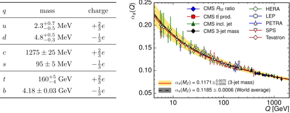
Table 2.1: The table shows the electric charge (in units of the positive elementary charge e) and the quark masses obtained from fits to experimental data taken from ref. [48]. The light quark masses of u, dand s quarks are given at the MS scale µ = 2 GeV. The masses of the heavy quarks are given at the MS scale which equals their own mass. Note that these masses are strongly scheme and scale dependent. E.g., the top mass obtained from a pole-mass definition yields a value that lies roughly 13 GeV higher.

q mass charge

u 2.3^+0.7_−0.5MeV +²₃e d 4.8^+0.5_−0.3MeV −¹3e c 1275±25 MeV +²₃e

s 95±5 MeV −¹3e

t 160⁺⁵₋₄GeV +²₃e b 4.18±0.03 GeV −¹3e

10 100 1000

Q[GeV]

0.05 0.10 0.15 0.20 0.25 αs(Q)

αs(MZ) = 0.1171±^0.0075_0.0050(3-jet mass) αs(MZ) = 0.1185±0.0006 (World average)

CMSR32ratio CMS tt prod.

CMS incl. jet CMS 3-jet mass

HERA LEP PETRA SPS Tevatron

Figure 2.1: The picture shows the running of the strong couplingα_s= ^g_4π² in the perturbative regime. Here Qcorresponds to the MS scale. This figure has been taken from ref. [49].

Pure QCD has seven free parameters that have to be specified and are determined from experiment: the 6 quark masses and the coupling constant given in table 2.1 and figure 2.1, respectively. One immediately notices the strong hierarchy in the quark masses

mu.mdms<ΛQCDΛhad.< mc < mbmt, (2.6) where Λ_QCD ≈ 200 MeV is the typical scale of nonperturbative effects in QCD (to be more specific: it corresponds to the scale where the perturbatively calculated running of the coupling shown in figure 2.1 would diverge) and Λhad.≈1 GeV is the scale of the lowest-lying nonpseu- doscalar hadrons. Sincem_u, m_d andm_s have values below the relevant scales of QCD, we may consider them as approximately massless (i.e., we start without masses and introduce them as a small perturbation later on). A reexamination of the fermionic term in the QCD Lagrangian density,

X

a

¯

q^a i /D−ma)q^a=X

a

¯

qâ_Li /Dq_Lâ + ¯q_Râi /Dqâ_R−mâq¯â_Rq_Lâ−mâq¯_Lâq_Râ

, (2.7)

shows that quarks of different chiralities, q_L/R=γ_L/Rq= ¹₂(1∓γ5)q, are coupled by the mass term only. This enables us to perform symmetry transformations individually on left- and right- handed quarks, such that the QCD Lagrangian is approximately symmetric under global

SU(nf)L⊗SU(nf)R⊗U(1)L⊗U(1)R, (2.8)

(19)

2.1. LOW-ENERGY EFFECTIVE THEORY FOR QCD transformations, where n_f is the number of light quarks equal to three or two, depending on whether one treats the strange quark as light or not.⁴ On a classical level, these symmetries correspond to the conservation of the currents

j_L/R,µⁱ = ¯qγµγ_L/Rσⁱq , j_L/R,µ= ¯qγµγ_L/R1q , q= q^u q^d

!

, fornf = 2 , (2.9a)

j_L/R,µⁱ = ¯qγµγ_L/Rλⁱq , j_L/R,µ= ¯qγµγ_L/R1q , q=



 q^u q^d q^s



 , fornf = 3 , (2.9b)

by virtue of the Noether theorem [51]. σⁱ andλⁱ are Pauli and Gell-Mann matrices acting on flavor space, and the superscript ican take values between 1 andn²_f−1. These currents can be combined to the usual vector and axialvector currents:

V_µⁱ=j_R,µⁱ +j_L,µⁱ , Aⁱ_µ=j_R,µⁱ −j_L,µⁱ , (2.10a) Vµ=jR,µ+jL,µ , Aµ=jR,µ−jL,µ. (2.10b) It is already clear that, apart from the U(1)V case, these currents can only be partially conserved:

in the presence of degenerate light quark masses the Lagrangian (2.7) is only invariant under vectorial symmetry transformations. If the masses of the light quarks differ from each other also the SU(nf)V symmetry is broken explicitly. However, the predominant reason for the breaking of the axial symmetries lies elsewhere. U(1)_Ais broken due to the axial anomaly [52], which gives rise to the coupling ofη⁰(the physical statesηandη⁰are mixtures ofη⁰andη⁸) to two gluons and yields a nonvanishing mass ofη⁰in the chiral limit (i.e., the limit of vanishing quark masses). In pure QCD without other standard model interactions the currentsAⁱ_µdo not exhibit an anomaly.

But, as is well known, the continuity equations for Aµ,A³_µ and A⁸_µ are broken anomalously due to QED effects which opens the electromagnetic decay channelsπ⁰, η, η⁰ →γγ. Historically, the π⁰ → γγ decay was the first measurement of the axial anomaly. It has a branching fraction of >98% leading to a rapid decay of the π⁰ (compare the mean lifetime τ(π⁰) = 8.4×10⁻¹⁷s versus the mean lifetime of the charged pions τ(π^±) = 2.6×10⁻⁸s due to weak decays; cf.

ref. [48]).

Neglecting the explicit breaking of the symmetries for a moment, we find conserved charges for the symmetries which are not broken anomalously in QCD:∂µj^µ= 0, wherej can beVⁱ,Aⁱ and V from eq. (2.10). Using a simple quantum mechanical argument (see, e.g., ref. [53]) one can show that this leads to the occurrence of hadron multiplets with degenerate mass: being conserved, the currents commute with the QCD Hamiltonian, [HQCD, Q] = 0, such that one finds for any hadronic state |hiat zero three-momentum and with mass m_h

4Yet another symmetry of a massless QCD Lagrangian is conformal symmetry. It is broken by quantum effects and we will not discuss it in detail here. See, e.g., ref. [50] for a review.

(20)

degeneracy is realized almost exactly for the isospin multiplets in the hadron spectrum. Re- calling the mass differences within the baryon octet (up to mΞ−mN ≈377 MeV; cf. [48]) one immediately sees that this is not the case for n_f = 3. This can be attributed to the rather large explicit symmetry breaking due to the strange quark mass. For the axialvector currentsh⁰ has inverse parity compared to h, which means that each hadron should have a parity partner of similar mass. This is not the case at all. Even for n_f = 2 the mass difference between a nucleon and its (lowest-lying) parity partner ismN^∗−mN ≈597 MeV (cf. [48]). The way out of this dilemma is the interpretation of|h⁰ias a threshold state|hπiwith a massless pseudoscalar hadronπ. The necessary massless bosons are provided by a well-known mechanism: according to the Nambu–Goldstone theorem [54, 55],N massless bosons (so-called Goldstone bosons (GBs)) occur when a global symmetry created from N generators (in our case N =n²_f −1) is broken spontaneously, which means that the Lagrangian is invariant under symmetry transformations, while the ground state is not (a detailed description is given in section 2.1.2). In QCD the symmetry is, in addition, broken explicitly due to nonzero quark masses which provides also the GBs with a mass, and allows us to identify them with the three pions (in case ofn_f = 2) or the pseudoscalar meson octet (if nf = 3) in the experimentally measured hadron spectrum.

We can summarize that symmetries in QCD are broken in manifold ways: U(1)A is broken anomalously and explicitly, SU(n_f)_L⊗SU(n_f)_Ris broken spontaneously to SU(n_f)_V,⁵which in turn is broken explicitly. The only global symmetry of those stated above that stays completely intact is U(1)_V, which guarantees exact baryon number conservation.

2.1.2 Spontaneous breaking of the chiral symmetry

Spontaneous symmetry breaking (SSB) is by no means a phenomenon limited to quantum field theories. It can be encountered in nearly every branch of physics. A simple example from classical mechanics is a particle of mass m sliding (without friction) along a ring (with radiusR) that rotates around its vertical axis in a gravitational field with angular velocityω (cf. refs. [57, 58]

and figure 2.2(a)). After implementing the constraints the Lagrangian function of such a system reads

L=1

2mR² θ˙²+ω²sin²(θ)

+mgRcos(θ), (2.12)

where the symmetry under the parity transformation of the angle θ→ −θis evident. Using the Euler–Lagrange equations of motion one finds static solutions if

0 = sin(θ)

cos(θ)− g Rω²

. (2.13)

For ω² < _R^g there is only one stable equilibrium position atθ= 0. However, for larger angular velocities (ω² > _R^g) the solution at θ = 0 becomes unstable and two ground-state solutions at θ = ±arccos _Rω^g2

occur. In contrast to the Lagrangian, the latter ground states are not symmetric under the parity transformation mentioned above, which means that the symmetry is broken spontaneously.

5In ref. [56] it is shown, that a spontaneous breaking of the vectorlike global symmetries is not possible in QCD.

(21)

2.1. LOW-ENERGY EFFECTIVE THEORY FOR QCD

θ ω

g

R m

(a)

ϕ₁ ϕ₂

V

(b)

Figure 2.2: Subfigure (a) shows the setup for a massive particle that slides frictionlessly along a hoop rotating around its vertical axis in a gravitational field. This is a simple example from mechanics of a system that exhibits SSB of a discrete symmetry. Subfigure (b) is a plot of the so-called Mexican hat potentialV used in eq. (2.14), which is the prime example for a potential that leads to SSB.

The situation described in the last paragraph is an example for the breaking of a discrete symmetry. In the continuous case one has to differentiate between global symmetries and local gauge symmetries. As already mentioned in the last section in the context of chiral symmetry breaking, the spontaneous breaking of a global symmetry leads to the occurrence of a massless boson for each broken generator. Another typical example for SSB of a global symmetry are ferromagnets (below the Curie temperature), where the alignment of the spins in the ground state breaks rotational invariance.⁶ As pointed out by Higgs [60, 61], the spontaneous breaking of a gauge symmetry does not necessarily lead to massless bosons. Instead, the affected gauge bosons acquire a mass and a longitudinal degree of freedom.

Let us illustrate the spontaneous breaking of a continuous global symmetry using a complex boson field (this example dates back to Goldstone himself [54]). Consider the Lagrangian density

L=1

2(∂µϕ^∗)∂^µϕ−V(ϕ^∗ϕ) =1

2(∂µϕ^∗)∂^µϕ+µ²₀

2 ϕ^∗ϕ−λ0

4 (ϕ^∗ϕ)², (2.14) where ϕ =ϕ₁+iϕ₂, with real-valued fields ϕ₁ and ϕ₂. Obviously, L is invariant under phase transformationsϕ→e^iαϕ. The parameterλ0 has to be positive in order to have a lower bound for the potential. Ifµ²₀<0 the potential has a unique minimum at|ϕ|= 0. Forµ²₀>0, however, the potential has a minimum at χ, where |χ|=µ0/√

λ, while the phase is undetermined, which yields an infinite set of possible vacua as illustrated in figure 2.2(b). The choice of a specific phase for the vacuum destroys (or hides) the symmetry. We can expand the Lagrangian (2.14) around the vacuum using the new variable ϕ⁰ =ϕ−χ. For real and positiveχthe result reads

L=1

2 (∂µϕ⁰₁)∂^µϕ⁰₁−2µ²₀ϕ⁰²₁ +1

2(∂µϕ⁰₂)∂^µϕ⁰₂−λ0χϕ⁰₁ϕ^0∗ϕ⁰−λ0

4 (ϕ^0∗ϕ⁰)²−χ⁴

, (2.15)

6Actually, in the ferromagnet only one Goldstone boson occurs, instead of the two one would expect naively.

Such a reduction of GBs in the spectrum can happen in Lorentz-noninvariant systems, if two Goldstone boson modes occur as canonically conjugate pair that corresponds to one joint degree of freedom (see ref. [59]).

(22)

where the absence of the mass term forϕ⁰₂ identifies it as the Goldstone boson.

Finding the correct low-energy description of QCD is a much less trivial task: since the SSB occurs dynamically on the level of the hadrons, it is an entirely nonperturbative effect, which means that (in contrast to the example above) we do not have direct access to the potential that governs the symmetry breakdown. However, already the knowledge of the underlying group theoretical structure, i.e., SU(n_f)_R⊗SU(n_f)_L →SU(n_f)_V in case of QCD, enables us to derive the transformation properties of the Goldstone bosons by group theoretical means. Our description of this procedure follows the derivations given in refs. [62–64] (cf. also [35]). For fundamental group theory definitions the reader may consult ref. [65].

Let Φ∈P be a field containing the Goldstone bosons, whereP is the set of all possible field configurations. We omit the dependence on the spacetime position, since it is not relevant for our discussion (see ref. [64] for details). The operation of the group G on P is given by the mapping

f : G×P →P , (g,Φ)7→Φ⁰ , (2.16)

where the identity1∈Ghas to map each field configuration onto itself, and consecutive action of group elements has to fulfill the group homomorphism property (2.17b). Additionally, we require that all field configurations are connected by symmetry transformations. Hence, we have

f(1,Φ) = Φ, (2.17a)

f(g1, f(g2,Φ)) =f(g1◦g2,Φ), (2.17b)

∀Φ,Φ⁰∈P , ∃g∈G : f(g,Φ) = Φ⁰ . (2.17c) The goal of this paragraph is the determination off. Using the properties of the mappingf one can check explicitly that the set H of group elements under whose action the ground state (i.e., the orgin ofP at Φ = 0) remains unaffected,

H =

g∈Gf(g,0) = 0 , (2.18)

forms a subgroup ofG, which is sometimes called the stability group of the origin [66]. Looking at the definition ofH, it is clear that it corresponds to the (largest possible) subgroup ofGwhich is not broken spontaneously. Next, we define

GH =

gH g∈G , (2.19)

which is the set of all left cosetsgH={g◦h|h∈H}. For all elements of a left cosetf maps the origin onto the same field configuration, which can be easily verified using eq. (2.17b). Hence,f induces a mapping ˜f of the set of left cosets onto the space of Goldstone boson fields:

f˜ : G

H →P , f˜(gH)7→f(g,0) . (2.20) This mapping is isomorphic: its surjectivity follows directly from eq. (2.17c), while its injectivity can be proven by showing that for allg, g⁰ ∈Git holdsf(g,0) =f(g⁰,0)⇒g⁰ ∈gH:

0 =f(1,0) =f(g⁻¹◦g,0) =f(g⁻¹, f(g,0)) =f(g⁻¹, f(g⁰,0)) =f(g⁻¹◦g⁰,0),

⇒g⁻¹◦g⁰ ∈H ⇒g⁰ ∈gH .

(2.21)

(23)

2.1. LOW-ENERGY EFFECTIVE THEORY FOR QCD Therefore, each field configuration Φ =f(r_Φ,0) corresponds to a left cosetr_ΦH, where one may choose a convenient representative rΦ for each left coset. The inherent beauty of this relation is that it allows us to determine the operation of the symmetry group on the Goldstone boson fields (described by f) from the action of the corresponding group elementsg on the left coset rΦH, which is simplyg◦rΦH. The situation can be visualized by the commutative diagram [64]

r_ΦH r⁰_ΦH =g◦rΦH .

Φ Φ⁰

f

f˜ ∼ g

f˜ ∼ (2.22)

Thus, the transformation properties of the Goldstone bosons are uniquely determined by the geometry up to reparametrizations of G

H.

After the discussion of the underlying group theory, we may now move on to its practical application in (massless) QCD, where the chiral symmetry group is broken spontaneously to its vectorial subgroup:

G= SU(n_f)_L⊗SU(n_f)_R=

(L, R)L, R ∈SU(n_f) , (2.23a) H= SU(n_f)_V =

(V, V)V ∈SU(n_f) . (2.23b)

We can now choose a representative r_Φ forg_ΦH, withg_Φ= (L_Φ, R_Φ)∈G, that is characterized by a unique matrix UΦ∈SU(nf) [64]:

g_ΦH= (L_Φ, R_Φ)H= (L_Φ, R_ΦL^†_ΦL_Φ)H = (1, R_ΦL^†_Φ)◦(L_Φ, L_Φ)H

= (1, R_ΦL^†_Φ)H≡(1, U_Φ)H ,

(2.24) i.e., we choose the representative always in such a way that the first component is the identity.

This choice is particularly convenient, since it leads to a simple transformation behavior of the representative matrix:⁷

Φ⁰∼=r_Φ⁰H = (1, U_Φ⁰)H

=! g◦r_ΦH= (L, R)◦(1, U_Φ)H = (L, RU_ΦL^†L)H= (1, RU_ΦL^†)H ,

⇒U_Φ⁰ =RU_ΦL^† .

(2.25)

Hence, we can represent the Goldstone pseudoscalars by a SU(nf) matrixU (we will drop the index from now on) with simple transformation properties and the remaining freedom amounts to the choice of a parametrization for SU(nf) matrices. A widespread and (for most purposes) convenient choice are canonical coordinates

U =eⁱ^F^Φ⁰ , with





Φ =P3

i=1φⁱσⁱ , fornf = 2, Φ =P⁸

i=1φⁱλⁱ , fornf = 3,

(2.26)

7Fixing the second component to be the identity and using the first one as the representative would be similarly convenient, and would lead to the transformationU_Φ0=LUΦR^†, which is also found in the literature.

(24)

where σⁱ and λⁱ correspond to Pauli and Gell-Mann matrices, respectively, and F₀ is the pion decay constant in the chiral limit [67]. Theφⁱare real-valued such that Φ is Hermitian (Φ^†= Φ).

The components of Φ can be identified with the pseudoscalar mesons:⁸ Φ =√

2

√1

2π⁰ π⁺ π⁻ −^√¹₂π⁰

!

, fornf = 2, (2.27a)

Φ =√ 2







√1

2π⁰+^√¹

6η π⁺ K⁺

π⁻ −^√¹₂π⁰+^√¹

6η K⁰

K⁻ K⁰ −^√²₆η





 , fornf= 3 , (2.27b)

which corresponds to the convention where F_π = F₀+O(m²_π, m²_K, m²_η)≈ 92 MeV. After the choice of a parametrization, eq. (2.25) fixes the transformation properties of the Goldstone bosons. For all parametrizations that map the origin (Φ = 0) onto the identity one finds that the pseudoscalar fields transform particularly simple under chiral rotations along the unbroken vectorial subgroup: Φ⁰ = VΦV^†. For general chiral rotations the transformation law is nonlinear (one therefore speaks of a nonlinear realization of chiral symmetry, cf. refs. [66, 68]) and depends on the explicit choice of parametrization. Note that the seeming ambiguity due to the free choice of a parametrization is not a problem, since all possible realizations of the symmetry are equivalent [68].

2.1.3 Meson chiral perturbation theory

In the last section we have derived the general form of the Goldstone boson fields occurring in an effective theory of QCD. They can be represented by a unique SU(nf) matrix U, which has a definite transformation behavior under chiral rotations (see eq. (2.25)). At low energies E Λ_had. the heavier particles in the hadron spectrum decouple from the theory, i.e., they can be integrated out, see, e.g., ref. [69]. Hence, an effective Lagrangian for massless QCD can only consist of combinations of the field U and derivatives, that are invariant under both Lorentz transformations and chiral rotations. Unfortunately, there are infinitely many possible contributions and an arbitrary choice of terms would automatically lead to a model dependence.

The solution to this problem is chiral perturbation theory, which is based on the observation that every occurrence of a derivative in a vertex leads to a suppression by a factorp∝E/Λhad.. Therefore, we can arrange the terms in the effective Lagrangian according to their order in p denoted by the superscript in parentheses:

L^M =L⁽²⁾M +L⁽⁴⁾M +L⁽⁶⁾M +. . . . (2.28) The series contains only even powers of pdue to Lorentz invariance, and starts at 2, since the only zeroth order term tr

U^†U =nf is an irrelevant constant. However, this approach would be pointless if one would have to evaluate an infinite number of Feynman loop diagrams in order to obtain a result to a desired accuracy, say p^D. That this is not the case is guaranteed by the

8One should note that this identification fixes the phase conventions.

(25)

2.1. LOW-ENERGY EFFECTIVE THEORY FOR QCD Weinberg power counting theorem [38], which provides the order D of a Feynman diagram in terms of the number of loopsNL and the number of verticesN_M⁽ⁿ⁾from L⁽ⁿ⁾M :

D= (d−2)NL+ 2 +X

n

(n−2)N_M⁽ⁿ⁾, (2.29)

where we are usually interested in the case with spacetime dimensiond= 4. Using dimensional regularization the respective diagram is suppressed by a factor p^D. Thus, for any given order p^D the number of loops in the contributing Feynman diagrams is limited toNL ≤ ^D2 −1. The lowest order part of the effective Lagrangian is rather simple. In the massless case it consists of one term only:

L⁽²⁾M

_m

q=0

=F₀² 4 tr

(∂_µU^†)∂^µU , (2.30)

where the coefficient is (by convention) chosen in such a way that (after expanding the exponential U) the prefactor of the kinetic term for the mesons is independent of the decay constant. As argued in ref. [70], 4πF₀ ' 1 GeV plays the role of the chiral symmetry breaking scale Λ_had.. One can show that all other possible contributions of lowest order are either equivalent or vanish by using the identities

0 = (∂_µU)U^†+U(∂_µU^†) = (∂_µU^†)U+U^†(∂_µU), (2.31a) 0 = tr

(∂_µU)U^† = tr

(∂_µU^†)U . (2.31b)

As expected,L⁽²⁾M

_m

q=0 does not contain a mass term for the pseudoscalar fields.

So far we have only considered the chiral limit, where the quarks are massless. However, in the real world, chiral symmetry is broken explicitly due to finite quark masses. In order to implement the explicit breaking systematically into the low-energy theory, we apply the source field formalism developed in refs. [67, 71]: in this formalism one implements the coupling of massless QCD to external (color-singlet) vector, axialvector, scalar and pseudoscalar background fields by adding the appropriate source term

L^S[vµ, aµ, s, p] = ¯q(γ^µvµ+γ^µγ5aµ)q−q(s¯ −iγ5p)q

= ¯qRγ^µ(vµ+aµ)qR+ ¯qLγ^µ(vµ−aµ)qL−q¯R(s+ip)qL−q¯L(s−ip)qR .

(2.32) to the Lagrangian of massless QCD. The external fields are Hermitian matrices in flavor space.

Disregarding the anomalous breaking described in section 2.1.1, which would yield corrections starting from O(p⁴) [71], the full theory is invariant underlocal chiral rotations

qR(x)→R(x)qR(x), qL(x)→L(x)qL(x), whereR(x), L(x) ∈U(nf), (2.33) if the external fields transform as follows:

(v_µ+a_µ)→R(v_µ+a_µ)R^†+iR∂_µR^† , (2.34a) (v_µ−a_µ)→L(v_µ−a_µ)L^†+iL∂_µL^† , (2.34b)

(s+ip)→R(s+ip)L^† . (2.34c)

(26)

The last term in the transformation law for the right- and left-handed vector fields (r_µ =v_µ+a_µ andlµ=vµ−aµ) allows us to interpret the vectorial part of the source term as the second half of a covariant derivative, and is therefore responsible for the upgrade of the global symmetry (in pure QCD) to a local gauge symmetry (in the full theory). Obviously, one can restore massless QCD by setting all external fields to zero. However, the beauty of the formalism lies in the fact that one can evaluate nontrivial background field configurations. In particular, we obtain the case we are interested in (massive QCD), by settingvµ,aµ andpto zero, and the scalar field to its nonvanishing vacuum expectation values=M, whereMis the diagonal quark mass matrix.

Actually, M is diagonal, because we define the quark fields to be the mass eigenstates of the theory.

To introduce the explicit chiral symmetry breaking also in the low-energy theory, we simply have to add all possible scalar source terms to the theory. By setting them to the correct vacuum expectation value the quark masses are taken into account systematically. The two possible structures of lowest order including scalar and pseudoscalar source terms are

tr

(s+ip)U^†±(s+ip)^†U . (2.35)

They have positive/negative parity (under parity transformation s→s, p→ −pand U ↔U^† together with an inversion of the position in space; see also section 2.2) and, therefore, only the

“+” combination is relevant for the leading Lagrangian density. In the limit s=M andp= 0 the latter reads

L⁽²⁾M =F₀² 4 tr

∂_µU^†∂^µU +F₀²B₀ 2 tr

M U+U^† , (2.36)

whereB₀is the so-called condensate parameter in the chiral limit. The additional term provides the pseudoscalar Goldstone bosons with a mass, thereby promoting them to pseudo Goldstone bosons. Since the mass enters the propagator at the same level as the momentum, it turns out to be convenient to count the quark mass matrix (or rather scalar and pseudoscalar external fields) as orderp²in the ChPT bookkeeping, which explains why we have added the lowest order source term to L⁽²⁾M. With this choice also the hierarchical order in the EFT Lagrangian (2.28) and the power counting formula (2.29) hold unchanged. The higher order Lagrangians of the meson sector are not relevant for the projects presented in this work. We refer the reader to refs. [67, 71] for more details. A review of state of the art calculations in the mesonic sector at two-loop order (i.e., O(p⁶)) can be found in ref. [72].

To conclude this section, let us emphasize that the effective field theory we have constructed is Lorentz-covariant. Hence, the requirement for low energies of the external particles only has to be fulfilled in one freely choosable frame, and one can boost the result to any frame of interest, which means that ChPT is actually applicable to a much larger set of problems than one might think at first sight.

2.1.4 Baryon chiral perturbation theory

So far we have only considered a low-energy theory of QCD that was limited to the dynamics of the pseudo Goldstone bosons. This section is dedicated to the inclusion of J^P = ¹₂⁺ ground-

(27)

2.1. LOW-ENERGY EFFECTIVE THEORY FOR QCD state baryons. We restrict ourselves to the cases where one baryon occurs in the initial and one in the final state. The main obstacle connected to the description of baryons within the low-energy theory is their nonzero mass in the chiral limit, which introduces an additional large scalem0∼Λhad. into the theory. Therefore, only the baryon three-momentum can be required to be small (of order p¹ in the ChPT counting scheme), while its energy is large (order p⁰). In particular in loop diagrams containing both baryonic and mesonic propagators, the additional scale leads to problems with the usual power counting, whose solution will be addressed in section 2.1.5. One usually works in a quenched approximation, i.e., closed baryonic loops are neglected,⁹anticipating that they can be integrated out, and that their effect is parametrized by low-energy constants (LECs) without loss of generality.

The baryons are built from three valence quarks and should, therefore, be classified into flavor multiplets that transform under the following irreducible representations of the vectorial subgroup

2⊗2⊗2 = 2⊕2⊕4 , fornf = 2 , (2.37a) 3⊗3⊗3 = 1⊕8⊕8⊕10, fornf = 3 . (2.37b) Since the vectorial subgroup is only broken explicitly due to quark mass differences, the baryons within one multiplet are mass-degenerate, as long as the masses of the light quarks are equal.

The totally antisymmetric flavor structure (corresponding to 1) cannot occur in ground-state baryons (i.e., baryons with a symmetric spatial wave function), since this would require a totally antisymmetric spin wave function. The latter is simply impossible for the same reason for which no singlet flavor structure occurs in the two-flavor case: one cannot form a structure that is totally antisymmetric in three indices, if one has only two possible values for the indices to choose from. The four- and ten-dimensional representations lead to totally symmetric flavor multiplets corresponding to the Delta baryons and the full baryon decuplet, respectively, which have spin ³₂. Of the two remaining two-dimensional (eight-dimensional) multiplets one has a mixed-symmetric and one a mixed-antisymmetric flavor structure, i.e., they are symmetric/antisymmetric under exchange of the flavors of the first and the second quark. However, under exchange of the third quark with one of the others, the two multiplets do mix with each other, such that only one doublet (octet) occurs in the hadron spectrum. In ChPT, the spin ¹₂ baryons are usually represented by the nucleon doublet (in case of nf = 2) or by a traceless 3×3 matrix which contains the octet (in case ofnf = 3) [74]:

n_f = 2 : Ψ = p n

!

, (2.38a)

nf = 3 : B=







√1

2Σ⁰+^√¹

6Λ Σ⁺ p

Σ⁻ −^√¹₂Σ⁰+^√¹

6Λ n

Ξ⁻ Ξ⁰ −^√²₆Λ





≡κpp+κnn+. . . , (2.38b)

9Note, that this does not at all mean that the resulting theory is a description of quenched QCD (for such a variety of ChPT see, e.g., ref. [73]). We simply refer to the methodical similarity of neglecting closed fermionic loops.

(28)

p n

Σ⁺ Σ⁰

Σ⁻

Ξ⁰ Ξ⁻

Tˆ₋

−Uˆ₋

−Vˆ₋

−Tˆ₋/√ ˆ 2

T₋/√ 2

Vˆ₋ Uˆ₋

−Tˆ₋

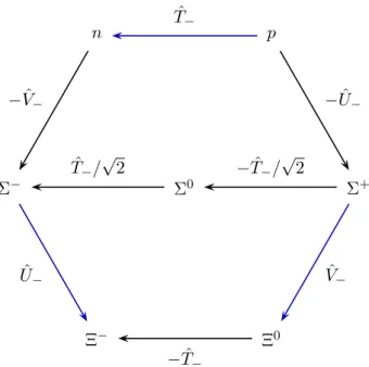
Figure 2.3: Illustration of our phase conventions. The Λ baryon is not shown since one needs a linear combination for the construction of its wave function, cf. eq. (2.41c). The blue arrows will be relevant in chapter 4. They indicate the cases where one has to apply a Fierz transformation (see ref. [76]) to relate the distribution amplitudes at the symmetric point. An explicit calculation shows that this always yields an additional minus sign that has to be taken into account in order to reproduce eq. (4.73) and eq. (4.74). This figure is taken from our work [75] and was created by M. Gruber.

where the second line defines the matrices κB. The choice of phases (or rather the absence of them) in these definitions fixes our phase conventions to a large extent (cf. also our article [75]).

To see this, consider the isospin ( ˆT₋), u-spin ( ˆU₋) and v-spin ( ˆV₋) lowering operators, which are defined via their action on specific quark flavors: ˆT₋u =d, ˆU₋d = s, ˆV₋u = s and zero otherwise. If one identifies the flavorsu,dandswith the first, second and third unit vector in a three-dimensional space, respectively, the matrix representations of the lowering operators read

T₋=





0 0 0 1 0 0 0 0 0



 , U₋=





0 0 0 0 0 0 0 1 0



 , V₋=





0 0 0 0 0 0 1 0 0



 . (2.39)

We now identify each baryon B with the associated 3×3 matrix κB and we further define the action of the lowering operators ˆT−, ˆU− and ˆV− on the octet by the usual expressions for the adjoint representation without any additional phase factors:

Tˆ₋κ_B = [T₋, κ_B], Uˆ₋κ_B = [U₋, κ_B], Vˆ₋κ_B= [V₋, κ_B]. (2.40) The above choices specify our phase conventions. Starting from the proton state, the complete