Ludwig-Maximilians-Universität München
Faculty of Physics Physics Master
Master Thesis
Dark Matter Production in Warped Extra-Dimensions
Arturo de Giorgi
Munich, November 26, 2020
Ludwig-Maximilians-Universität München
Fakultät für Physik Physik Master
Masterarbeit
Dunkle-Materie-Produktion in verzerrten Extradimensionen
Arturo de Giorgi
München, November 26, 2020
Master thesis carried out at the Max Planck Institute for Physics under the supervision of:
PD Dr. habil. Georg Raffelt Dr. Stefan Vogl
Munich, November 26, 2020
Abstract
In this thesis, an extra-dimensional model for Dark Matter is studied. The Dark Matter is assumed to be a massive scalar particle interacting only gravitationally in the extra-dimensional Randall-Sundrum scenario. The annihilation of Dark Matter into Kaluza-Klein (KK) modes, Radions and Standard Model particles is analyzed. Denoting with s the centre of mass energy squared of the process, the amplitudes for to the production of KK-modes are found to be of O (s
3) . Such a growth would imply a breakdown of the theory at scales much lower than its fundamental scale. This type of issue is well- known in massive gravity and there is no general solution to it. It is here proved analytically that in the Randall-Sundrum scenario, this anomalous growth in energy is reduced to O (s) once the contributions of all KK-modes and of the Radion are taken into account and summed properly. Studying the relic abundance of Dark Matter in the context of the freeze-out mechanism, we find that the allowed parameter space of the theory is much smaller than what had been found previously in the literature.
Lastly, the bounds, derived from the data of diphoton production from LHC Run II, are considered.
Contents
Introduction 1
1 Dark Matter in a Homogeneous Universe 3
1.1 Dark Matter . . . . 3
1.2 Ideal Fluid in a Homogeneous Universe . . . . 5
1.3 Equilibrium Thermodynamics in a Homogeneous Universe . . . . 7
1.4 The Boltzmann Equation . . . . 9
1.4.1 The Boltzmann Equation . . . . 9
1.4.2 The Integrated Boltzmann Equation in Flat FLRW Universe . . . . 10
1.4.3 The Yield . . . . 12
1.5 The Freeze-Out Mechanism . . . . 13
1.5.1 Freeze-Out of Non-Relativistic Species . . . . 14
2 The Randall-Sundrum Model 16 2.1 The Model . . . . 16
2.1.1 The Action and the Randall-Sundrum Metric . . . . 16
2.1.2 Solution to the Hierarchy Problem . . . . 19
2.2 Weak Field Expansion . . . . 20
2.2.1 Gauge Redundancy and Physical Degrees of Freedom . . . . 20
2.2.2 Einstein Frame Parametrization and Lagrangian Expansion . . . . 23
2.3 4D Particle Content . . . . 23
2.3.1 The Mass Equation & KK-Gravitons . . . . 24
2.3.2 The Radion . . . . 26
2.4 Couplings of the Theory . . . . 27
2.4.1 Couplings on the IR brane: Coupling of Gravity to Matter . . . . 28
2.4.2 Couplings in the Bulk: Gravity’s Self Couplings . . . . 29
3 Dark Matter Annihilation 32 3.1 Dark Matter in this Thesis . . . . 32
3.2 The Helicity Method . . . . 32
3.2.1 The Method . . . . 33
3.3 Amplitudes of the Annihilations . . . . 34
3.3.1 Annihilation into SM particles . . . . 34
CONTENTS
3.3.2 Annihilation into Radions: φφ −→ rr . . . . 37
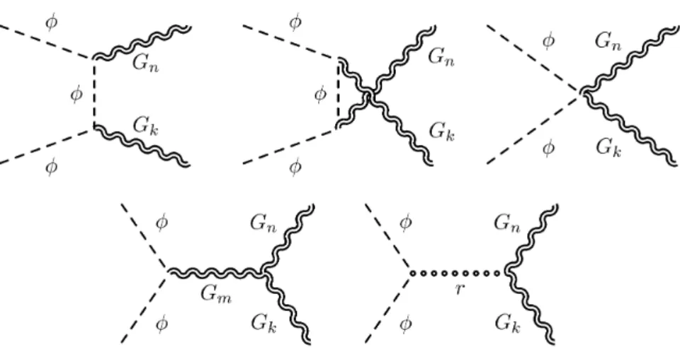
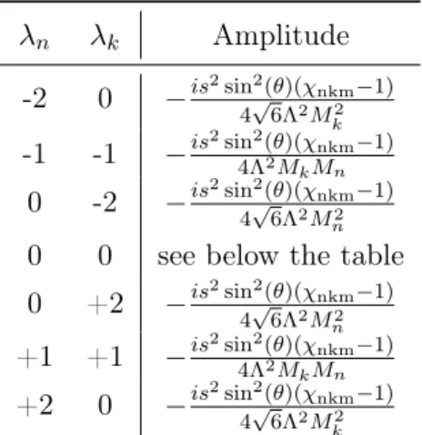
3.3.3 Annihilation into Gravitons: φφ −→ G
nG
k. . . . 38
3.3.4 Annihilation into Radion & Graviton: φφ −→ rG
n. . . . 40
3.4 Sum Rules for the Couplings . . . . 41
3.4.1 Main Parameters and Basic Properties . . . . 42
3.4.2 Derivation of the Sum Rules . . . . 43
3.4.3 Numerical Analysis . . . . 49
3.5 Unitarity Constraint . . . . 51
4 Dark Matter Phenomenology in the Randall-Sundrum Model 53 4.1 Bounds on the Randall-Sundrum Model from LHC Run II . . . . 53
4.1.1 Proton-Proton Collision . . . . 53
4.1.2 Bounds from Diphotons Production: P P −→ G
1−→ γγ . . . . 55
4.2 Freeze-Out in the Randall-Sundrum Model . . . . 57
4.2.1 m
φ∈ [0.3, 8] TeV - M
1∈ [0.5, 10] TeV . . . . 59
5 Conclusions 62 Appendices 65 A Mathematica Packages Used 67 B Expansion of the RS-Lagrangian and Vacuum Energy Cancellations 68 B.1 Overview and Expansion of the Volume Element . . . . 68
B.2 0th Order . . . . 71
B.3 1st Order . . . . 71
B.4 2nd Order . . . . 72
B.5 3rd Order . . . . 74
C Feynman Rules 76 C.1 Vertices . . . . 76
C.1.1 Vertices involving only RS particles . . . . 77
C.1.2 Vertices involving RS & SM particles . . . . 78
D Annihilation Cross Sections of Dark Matter into SM particles 82 D.1 Annihilation through Graviton(s) . . . . 82
D.2 Annihilation through Radion . . . . 83
E Decay Widths of Graviton(s) and Radion 84 E.1 Graviton(s) Decay Widths . . . . 84
E.1.1 Graviton(s) - Decay Width into SM particles . . . . 84
E.1.2 Graviton(s) - Decay Widths into RS particles . . . . 85
E.1.3 Approximation of Γ
n. . . . 85
E.2 Radion Decay Widths . . . . 86
CONTENTS
E.2.1 Radion - Decay Widths into SM particles . . . . 86 E.2.2 Radion - Decay Widths into RS particles . . . . 87
Glossary 88
Bibliography 90
Acknowledgements 94
Introduction
The nature of Dark Matter (DM) remains one of the biggest open questions in physics. Since hydrodynamically it seems to behave as dust, the simplest assumption is to consider DM as made of some type of unknown particle. Its reluctance to interact with Standard Model particles becomes the key element to a world of models: sterile neutrinos, WIMPs and Axions are some of the most studied possibilities [1]. Since we know of its existence only through its gravitational force, an interesting possibility is that this particle only interacts gravitationally. Another fascinating possibility is the existence of extra dimensions invisible to us. If this was the case, General Relativity (GR) would have to be recovered in the 4D-Effective Field Theory (EFT) [2, 3, 4]. In this context, particularly notable is the Randall-Sundrum (RS) model [5], which through a compact warped 5th-dimension solves elegantly the hierarchy problem between the Planck and the Higgs scales and naturally includes gravitational interactions much stronger compared to GR. Such a stronger coupling makes the theory, from a phenomenological point of view, more appealing than GR, since it leads to predictions that could be tested in the near future at colliders. These features make this model and its combination with Dark Matter a very intriguing pair to be studied.
In this thesis, we study in detail the production of Dark Matter in the early universe via freeze- out mechanism. The Dark Matter is assumed to be a massive scalar particle which interacts only gravitationally in the Randall-Sundrum scenario. In our model, the SM particle content lives on a boundary of the 5th dimension usually called TeV-brane . We study in detail the particle content of the RS model, with particular attention to the role of the Kaluza-Klein (KK) modes of the 4D-EFT. DM models in the RS scenario have been studied in the literature [6, 7], but here not only the annihilation of DM into SM, but also into RS particles, is investigated in detail. A subtle problem arises in this context. The scattering amplitude of massive spin-2 fields exhibits a huge growth in the high energy limit and poses a strong problem to unitarity, resulting in a break down of the theory at energies much below the fundamental scale [8]. This issue is well known in massive gravity and general methods of constructing theories avoiding this problem are still being studied [9, 10, 11]. However, since the the original 5D theory only contains one fundamental scale as dimensionful parameter, it is expected to be well behaved up to that scale. This suggests that the resulting 4D-EFT can be healed if the contribution from all the 4D-EFT-particles are considered. Of course, the contribution of a single KK-mode does not reflect the whole 5D theory and is therefore affected by the unitarity issue. The problem is solved only when the full RS-particle content is included in the computation. Even though the details of this mechanism have not been analyzed in general, it has been recently shown [12, 13, 14]
that this is indeed the case for the for the scattering of KK-modes in warped-extra dimensions, where
the energy growth can be reduced from O (s
5) to O (s) . In this thesis, building on the same approach,
CONTENTS
we prove analytically that this is also the case for the annihilation of DM in RS particles, and derive new subtle relations between the couplings of KK-modes that ensure the cancellation of high energy terms.
The thesis is organized as follows. Chapter 1 starts with a brief review of Cosmology. Then, the
main tool needed to calculate the relic abundance of DM, the Boltzmann Equation, is reviewed, focus-
ing on the freeze-out mechanism of non-relativistic species. In Chapter 2 we introduce the theoretical
framework of the RS model. We investigate the particle content of the deriving 4D-EFT, posing par-
ticular attention to the couplings of RS particles with the SM and among them. In Chapter 3 we focus
on DM annihilation. The procedure to calculate the amplitudes through the so called Helicity Method
is discussed and the annihilation in RS and SM particles is investigated, emphasising the anomalous
energy behaviour of the amplitudes. The Sum Rules for the RS-couplings are then derived analytically,
proving that the 4D-EFT is well behaved at high energies. In Section 4.1 we derive constraints on the
model based on the LHC Run II data and in Section 4.2 the freeze-out mechanism in the RS model is
investigated. Finally, in Chapter 5 the conclusions of this thesis are drawn.
Chapter 1
Dark Matter in a Homogeneous Universe
In this chapter, a short summary of the Dark Matter puzzle is presented. Then, the basics to describe how the abundance of DM evolves are reviewed. This includes a short introduction to Cosmology, of which a more complete discussion can be found at [15] or [16], and, following the lines of [15], the review of the main tool needed to study the evolution of particle density, the Boltzmann Equation.
1.1 Dark Matter
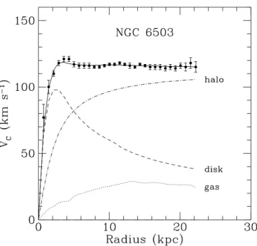
The Dark Matter puzzle is quite an old problem. In 1933, Zwicky, studying Hubble’s observations of the Coma Cluster of galaxies and assuming the validity of Newtonian Gravity, found that single galaxies were moving too fast for the cluster to remain bound together. As a possible solution to the problem, he postulated the existence of an unobserved type of mass, that he called dunkle Materie (Dark Matter)(see [17] for translation of the original paper). In the 1970s, another solid evidence was presented. Vera Rubin’s measurements of galaxy rotation curves [18], showed that the total mass of galaxies increased significantly with radius, even though very little additional stellar mass was present at these larger radii. A rotation curve is a plot of the circular velocity of stars or gas as a function of their distance from the galactic center. Denoting with r the distance from the centre of rotation, according to Newtonian gravity the velocity v(r) should scale as
v(r) = r
G
NM (r)
r , (1.1)
where M(r) = 4π
r
R
0
d r ˜ r ˜
2ρ(˜ r) and ρ(r) is the mass density profile of the galaxy. Consequently, beyond the optical disc one would expect that v(r) ∝ 1/ √
r. However, according for example to Figure 1.1, v(r) becomes approximately constant for large radii, meaning that M (r) ∝ r and ρ(r) ∝ 1/r
2. This feature cannot be explained by luminous matter, as Vera Rubin first noticed. Lastly, another strong evidence for DM comes from gravitational lensing, i.e. from deflection of light [20]. It is found by measurements to be much bigger compared to the one which could be produced by luminous matter.
If the reader was particularly interested in the history of DM, a comprehensive history can be found at [21].
Nowadays, analyzing PLANCK data (2018) [22] we know with very good precision the energy
1.1. DARK MATTER
Figure 1.1: Rotation curve of the galaxy NGC 6503. The dotted, dashed and dash-dotted lines are the contri- butions of gas, disk and dark matter, respectively. (Image Credit: [19]).
content of the universe. Roughly 27% of it, is estimated to be made of Dark Matter, compared to the 5% of ordinary matter, as shown in Figure 1.2. As mentioned in the introduction, DM behaves like dust, i.e. as an ideal fluid with equation of state of matter. However, to good accuracy, it seems to be collisionless and non-dissipating, properties which ordinary matter does not possess. For a detailed summary of the properties, bounds and models of DM, see [23, 24].
For the rest of the Chapter, the gravitational Newton constant G
Nis set to: G
N= 1 . The appropriate units are restored explicitly when necessary.
Figure 1.2: Estimated matter-energy content of the universe (Image: E. Ward/ATLAS Collaboration, Credit:
ESA and the Planck Collaboration).
1.2. IDEAL FLUID IN A HOMOGENEOUS UNIVERSE
1.2 Ideal Fluid in a Homogeneous Universe
We start now with the review of basics of Cosmology. A founding assumption of Cosmology, lies on the so called Cosmological Principle , which states that the universe on large scales is isotropic and homogeneous . Even though there are huge anisotropies at small scales, it has been found, that the distribution of galaxies becomes statistically homogeneous at scales larger than roughly 250 million light years.
Assuming isotropy and homogeneity of space of the universe, the metric can be written only in 3 non-equivalent ways as:
ds
2= dt
2− a(t)
2dr
21 − Kr
2+ r
2dΩ
2, (1.2)
where a(t) is called scale factor and K = {−1, 0, +1} corresponds to open, flat and closed universe, respectively. This metric is called FRLW-metric, after the names Alexander Friedmann, Georges Lemaître, Howard P. Robertson and Arthur Geoffrey Walker. The scale factor takes into account dilation or contraction effects on the whole space part of the metric. Its dynamic has to be derived from Einstein Equation:
R
µν− 1
2 g
µνR + Λ
cg
µν= 8πT
µν, (1.3) where T
µνis the energy-momentum tensor of the content of the universe. The matter/radiation is assumed to be an ideal relativistic fluid with energy density ρ and pressure p. The corresponding energy momentum tensor is given by [25]
T
µν= (ρ + p)u
µu
ν− pg
µν, (1.4)
where u
µis the 4-velocity of the fluid. The combination of 1.3 and 1.4 gives the following two equations, usually called Friedmann Equations , obtained from the 00 -component and from the trace of the ij - component:
a ˙ a
2+ K a
2= 8π
3 ρ + Λ
c3 ,
¨ a
a = − 4π
3 (ρ + 3p) + Λ
c3 .
(1.5)
To simplify them, the cosmological constant can be absorbed in both expression into p and ρ by redefining them. Therefore, in the following Λ
cwill be included in the other two parameters, reducing them to
a ˙ a
2+ K a
2= 8π
3 ρ , (1.6)
¨ a
a = − 4π
3 (ρ + 3p) . (1.7)
The ratio a/a ˙ is a measurable quantity, and is called Hubble Parameter , H . From Equation 1.6 and 1.7, it is possible to derive a third one related to the evolution of the energy density:
˙
ρ = −3H(ρ + p) , (1.8)
1.2. IDEAL FLUID IN A HOMOGENEOUS UNIVERSE
which shows how ρ changes due to the universe’s evolution. Assuming now a generic Equation of State p = w ρ , with w constant, Equation 1.8 can be solved resulting in:
ρ = ρ
Ia
Ia
3(w+1), (1.9)
where the subscript
Istands for the initial conditions. The cases of main interest are:
w =
0 ρ ∝ a
−3MATTER
1/3 ρ ∝ a
−4RADIATION
−1 ρ = const. "DARK ENERGY"
(1.10)
From the first Equation of 1.5, the geometry of the universe can be inferred:
K a
2=
8π
3 ρ − H
2. (1.11)
This motivates the definition of a critical energy density ρ
cas ρ
c≡ 3H
28π , (1.12)
so that
K a
2= 8π
3 (ρ − ρ
c) . (1.13)
Equivalently, people use often also the so called density parameter , Ω , which is defined as Ω ≡ ρ
ρ
c= 8πρ
3H
2, (1.14)
thus K
a
2= 8π
3 ρ
c(Ω − 1) . (1.15)
Therefore
K =
+1 ρ > ρ
cΩ > 1 CLOSED 0 ρ = ρ
cΩ = 1 FLAT
−1 ρ < ρ
cΩ < 1 OPEN
(1.16)
The most accurate measurement of these parameters have been obtained recently from the analysis of the Cosmic Microwave Background (CMB) by PLANCK in 2018. The result confirmed that Ω ≈ 1 , which means that the observable universe is essentially flat. A very detailed list of such values is given in [22]. Due to uncertainty in the measurements on the present Hubble parameter, H
0, cosmologists used to parametrize it with a constant h , which is typically in the range 0.4 < h < 1 , and write H
0= 100h
h
km s Mpci . The value that will be the most relevant for this thesis is of course the density parameter of Dark Matter, which is estimated to be
H
0= (67.4 ± 0.5) km
s Mpc
, Ω
DMh
2= 0.120 ± 0.001 . (1.17)
1.3. EQUILIBRIUM THERMODYNAMICS IN A HOMOGENEOUS UNIVERSE
1.3 Equilibrium Thermodynamics in a Homogeneous Universe
Before dealing with the dynamics of particles it is helpful to understand how a thermodynamical system of particles behave. A more general discussion can be found in [15]. The macroscopic parameters of interest are the number density n , the energy density ρ , and pressure p . All these parameters can be computed by integrating over the phase phase distribution. Since by assumptions the universe is homogeneous, the distribution cannot depend on the position, but only on the momentum p . Denoting with f(p) such a distribution and with g the number of degrees of freedom of the particle species of interest, then
n ≡ g (2π)
3Z
d
3p f(p) , ρ ≡ g
(2π)
3Z
d
3p E(p)f(p) , p ≡ g
(2π)
3Z
d
3p |p|
23E f (p) ,
(1.18)
where the energy E follows the relativistic relation E(p) = p
|p|
2+ m
2. As can be seen, for m = 0 the Equation of State of radiation, ρ = 3p , follows trivially. In general, describing the evolution of the phase space distribution out of thermal equilibrium is hard. To do that, the Boltzmann Equation is necessary and it will be treated in Section 1.4. Therefore, let us analyze first what happens in thermal equilibrium. In this case, we know from Statistical Mechanics that the phase space distribution of a system in thermal equilibrium at temperature T with chemical-potential µ is given by Bose-Einstein (- , bosons) and Fermi Dirac (+ , fermions) distributions:
f
eq(p) = 1 e
E−µT∓ 1
. (1.19)
In the non-relativistic limit E ≈ m and T m . Consequently, both Bose-Einstein and Fermi-Dirac distributions are approximated by the Boltzmann distribution:
f
eq(p)
Tm= e
−E−µT. (1.20)
The chemical potential of bosons must satisfy µ
boson≤ m , while it is unbounded for fermions. Equilib- rium with respect to the reaction a
1+ a
2+ · · · a
n−→ b
1+ b
2+ · · · b
mimposes the following condition on the chemical potential of the participating particles
n
X
i=1
µ
ai=
m
X
i=1
µ
bi. (1.21)
Consequently, chemical potentials are very closely related to number density asymmetries between
particles. If we are studying our model at temperatures bigger than GeV and taking into account
the observed particle-antiparticle asymmetries, they can be set to 0. There is no closed solution for
the integrals of Equation 1.18, but they can be computed in the approximation of relativistic and
1.3. EQUILIBRIUM THERMODYNAMICS IN A HOMOGENEOUS UNIVERSE
non-relativistic regime. In the relativistic case, i.e. T m:
n =
ζ(3)
π2
gT
3BOSE
3 4
ζ(3)
π2
gT
3FERMI ρ =
π2
30
gT
4BOSE
7 8
π2 30
gT
4FERMI p = 1
3 ρ ,
(1.22)
where ζ is the Riemann ζ -function. In the non-relativistic case, i.e. T m , fermions and bosons are described by the Boltzmann distribution shown in Equation 1.20 and hence there is no thermodynam- ical difference:
n = g mT
2π
3/2e
−m−µT, ρ = mn ,
p = nT .
(1.23)
In a radiation-dominated universe, it is clear from the above relations that the biggest contribution to the energy density (and pressure) comes from the relativistic species. Therefore, the total energy density is given by
ρ
R= π
230
g
∗T
4p
R= 1
3 ρ
R. (1.24)
where g
∗is the effective number of degrees of freedom of the relativistic species, i.e. those species with masses m
iT, which is given by
g
∗(T) = X
i∈bosons
T
iT
+ 7
8 X
i∈fermions
T
iT
. (1.25)
As can be seen, g
∗is a function of the temperature. As the universe expands and cools down, more particle species become non-relativistic and g
∗decreases. If the temperature is well above 100 GeV, all SM particles are relativistic and g
∗= 106.75 . Therefore, above 100 GeV, if we suppose that no unknown particle gets non-relativistic, g
∗is constant. For this reason, most of the universe history is dominated by radiation-like species. Using Equation 1.6 we get the Hubble parameter as a function of the temperature
H
R(T ) = 1.66 g
∗1/2T
2. (1.26) Another relevant quantity is the entropy density s ≡ S/V . This quantity can be related to the ones already mentioned as
s = ρ + p − µn T ≈ 2π
245 g
∗sT
3, (1.27)
where, as before, g
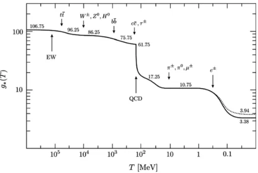
∗sis the entropic effective number of degrees of freedom. As can be seen from Figure
1.3, for most of the universe’s history, g
∗and g
∗shad the same values. However, if some species decouple
and they are still relativistic (e.g. neutrinos), then, they will still contribute to the total energy and
entropy density, but since they are decoupled their entropy density will be conserved separately.
1.4. THE BOLTZMANN EQUATION
Figure 1.3: Effective number of degrees of freedom, g
∗(solid line) and g
∗s(dotted line). (Image credit: Daniel Baumann, "Lectures Notes on Cosmology"[26]).
1.4 The Boltzmann Equation
Now that we have all the tools necessary to analyze the problem, we can start looking at the interaction of particles. What we are interested in is mainly the number density of DM, that is its abundance. To understand how the particle interactions influence this, the Boltzmann Equation is the key element.
1.4.1 The Boltzmann Equation
A more complete discussion can be found at [27]. The Boltzmann Equation (BE) describes the evolution of the phase space distribution of a system. The phase-space distribution f (t, x, p) for a given particle species indicates the number of particles dN within a volume of the phase space d
3x d
3p at a given time t , i.e.
dN = f (t, x, p) d
3xd
3p (1.28)
The evolution of f follows the equation
L[f ˆ ] = ˆ C[f ] , (1.29)
where L ˆ is the Liouville operator , which describes how f evolves in the phase-space and in time, and C ˆ is the collision term , which describes the change of f due to the collision (annihilation, creation, scattering) of the relative particle species with others. If we suppose to deal with a system of non- interacting particle, C ˆ is clearly 0, since their phase-space distribution will not change. It can be shown [27], that in the general relativistic scenario, the Lioville operator takes the following form:
L ˆ = p
µ∂
∂x
µ− Γ
µαβp
αp
β∂
∂p
µ, (1.30)
where Γ
µαβis the Christoffel symbol.
1.4. THE BOLTZMANN EQUATION
1.4.2 The Integrated Boltzmann Equation in Flat FLRW Universe
We are going to look at the Liouville operator and at the collision term separately. Since we are assuming homogeneity and isotropy, f can depend only on time and energy, i.e. f (t, E ) . Furthermore, we are more interested in the particle density n rather than in f itself. For this reason, it is convenient to integrate the BE over the phase space and study
g (2π)
3Z
d
3p L[f ˆ ] = g (2π)
3Z
d
3p C[f] ˆ . (1.31)
Considering the FRLW metric of a flat universe and Equation 1.30, L ˆ is found to be L ˆ
F RLW= E ∂
∂t − H|p|
2∂
∂E . (1.32)
Taking into account that n =
(2π)g 3R d
3p f(t, E) , the integrated Liouville term reduces to g
(2π)
3Z
d
3p L[f ˆ ] = ˙ n + 3Hn , (1.33) where we have introduced the notation
dndt≡ n ˙ . This is just the conservation of the number of particles.
We now consider the integrated collision term:
g (2π)
3Z
d
3p C[f ˆ ] . (1.34)
This term depends on the processes involved in the creation/annihilation of our particle species. Con- sider for example a 2-2 scattering: every particle that appears is described by a distribution f
i. The reaction is
1 + 2 −→ 3 + 4 . (1.35)
The integrated collision term for f
1is given by:
g (2π)
3Z
d
3p
1C[f ˆ
1] = − X
spins
Z
f
1f
2(1 ± f
1)(1 ± f
2)| M
12→34|
2−f
3f
4(1 ± f
3)(1 ± f
4)| M
34→12|
2(2π)
4δ(p
1+ p
2− p
3− p
4) dΠ
1dΠ
2dΠ
3dΠ
4,
(1.36)
where | M |
2is the squared amplitude probability of the process, (1 ± f
i) are the Pauli blocking/Bose enhancement factors ( ± for bosons/fermions) and dΠ
iis the invariant phase space volume given by
dΠ
i≡ d
3p
i(2π)
32E
i. (1.37)
The above equation generalize straightforwardly to other processes. Since 3-body (or more) interactions are much rarer then a 2-body interaction, in the following we are going to consider processes of the type:
a + b −→ 1 + 2 + 3 + . . . . (1.38)
1.4. THE BOLTZMANN EQUATION
The differential cross section is given by dσ ≡ dw
abT Φ = 1 4v
abE
aE
b| M
ab→...|
2(2π)
2δ(p
a+ p
b− X
i
p
i) Y
i
dΠ
i, (1.39)
where dw
abis the transition probability, T the time interval of the reaction, Φ is the flux of the particle and v
abis the relative velocity defined as
v
ab≡ q
(p
a· p
b)
2− m
2am
2bE
aE
b. (1.40)
We define the thermally averaged cross section as:
hσ
abv
abi =
R d
3p
ad
3p
bf
eq,af
eq,bσv R d
3p
ad
3p
bf
eq,af
eq,b=
R d
3p
ad
3p
bf
eq,af
eq,bσv
n
a,eqn
b,eq. (1.41)
Now we make four assumptions :
1. We assume Time Reversal symmetry , i.e. the reaction in one direction has the same probability to occur of the inverse one:
| M
ab→...|
2= | M
···→ab|
2≡ | M |
2. (1.42) 2. We neglect Pauli blocking/Bose enhancement factors for all particles:
(1 ± f ) ∼ = 1 . (1.43)
3. The produced particles interact strongly with the environment and are therefore in thermal equilibrium :
f
i−→ f
eq,i. (1.44)
4. For all particles, f
ican be approximated by the Boltzmann distribution , instead of using Bose- Einstein or Fermi-Dirac distribution:
f
eq,i= e
−Ei/T. (1.45)
These assumptions have an important consequence: since conservation of energy is ensured, we have
Y
i
f
i∼ = Y
i
f
eq,i= e
−P
i
Ei
/T
= e
−(Ea+Eb)/T∼ = f
eq,af
eq,b. (1.46) We conclude that:
Y
i
f
i∼ = f
eq,af
eq,b. (1.47)
This is referred to as principle of detailed balance . At this point we can simplify our calculations. We
consider the amplitude for an unpolarized process. Using the previous assumptions, it can be shown
1.4. THE BOLTZMANN EQUATION
that:
g (2π)
3Z
d
3p
aC[f ˆ
a] = − X
spin
Z "
f
af
b| M
ab→(...)|
2− Y
i
f
i| M
(...)→ab|
2#
(2π)
4δ(p
a+ p
b− X
i
p
i) dΠ
aΠ
bY
i
dΠ
i= − hσ
abv
abi [n
an
b− n
a,eqn
b,eq] .
(1.48)
If we assume that a = b, i.e. we consider the scattering of identical particles, then n
a= n
b≡ n. We conclude that for a process a + a → (. . . ) we have:
g (2π)
3Z
d
3p C[f ˆ ] = − hσvi
n
2− n
2eq. (1.49)
Thanks to the previous calculations we have the integrated BE:
˙
n + 3Hn = − hσvi
n
2− n
2eq. (1.50)
It can be shown [28], that under the previous approximations:
hσvi = 1
8m
4T K
22(m/T )
∞
Z
smin
σ(s)(s − 4m
2) √ s K
21√ s/T
, (1.51)
where K
n(z) is the n th K-Bessel function.
1.4.3 The Yield
In the following we write the integrated BE found in Equation 1.50 in term of the so-called Yield , defined as
Y ≡ n
s , (1.52)
where s is the entropy density. The advantage of this quantity is that it is conserved in the expansion, since both n and s depend in the same way on the scale factor. Now we assume the production of entropy to be negligible in time, i.e.
dS dt
∼ = 0 . (1.53)
This is a good approximation if the system is close to thermal equilibrium. Defined the entropy density s as S/a
3, this implies that:
s ˙ + 3H s = 0 (1.54)
and consequently
˙
n + 3Hn = ˙ Y s . (1.55)
It is more convenient to use the temperature as variable instead of time. This correspondence can be achieved through the Einstein equation for the conservation of energy, namely:
˙
ρ = −3H(ρ + p) . (1.56)
1.5. THE FREEZE-OUT MECHANISM
We write the equation of state p = wρ and, since in a radiation-dominated universe the energy density is mainly dominated by radiation, we set w = 1/3 . Lastly, we change variable from the temperature T to the dimensionless ratio m/T ≡ x and use ρ = π
2/30g
∗T
4. Using the previous considerations and defining the interaction rate
Γ ≡ n
eqhσvi , (1.57)
we get
Y
eqdY
dx = −x Γ(x) H(m)
Y
2− Y
eq2. (1.58)
Expressing the entropy density through Equation 1.27, we find the more practical equation dY
dx = −λ hσvi x
2Y
2− Y
eq2, (1.59)
with λ , restoring hidden natural units, given by λ ≡ 2π
245 g
∗s1.66 g
∗1/2M
P lm ≈ 0.26 g
∗sg
1/2∗M
P lm . (1.60)
1.5 The Freeze-Out Mechanism
The interesting feature of Equation 1.58 is that it depends on the ratio
HΓ. Basically this means that if H & Γ, i.e. if the interaction rate is smaller than the expansion rate of the universe, the term on the r.h.s. becomes small and eventually negligible, freezing the number density. As we have seen, if we have some particles in thermal equilibrium they follow the Bose-Einstein or Fermi-Dirac distribution. In the early universe it is reasonable to think that all the particles were in thermal equilibrium. However, if these particles are massive and remain in equilibrium as the temperature drops, their thermal distribution will start approaching a Boltzmann distribution, meaning that their number density will become exponentially suppressed as e
−m/T. It follows that for a massive particle species to have a relic density today, is crucial to get out of thermal equilibrium at a certain point.
These considerations lead to one of the main mechanisms to produce relic densities: the freeze-out . The main idea is the following. We start in the early universe at very high temperatures with a huge abundance of DM in thermal equilibrium with the other species. As the temperature drops below the mass of the DM particle, it starts to annihilate into lighter species. Eventually, the interaction rate of annihilation becomes smaller than the expansion rate of the universe leading the process to stop, freezing-out the number of particles. This mechanism is summarized in Figure 1.4.
Another option is that in the early universe some particle species were present in very small abundance and have never been in thermal equilibrium. The small abundance makes more likely for them to be produced than annihilated, increasing its abundance until H & Γ . This mechanism is referred to as freeze-in . It will not be considered here. To work, it requires in fact a very feeble interaction, i.e. a much weaker coupling compared to the range we are interested in.
One point has still to be discussed, namely if the DM decouples when it is still relativistic (hot-DM,
HDM) or not (cold-DM, CDM). The main difference between HDM and CDM can be found in structure
formation of galaxies. Simulation of DM has shown that if DM was hot, then the number of small
galaxies should be much smaller than the one actually observed. On the other hand, CDM manage to
1.5. THE FREEZE-OUT MECHANISM
Figure 1.4: Schematic illustration of the freeze-out mechanism (Image credit: Daniel Baumann, "Lectures Notes on Cosmology"[26]).
reproduce very well the process of structure formation. Nowadays, the HDM paradigm is considered to be ruled out and the CDM paradigm to be the most promising one. There is also the possibility of warm-DM (WDM), where the DM particle is assumed to be "mildly" relativistic. This hypothesis has not been ruled out and is still currently being studied. In the following, DM is assumed to be cold.
1.5.1 Freeze-Out of Non-Relativistic Species
Let us try to derive a rough approximation for the freeze-out following the approach of [29]. The starting point is the BE derived previously. Let us define the quantity ∆
Y≡ Y − Y
eq. We have two areas of interest: when x x
fand x x
f, where the subscript
fstands for the freeze-out point.
• x x
f: in this region, it is reasonable to assume that Y ≈ Y
eq. It follows that Y
2− Y
eq2= 2Y
eq∆
Y+ O (∆
Y)
2. Furthermore we can approximate
dYdx≈
dYdxeq≈ −Y
eq(use non-relativistic expression for n and the expression for s ). Then,
∆
Yf≈ x
2f2λ hσvi . (1.61)
• x x
f: since Y
eqfollows a Boltzmann distribution, we can assume that Y Y
eqand hence
∆
Y≈ Y . The equation then becomes d∆
Ydx ≈ − λ hσvi
x
2∆
2Y, (1.62)
which can be integrated to obtain the solution. Since the particles are now non-relativistic,
we can expand hσvi in powers of the velocity v or, alternatively, in inverse powers of x as
1.5. THE FREEZE-OUT MECHANISM
hσvi = a +
xb+ O(x
−2). Assuming that the value of x today, x
0, is much bigger of x
f, the previous equation gives
1
∆
Y0≈ 1
∆
Yf+ λ x
fa + b
2x
f. (1.63)
Now, the term ∆
Yfcan be ignored if one is not looking for very a precise result. This can be in principle checked using the result found previously. The freeze-out temperature can be estimated in a similar fashion and simulation shows that its value is about x
f≈ 20 , being not much sensitive to changes in the mass of the particle candidate. With this in mind, it follows
Y
0≈ ∆
Y0≈ x
fλ
a +
2xbf
. (1.64)
Denoting with Y
0and s
0the present values of the yield and of the entropy density, the relic density parameter is given by
Ωh
2= m Y
0s
0h
2ρ
c≈ 3 · 10
−27a +
40bcm
3s
. (1.65)
This result is feebly sensitive to the mass of the particle, which enters indirectly only through a, b . The correct DM relic density can be obtained if hσvi ≈ 3 · 10
−26h
cm3 s
i . As shown in [30], the relation between Ωh
2and hσvi can be better approximated as
10
27hσvi Ωh
2=
( 2.0 + 0.3 log
1010
27hσvi
as a function of hσvi 2.1 − 0.3 log
10Ωh
2as a function of Ωh
2. (1.66) Therefore, the relic abundance of Ωh
2= 0.12 can be achieved if
hσvi
f≈ 2 · 10
−26cm
3s
. (1.67)
It is important to stress that these results are valid only if nothing physically "odd" happens, e.g.
resonances. If we are in a range of parameters where the resonances are peaked, then this formula
is unreliable and the full BE must be solved. Away from resonances or if the peaks are negligible
compared to the overall shape, this result can be trusted.
Chapter 2
The Randall-Sundrum Model
In this Chapter, the underlying theoretical framework is reviewed, namely the Randall-Sundrum model. Sections 2.1 and 2.2.1 are presented following the lines of [31].
2.1 The Model
If we consider the Lagrangian of the Standard Model including the Einstein-Hilbert part for gravity, there are only two dimensionful parameters:
1. the Higgs expectation value, v ∼ = 246 GeV;
2. the Planck mass, M
P l≡ q
~cG
∼ = 1.22 · 10
19GeV.
In the end of the 90s a new idea was put forward, namely that the huge difference between these two values is not the consequence of a hierarchy in the Lagrangian’s parameters, but a consequence of the spacetime structure, in particular of extra-dimensions. The Randall-Sundrum is one of the models that originated [5].
This model is based on the following assumptions:
1. a 5th dimension compactified on S
1/Z
2; 2. 4D Lorentz invariance;
3. all dimensionful parameters are of the order of M
P l; 4. only gravity is 5-dimensional.
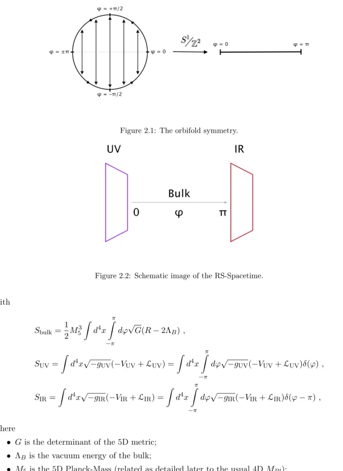
The above compactification goes under the name of orbifold symmetry and can be visualized in Figure 2.1. Considering the orbifold symmetry we localize the SM-fields at the fixed points, which correspond to 4D-subspaces ϕ = 0 and ϕ = π (or 0 and r
cif we define y = r
cϕ ). They are called respectively, UV-brane and IR-brane . A schematic summary can be found in Figure 2.2.
2.1.1 The Action and the Randall-Sundrum Metric
The branes and the bulk have their own part in the total action. The bulk action is just the usual Einstein-Hilbert action in a 5D spacetime, while the branes’ part contains the branes’ vacuum energy densities, usually called brane tensions , and generic Lagrangian densities.
S = S
bulk+ S
UV+ S
IR, (2.1)
2.1. THE MODEL
Figure 2.1: The orbifold symmetry.
Figure 2.2: Schematic image of the RS-Spacetime.
with
S
bulk= 1 2 M
53Z d
4x
Z
π−π
dϕ
√
G(R − 2Λ
B) ,
S
UV= Z
d
4x √
−g
UV(−V
UV+ L
UV) = Z
d
4x
π
Z
−π
dϕ √
−g
UV(−V
UV+ L
UV)δ(ϕ) ,
S
IR= Z
d
4x √
−g
IR(−V
IR+ L
IR) = Z
d
4x
π
Z
−π
dϕ √
−g
IR(−V
IR+ L
IR)δ(ϕ − π) ,
(2.2)
where
• G is the determinant of the 5D metric;
• Λ
Bis the vacuum energy of the bulk;
• M
5is the 5D Planck-Mass (related as detailed later to the usual 4D M
P l);
• V
UVand V
IRare the vacuum energy densities;
• L
UVand L
IRare the Lagrangian densities of the 4D-subspaces laying on the two branes;
• g
UVµν= G
µν(x, ϕ = 0) and g
µνIR= G
µν(x, ϕ = π) .
Note that in the following capital latin (greek) tensor indices, e.g.
M,
N(
µ,
ν), are used to indicate
5D (4D)-indices, respectively. In principle, L
UVand L
IRcan be fixed arbitrarily. In the following,
the simplest assumption is taken, namely L
UV= 0 while L
IRis set to be the SM Lagrangian. We
could have decided to set the SM-Lagrangian to be the UV-one, but this option does not provide an
2.1. THE MODEL
interesting theory from a phenomenological point of view. In fact, it would generate in the 4D-EFT an infinite tower of massive KK-modes with coupling exponentially suppressed with respect to the massless graviton of GR [32].
To find the metric, the Einstein Equation must be solved. In this case:
√
G(R
M N− 1
2 G
M NR + G
M NΛ
B) = 1 M
53V
IR√ −g
IRg
IRµνδ
Mµδ
νNδ(ϕ − π) + V
UV√ −g
UVg
µνUVδ
µMδ
Nνδ(ϕ) , (2.3) where R , R
M Nand Γ
LN Mare the 5D Ricci Scalar, Ricci Tensor and Christoffel Symbol, respectively.
They are given by
R = G
M NR
M N,
R
M N= Γ
LM L,N− Γ
LM N,L+ Γ
LN PΓ
PM L− Γ
LLPΓ
PM N, Γ
LN M= 1
2 G
LP(G
P M,N+ G
P N,M− G
M N,P) .
(2.4)
4D-Poincaré invariance of the metric, requires the metric to be of the following form:
ds
2= e
−2σ(ϕ)η
µνdx
µdx
ν− r
2cdϕ
2, (2.5) where r
cis a dimensionful parameter of the theory, needed to match the dimensions. It can be roughly thought as the width of the 5th dimension since
l
5=
π
Z
0
| d s|
dxµ=0= r
cπ
Z
0
d ϕ = πr
c. (2.6)
The form of σ(ϕ) must be determined through Einstein Equation 2.3. Denoting ∂
ϕσ ≡ ∂
5σ ≡ σ
0and A ≡ A(ϕ) ≡ e
−σ(ϕ), the Ricci tensor and the Ricci scalar are found to be
R
55= −4(σ
00− (σ
0)
2) , R
µν= A
2r
c2η
µν((σ
00− 4(σ
0)
2)) , R = G
M NR
M N= − 1
r
2cR
55+ A
−2η
µνR
µν= 4
r
c2((2σ
00− 5(σ
0)
2)) .
(2.7)
Then, the 55-component of Equation 2.3 gives
6(σ
0)
2= −Λ
Br
2c. (2.8)
The trace of the µν -components instead gives
− 3σ
00+ 6(σ
0)
2= −Λ
Br
c2− r
cM
53(V
IRδ(ϕ − π) + V
UVδ(ϕ)) . (2.9) Using Equation 2.8 this reduces to
3σ
00= r
cM
53(V
IRδ(ϕ − π) + V
UVδ(ϕ)) . (2.10)
2.1. THE MODEL
Let us try to solve these two equations. Equation 2.8 gives
σ
0= ±
r −Λ
B6 r
c≡ ±kr
c, (2.11) where k was defined as
k =
r −Λ
B6 . (2.12)
It follows that Λ
B< 0, and therefore the Bulk is an anti-deSitter spacetime. To satisfy Equation 2.10, the solution must have kinks at ϕ = 0, π . Therefore, it is given by
σ(ϕ) = kr
c|ϕ| with σ(ϕ + 2π) = σ(ϕ) . (2.13) Furthermore, this implies a constraint on the branes’ vacuum energies:
V
UV= −V
IR= 6M
53k . (2.14)
V
UVand V
IRare constrained in order to get a flat 4D space time. This is a fine tuning of the model.
The RS-metric is given by
ds
2= e
−2krc|ϕ|η
µνd x
µd x
ν− r
c2d ϕ
2. (2.15) The e
−krc|ϕ|factor that appears in the metric is called warp factor and it will be denoted with A(ϕ) . A very useful coordinate for the 5th-dimension is given by y = r
cϕ , which eliminates the factors of r
c. In this new coordinate, the warp factor is written as A(y) ≡ A(ϕ(y)) . The adimensional quantity kr
cwill be often denoted as
kr
c≡ µ . (2.16)
2.1.2 Solution to the Hierarchy Problem
We discuss now one of the main features of this model, i.e. the solution to the so called gauge- gravity hierarchy problem. For this, let us consider the Higgs part of the SM-Action and denote with Φ the Higgs field and with v
5and λ
5the 5D-parameters of the Higgs potential.
S
SM⊃ S
Higgs= Z
d
4x √
−g
IR| {z }
e−4µπ
g
IRµν|{z}
e2µπηµν
∂
µΦ
†∂
νΦ − λ
52
Φ
†Φ − v
522
2
. (2.17)
The kinetic term has a prefactor of e
−2µπ. To remove it and to bring the Lagrangian in canonical form, the following field redefinition is necessary:
Φ −→ e
µπΦ , (2.18)
that results in the following action:
S
Higgs= Z
d
4x
"
η
µν∂
µΦ
†∂
νΦ − λ
52
Φ
†Φ − v
252 e
−2µπ 2#
. (2.19)
2.2. WEAK FIELD EXPANSION
Comparing it with the standard Higgs Lagrangian, we find the following relations:
λ
4= λ
5,
v
4= v
5e
−µπ. (2.20)
The 5D-VEV gets a suppression by the warp factor. To get the usual 4D-VEV, µ needs to be of O (10) . In fact, making a very rough estimation, v
5∼ M
P l∼ 10
16TeV and v
4∼ TeV, thus
µ ∼ − 1 π log
v
4v
5∼ − 1
π log 10
−16∼ 12 . (2.21)
Therefore in this model, the fact that v
4M
P lis a consequence of the structure of spacetime and is not due to a hierarchy between the parameters of the Lagrangian.
Since this main feature is obtained for roughly e
µπ∼ 10
16, in the following, we are always going to assume that e
µπ1 and write briefly µ 1 when this approximation is used.
2.2 Weak Field Expansion
We study now the particle content of the Lagrangian by perturbing the metric. In order to get a canonical action, we set the perturbation parameter, κ to
˜ κ ≡ 1
M
53/2, κ ≡ 2˜ κ = 2
M
53/2, (2.22)
such that
G
perturbedM N= G
M N+ κ h
M Nwith G
M N= e
−2(µ|ϕ|)η
µν0 0 −r
2c!
. (2.23)
Gauge redundancy due to coordinate transformations have to be taken into account to exclude un- physical degrees of freedom. This it is what is going to be discussed in the next section.
2.2.1 Gauge Redundancy and Physical Degrees of Freedom
It can be shown that not all the degrees of freedom of the 5D metric-perturbation h
M Nare physical. To see this, we can decompose the perturbation with respect to the 5th dimension as
h
M N≡ T
µνh
µ5h
5νh
55!
≡ h
µνV
µV
νS
!
, (2.24)
where here T, V, S stand for tensor, vector and scalar field, respectively. As will be seen, imposing
the orbifold symmmetry and chosing properly the gauge, only h
µν≡ T
µνand h
55≡ S contain the
relevant degrees of freedom, while V
µcan be chosen to be zero. Furthermore, the scalar component
can be made independent of the 5th dimension. The 4D component corresponds to a spin-2 excitation
that we call graviton . The 55-component corresponds to a spin-0 particle, that is the excitation of the
5D-width and is therefore called radion .
2.2. WEAK FIELD EXPANSION
2.2.1.1 Metric Transformation Under Infinitesimal Change of Coordinates
To manifestly see the gauge structure of the theory, it is necessary to study how the metric changes under an infinitesimal change of coordinates. This will induce a transformation on the perturbation, highlighting how an opportune choice of the coordinates can eliminate part of the fields, that is, their
"unphysical"-part.
We start with some coordinates x
Nwith associated metric G
M Nand make the following coordinates transformation:
˜
x
N= x
N+ ξ
N(x) = ⇒ ∂x
P∂ x ˜
M= δ
PM− ∂ξ
P∂ x ˜
M+ O (ξ
2) , (2.25) with ξ
N(x) some function infinitesimally smaller than x
N. Then:
G ˜
M N(˜ x) = ∂x
P∂ x ˜
M∂x
Q∂˜ x
NG
P Q(x) = (δ
PM− ξ
P,M+ O (ξ
2))(δ
QN− ξ
Q,N+ O (ξ
2))G
P Q(x) =
= G
M N(x) − G
M P(x)ξ
P,M+ G
M P(x)ξ
P,N+ O (ξ
2) .
(2.26)
On the other side, also
G ˜
M N(˜ x) = ˜ G
M N(˜ x(x)) = ˜ G
M N(x) + ˜ G
M N,P(x)ξ
P+ O (ξ
2) = ˜ G
M N(x) +G
M N,P(x)ξ
P+ O (ξ
2) . (2.27) Therefore
G
M N−→ G ˜
M N(x) = G
M N(x) − G
N P(x)ξ
P,M+ G
M P(x)ξ
P,N− G
M N,P(x)ξ
P+ O (ξ
2) . (2.28) In the context of the RS model, the perturbed metric is given by the sum of the background (BG) metric, γ
M N, and the perturbation h
M N:
G
M N= γ
M N+ h
M Nwith d s
2BG= e
−2ση
µνd x
µd x
ν− d y
2, (2.29) G
M N−→ G ˜
M N(x) = G
M N(x) − γ
N P(x)ξ
P,M+ γ
M P(x)ξ
P,N− γ
M N,P(x)ξ
P+ O (ξ
2) . (2.30) Note that all indices are raised and lowered with the BG-metric, since we are not interested in higher order corrections. Then, it is found that:
h
µν−→ ˜ h
µν= h
µν− (ξ
µ,ν+ ξ
ν,µ) + 2σ
0γ
µνξ
5h
µ5−→ ˜ h
µ5= h
µ5− (ξ
µ,5+ ξ
5,µ) − 2σ
0ξ
µh
55−→ ˜ h
55= h
55− 2ξ
,5. (2.31)
2.2.1.2 Orbifold Symmetry and Unitary Gauge
It is now possible to study what happens if we choose properly the coordinates. Before doing
that, the symmetry of the theory must be included in the discussion. Let us recall that the invariant
spacetime interval ds
2must be invariant under the orbifold symmetry: (x, y) −→ (x, −y). This
fixes the transformation properties not only of the tensorial, vectorial and scalar components of the
2.2. WEAK FIELD EXPANSION
perturbation (Eq. 2.24), but also of the infinitesimal coordinate transformation:
Orbifold Symmetry = ⇒
h
µν(x, y) = h
µν(x, −y) V
µ(x, y) = −V
µ(x, −y) S(x, y) = S(x, −y) ξ
µ(x, y) = ξ
µ(x, −y) ξ
5(x, y) = −ξ
5(x, −y)
. (2.32)
Furtherore, since the geometric structure that was orbifolded is a circle, this also implies that the coordinate perturbation must be periodic, i.e.
ξ
M(x, y + 2πr
c) = ξ
M(x, y) . (2.33) Now we can focus on the two main results, i.e. that ξ
Mcan be chosen such that S(x) and V
µ(x, y) = 0.
Let us start with S(x, y) and ξ
5since they have a very simple transformation. Let us choose:
ξ
5(x, y) = 1 4
y
Z
−y
d y h ¯
55(x, y) ¯ − y 4πr
cπrc
Z
−πrc
d y h ¯
55(x, y) ¯ . (2.34)
It satisfies the orbifold symmetry and, thanks to the last term, is also periodic. From this it follows that
S ˜ ≡ ˜ h
55= 1 2πr
cπrc
Z
−πrc
d¯ y h
55(x, y) ¯ , (2.35)
that is independent of y . This fixes ξ
5, but we can still choose ξ
µto get rid of V
µ. In fact, we can prove that such ξ
µexists:
V ˜
µ≡ h ˜
µ5= h
µ5− ξ
5,µ− (ξ
µ,5+ 2σ
0ξ
µ) = h
µ5+ ξ
5,µ− e
−2σ∂
5(e
2σξ
µ) = 0
!, (2.36) thus
e
2σ(h
µ5− ξ
5,µ) = ∂
5(e
2σξ
µ) . (2.37) This has the solution
ξ
µ(x, y) = e
−2σ
y
Z
0
![Figure 1.4: Schematic illustration of the freeze-out mechanism (Image credit: Daniel Baumann, "Lectures Notes on Cosmology"[26]).](https://thumb-eu.123doks.com/thumbv2/1library_info/3996850.1540201/26.892.173.719.86.475/figure-schematic-illustration-mechanism-daniel-baumann-lectures-cosmology.webp)