On Supersymmetric Dark Matter

arXiv:hep-ph/0012206v1 16 Dec 2000

Pavel Fileviez Perez

Diploma Course in High Energy Physics.

The Abdus Salam International Centre for Theoretical Physics (ICTP).

Strada Costiera 11, 34100 Trieste, Italy.

and

Max-Planck Institut f¨ ur Physik (Werner-Heisenberg-Institut)

F¨ohringer Ring 6, 80805 M¨ unchen, Germany.

Supervisor:

Prof. Manuel Drees

Physik Department, Technische Universit¨at M¨ unchen, James Frank Strasse, D-85748 Garching, Germany.

December 8, 2000

The extra particles provided by Supersymmetry(SUSY) appear as natural candidates for ex- otica such as the missing Dark Matter of the Universe.

The particle candidates for Dark Matter, and the basic elements of the minimal supersym- metric extension of the Standard Model are reviewed. The needed elements to compute the neutralino counting rate are given, considering new Yukawa loop corrections to the neutralino- neutralino-Higgs boson couplings when the neutralino is a Bino-like state.

Including the new loop corrections in the Bino limit, the counting rate is improved in a 20%

for several values of the soft breaking supersymmetric parameters.

1

Dissertation at the Diploma Course in High Energy Physics. ICTP. Trieste. Italy. December, 2000.

1 Introduction. 3

2 Particle Candidates for Dark Matter (DM). 5

2.1 Introduction. . . . 5

2.2 Neutrinos. . . . 7

2.3 WIMPs. . . . 7

2.4 Axions . . . . 8

3 The Minimal SUSY Extension of the SM (MSSM). 9 3.1 Introduction. . . . 9

3.2 Particles and their Superpartners. . . . 12

3.3 The General Structure of the MSSM Lagrangian. . . . 14

3.4 Neutralinos. . . . 16

3.5 Squarks. . . . 19

3.6 The Higgs Bosons in the MSSM. . . . 20

3.7 R-symmetry and its Implications. . . . 21

4 Applications of SUSY Theories to the Description of DM. 23 4.1 Introduction. . . . 23

4.2 Yukawa One-Loop Corrections to the Bino-Bino-Higgs Boson Couplings. . . . 23

4.3 Effective Interactions. . . . 30

4.4 The Counting Rate. . . . 35

5 Conclusions. 39

2

Introduction.

The Dark Matter (DM) problem is one of the most interesting problems in modern physics.

What is the Dark Matter composition? What is the DM energy density present in our Uni- verse? What are the DM Baryonic and Non-Baryonic components? These are questions without a clear answer.

From several estimates it is known that the DM constitutes the dominant mass density in our Universe, and hence is of vital importance for predicting the future of the Universe.

The DM problem establishes a very nice connection between Cosmology and Particle Physics, given the possibility of predicting new particle candidates using the well known Standard Model and its extensions. In the Standard Model, the possible DM candidate is the neutrino, while in the Minimal Supersymmetric Extension of the Standard Model (MSSM), the lightest supersymmetric particle (neutralino or sneutrino) appears as possible candidate. Many ex- periments are looking for DM candidates [1]. If one these experiments finds DM candidates, it will provide a very important hint to clarify some fundamental ideas, such as the presence of supersymmetry at the weak scale.

As the fundamental theory to break Supersymmetry (SUSY) spontaneously is not known, the prediction of SUSY models such as the MSSM depends of many free parameters introduced to break SUSY. For example in the MSSM the soft breaking terms are introduced and therefore we take many free parameters entering in the interactions and the mass spectrums in the model. In the MSSM, the neutralino considered in many cases the ligthest supersymmetric particle is defined as the combination of the neutral gauginos. Different limits can be obtained for this particle, depending of the relation between the soft breaking parameters entering in its mass matrix. In our case we will consider the neutralino in the Bino-limit as the Dark Mattter particle candidate.

In the present dissertation we will review the different particle candidates for Non-Baryonic Dark Matter: the Light Neutrinos, the Weakly Interacting Massive Particles (WIMPs) and

3

the Axions, and the basic elements of the Minimal Supersymmetric Extension of the Standard Model, such as the relation between particles and their superpartners, the general structure of the MSSM lagrangian including the soft breaking terms, the mass spectrums of Squarks, Neutralinos and Higgs bosons, and the R-symmetry, which is used to define the neutralino as a stable particle.

In the Chapter 4 we introduce the different effective interactions to compute the neutralino

counting rate when the neutralino is a Bino-like state. In this case with the objective of im-

prove the neutralino counting rate we consider new Yukawa loop corrections to the neutralino-

neutralino-Higgs boson couplings. Numerical results of the counting rate and the relic density

are showed for several values of the soft supersymmetric parameters, where we can appreciate

the increment of the counting rate when the new loop corrections are taking into account.

Particle Candidates for Dark Matter (DM).

2.1 Introduction.

The phrase Dark Matter signifies matter whose existence has been inferred only through its gravitational effects. Evidence for DM comes from different cosmological scales, from galatic scales of several kiloparsecs and clusters of galaxies (Megaparsecs) to global scales of hundreds of Mpc’s.

The most well known evidence of DM comes from measurements of rotational velocities v

(r) of spiral galaxies. In this case at distances r greater than the extent of the visible mass, one expects that v

(r) ∝ r

, however it remains constant. Therefore from this discrepancy, the existence of dark haloes is inferred to explain this effect.

From different analyses in cosmology it is well known that the evolution of our Universe depends on the matter-energy present. Usually one uses the quantity Ω = ρ/ρ

, where ρ is the average density of our Universe and ρ

the critical density. The critical density is given by ρ

= 1.9 × 10

h

g cm

, when the Hubble constant H

is parametrised as h = H

/(100 km s

Mpc

), the recent measurements of the Hubble constant give H

= 73 ± 6(stat) ± 8(syst) km s

Mpc

, so that 0.6 ≤ h ≤ 0.9.

An estimate of the total matter density can be made from fluctuations in the Cosmic Mi- crowave Background Radiation (CMBR). The current data gives Ω

≃ 0.8 ± 0.2, in agree- ment with Ω

≃ 1 predicted by models of cosmic inflation [2]. This can be compared with the average density of visible matter in the Universe.

The matter mass density may be derived from astronomical determinations of the average mass-to-light ratio M/L for various astrophysical objects (see for example ref. [3]):

5

Ω

= M L

L ρ

(2.1)

from the M/L ∼ (3 − 9)M

/L

ratio measured in stars, is possible estimate Ω

:

0.002h

≤ Ω

≤ 0.006h

(2.2) with upper value Ω

≃ 0.012

Also through measurements of X-ray emission in clusters of galaxies we can estimate the total matter density [2]:

Ω

≃ 0.4 ± 0.1 (2.3)

On the other hand, from analyses of Big Bang nucleosynthesis, comparing the observed abun- dances of H, He and Li, and taking into account the chemical evolution of the Universe due to stellar burning, one finds [2]:

0.008 ≤ Ω

h

≤ 0.04 (2.4)

where the upper limit in this case is Ω

≃ 0.1.

Note that from the previous evaluation we can conclude that the major part of matter in the Universe is not visible and some of this Dark Matter is not baryonic. Therefore we can define two categories: Baryonic Dark Matter, composed of baryons which are not seen, and Non-Baryonic Dark Matter, composed of massive neutrinos, or elementary particles which are as yet undiscovered, where the particles which comprise non-baryonic DM must have survived from the Big Bang, and therefore must be stable or have lifetimes in excess of the current age of the Universe.

Also a very important point is that for purposes of galaxy formation models, the Non-Baryonic Dark Matter is classified as hot or cold, depending on whether the DM particles were moving at relativistic or non-relativistic speeds at the time galaxies could just start to form.

Many candidates to describe the DM are known, ranging from the axions with m ≤ 10

eV = 9 × 10

M

, to black holes of mass M = 10

M

.

The main baryonic candidates are massive compact halo objects (MACHOs), these include brown dwarfs, Jupiters, stellar black holes remnants, white dwarfs, and neutron stars.

As for non-baryonic candidates, we have light neutrinos as a candidate to describe the hot

component, and to describe the cold part, we have axions and weakly interacting massive

particles (WIMPs). The axion is motivated as a possible solution to the strong CP problem,

while WIMPs are stable particles, which arise in extensions of the Standard Model, such as

heavy fourth generation Dirac and Majorana neutrinos, and in SUSY models the lightest

neutralino and sneutrino.

In the next sections we will describe some of the particles candidates for Non-baryonic DM.

2.2 Neutrinos.

In units of critical density, the cosmic mass density for massive neutrinos is estimated as:

Ω

h

=

X

i=1

m

93 eV

The observed age of the Universe together with the measured expansion rate yields Ω

h

≤ 0.4 so that for any of the three families [4]:

m

≤ 40 eV (2.5)

This limit is probably the most important astrophysical contribution to neutrino physics. In this case, neutrinos with a mass 4 eV ≤ m

≤ 40 eV could represent all the non-baryonic Dark Matter.

When we consider the low mass neutrinos as particle DM candidates, two problems are present: from the perspective of structure formation, neutrinos as hot dark matter would require topological defects such as cosmic strings to form small structures such as galaxies.

The second problem is well known from the phase space constraint, for example if the neutrinos are the DM of dwarf galaxies, m

must be few hundreds of eV, which violates the upper limit from the overall cosmic mass density of about 40 eV [4]. Therefore these neutrinos can not describe the haloes of dwarf galaxies. However there exists the possibility to consider other candidates, for example the neutralino [1].

2.3 WIMPs.

The weakly interacting massive particles (WIMPs) are particles with masses between 10GeV and a few TeV, and with cross section approximately weak strength. Their relic density is approximately given by:

Ω

h

≃ 0.1 pb c

h σ

v i (2.6)

where c is the speed of light, σ

is the total annihilation cross section of a pair of WIMPs

into SM particles, v is the relative velocity between the two WIMPs in their cms system, and

h . . . i denotes thermal averaging.

Since WIMPs annihilate with very roughly weak interaction strength, it is natural to assume that their interaction with normal matter is also approximately of this strength. This raises the hope of detecting relic WIMPs directly, by observing their scattering off nuclei in a detector.

Perhaps the most obvious WIMP candidate is a heavy neutrino, however a SU(2) doublet neutrino will have a too small relic density, if its mass exceeds a few GeV. Also, one has to require the neutrino to be stable. It is not obvious why a massive neutrino should not be allowed to decay. However in SUSY models with exact R-parity, the lightest supersymmetric particle (LSP) is absolutely stable. In this case we have the sneutrino and the neutralino as candidates. However the sneutrinos have a large annihilation cross section, their masses would have to exceed several hundred GeV for them to make a good DM candidate, this would be uncomfortably heavy for the lightest superparticle.

The neutralino still can make a good cold DM candidate [5]. It is well known that for very reasonable SUSY parameters the relic density is 0.1 ≤ Ω

_e

h

≤ 0.3, which is the currently preferred range to the total DM density.

In the next chapter we will analyze some properties of the neutralinos, such as masses and the different physical states.

2.4 Axions

Axions are hypothetical pseudoscalar bosons, introduced to solve the strong CP-problem of QCD using the Peccei-Quinn Mechanism [6]

The axion mass arises from its mixing with the π

: m

≃ 0.6 eV 10

GeV

f

(2.7) In units of the cosmic critical density one finds for the axionic mass density:

Ω

h

≃ 0.23 × 10

( f

10

GeV )

θ

F (θ

) (2.8) where θ

is related to the average initial value of the axion field and F (θ

) with F (0) = 1 encapsules anharmonic corrections to the axion potential.

With Ω

h

≃ 0.3 × 2

the mass of dark matter axions is found to be m

= 30 − 1000µeV,

astrophysics limit very important to take into account for future experiments[6].

The Minimal SUSY Extension of the SM (MSSM).

3.1 Introduction.

The Glashow-Weinberg-Salam Model or Standard Model (SM), describes with a very good precision all electroweak processes. It is based on gauge invariance under the symmetry group:

G

= SU (3)

× SU(2)

× U (1)

(3.1) and its partial spontaneous symmetry breaking. In table 1 we show all its constituents, the elementary fermions (quarks and leptons), the scalar Higgs boson, the gauge bosons, and their transformation properties under G

(using Q = T

+ Y /2). The lagrangian of the Standard Model has the following form:

L

= L

+ L

+ L

+ L

(3.2) The explicit form of the SM lagrangian is well known, for our objectives we will write explicitly only the expression of the Yukawa interaction of the third generation:

L

= h

(¯ t ¯ b)

Φb

+ h

(¯ t ¯ b)

iσ

Φ

t

+ h

(¯ ν

τ ¯ )

Φτ

+ h.c (3.3) where h

, h

, h

, t, b, ν

and τ are the Yukawa couplings for each quark and lepton, the top quark, the bottom quark, the τ neutrino and the τ lepton, respectively (with R or L chiral- ity). Note that we can write these terms using only one scalar field Φ, which after electroweak symmetry breaking can generate mass for all the quarks and leptons in the SM.

As was mentioned above, the standard model has an extremely economical Higgs sector, which

9

accounts for all the particle masses. Baryon (B) and Lepton (L) numbers are automatically conserved and it is an anomaly free Quantum Field Theory. However all is not perfect. At present there is no unambiguous direct experimental evidence for the Higgs boson. Moreover there are no answers to some fundamental questions such as: Could we explain the origin of parity and time reversal breaking? Could we unify the diferent gauge couplings? Could we explain the origin of the CP violation?

Another fundamental problem in the Standard Model is in the Higgs sector. There is nothing to protect the mass of the Higgs boson from quadratic divergences. To solve this problem we can introduce a new symmetry called supersymmetry (SUSY). SUSY is a symmetry that transforms fermions into bosons and vice versa [7].

Motivations for introducing SUSY are the Haag-Lopuszanski-Sohnius Theorem (SUSY is the most general symmetry of the S-matrix), and cancellation of the tachyon states in String Theory. However the best (the more realistic) motivation is introduce SUSY at the weak scale to solve the problem related with the Higgs mass protection.

Once SUSY is introduced we will have a superpartner for each particle in the Minimal Super- symmetry Standard Model, and one aditional Higgs and its superpartner are introduced [8].

Note that if SUSY is realized in Nature, it means that we have discovered only aproximately the fifty percent of all particles.

From experiments (e.g at LEP) we know that the selectron, the superpartner of the electron must have a mass at least 90 GeV, more than 5 orden of magnitude above the electron mass.

Therefore SUSY must be broken. This raises an additional fundamental problem: How can we break SUSY spontaneously? We know that when a symmetry is broken spontaneously we can keep the renormalizability and the unitarity of our model, but in this case we don’t know the fundamental theory to break SUSY spontaneously.

In the MSSM, SUSY is broken explicitly by introducing soft breaking terms in the lagrangian.

These terms are called soft because the quadratic divergences (mass protection for the Higgs boson) are still canceled, but SUSY is broken [9].

In the present chapter we will describe some properties of the MSSM, the mass spectrum of

the Neutralinos, Squarks and Higgs bosons, and the main implications of the R-symmetry

introduced in this model.

SU(3)

, SU (2)

, U (1)

Quarks:

u

d

L

c

s

L

t

b

L

(3

, 2

, 1/3) u

d

t

(3

, 1

, 4/3) d

s

b

(3

, 1

, − 2/3) where i = 1, 2, 3 (colors)

Leptons:

ν

e

L

ν

µ

L

ν

τ

L

(1

, 2

, − 1) e

µ

τ

(1

, 1

, − 2) Scalars:

Φ =

φ

φ

(1

, 2

, 1) Gauge bosons:

G

with a = 1..8 (8

, 1

, 0) W

with b = 1..3 (1

, 3

, 0)

B

(1

, 1

, 0)

T able 1. Standard Model P articles

3.2 Particles and their Superpartners.

In the MSSM, we add a superpartner for each SM particles in the same representation of the gauge group. In Table 2 we show the names of the superpartners. For example the superpartner of the top quark is called stop, of the photon the superpartner is the photino, and similarly for the other particles. However, in the Higgs sector we must add another new Higgs boson and its superpartner to write the Yukawa interactions needed to generate masses for all quarks and to obtain an anomaly free model.

T able 2. Names of superpartners.

Fermions ⇐⇒ Sfermions

(quarks, leptons) (squarks, sleptons)

s = 1/2 s = 0

Gauge Bosons ⇐⇒ Gauginos

(W

, Z, γ, gluons) (W ino, Zino, photino, gluinos)

s = 1 s = 1/2

Higgs ⇐⇒ Higgsinos

s = 0 s = 1/2

Usually we use the SUSY operators in the left-chiral representation, therefore it is con-

venient to rewrite the SM particles (Table 1.) in the left-chiral representation and define

the superpartners accordingly. This leads to the superfield formalism, which makes it easier

to construct SUSY invariant lagrangians [10] . In this case we must introduce for each SM

particle one superfield, which contains the SM particle, its superpartner and an auxiliary

unphysical field. In Table 3 we show the third generation of the SM particles, their super-

partners and the superfields needed to write our lagrangian. Note that we have an extended

Higgs sector and the color index is omitted.

T able 3. Content of the MSSM.

(only the third generation)

Superfields Vector Superfields

Bosonic Fields Fermionic Fields G

G

G

with a = 1..8 G ^f

(8

, 1

, 0) G

W

with b = 1..3 W ^g

(1

, 3

, 0)

G

B

B e (1

, 1

, 0)

Chiral Superfields Leptons

L L ^f

=

ν f

τ f

L

=

ν

τ

(1

, 2

, − 1)

τ τ ^f

τ

(1

, 1

, 2)

Quarks

Q ^g Q

= ^f t

b f

t

b

(3

, 2

, 1/3) T t ^f

t

(3

, 1

, − 4/3) B b ^f

b

(3

, 1

, 2/3) Higgs

H

H

H

g H

H g

!

(1

, 2

, − 1)

H

H

H

g H

g H

!

(1

, 2

, 1)

3.3 The General Structure of the MSSM Lagrangian.

We can divide the lagrangian of the minimal extension of the Standard Model into two fundamental parts, the SUSY invariant and the Soft breaking term:

L

= L

+ L

(3.4)

In general we can write the SUSY invariant term as:

L

= L

+ L

+ L

+ L

+

Z

d

θ W + h.c (3.5) Having specified the content of the MSSM in Table 3 (including only the third generation of matter fields), we have to define the different terms of the lagrangian. The term L

has the following form:

L

= 1 4

Z

d

θ[2T r(W

W

) + 2T r(W

W

) + W

W

] (3.6) with:

W

= − 1

4 D D exp( − G

) D

exp(G

) (3.7) G

=

X

a=1

λ

2 G

(3.8)

W

= − 1

4 D D exp( − G

) D

exp(G

) (3.9) G

=

X

b=1

σ

2 G

(3.10)

and

W

= − 1

4 D DD

G

(3.11)

where λ

and σ

are the Gell-Mann and Pauli matrices, respectively. The SUSY covariant derivatives D and D are used in the left chiral representation:

D

= ∂

∂θ + 2iσ

θ∂

(3.12)

and

D

= − ∂

∂θ (3.13)

The lagrangians for gauge interactions of leptons, quarks and the Higgs bosons are:

L

=

Z

d

θ d

θ L

exp(2g

G

+ g

Y

2 G

)L+

+

Z

d

θ d

θ τ

exp(2g

G

+ g

Y

2 G

)τ (3.14)

L

=

Z

d

θd

θQ

exp(2g

G

+ 2g

G

+ g

Y

2 G

)Q+

+

Z

d

θ d

θ T

exp(g

Y

2 G

− g

(λ

)

G

)T + +

Z

d

θ d

θ B

exp(g

Y

2 G

− g

(λ

)

G

)B (3.15) L

=

Z

d

θ d

θ H

exp(2g

G

+ g

Y

2 G

)H

+ +

Z

d

θ d

θ H

exp(2g

G

+ g

Y

2 G

)H

(3.16)

where g

, g

, g

are the SU(3), SU(2) and U(1) coupling constants, respectively. The Y

rep- resent the hypercharges of the different superfields.

We can write the superpotential as the sum of two terms, W = W

+ W

. The first conserves lepton (L) and baryon (B) numbers:

W

= ǫ

[ − µH

H

+ h

H

L

τ + h

H

Q

B + h

H

Q

T ] (3.17) where ǫ

is the antisymmetric tensor, µ the Higgs mass parameter and h

, h

and h

are the different Yukawa couplings. The term W

, which explicitly breaks L and B numbers, is:

W

= ǫ

[ − µ

H

L

+ λL

L

τ + λ

L

Q

B] + λ

BBT (3.18) In W

the first three terms break lepton number, while the last term breaks baryon number.

If both B and L were broken, the proton would decay very rapidly, therefore the products λ ∗ λ

and λ

∗ λ

must be very small. In the last section of the present chapter we will analyze the R-symmetry related with the L and B numbers conservation and its implications.

The soft breaking term is:

−L

= m

| H

|

+ m

| H

|

+ m

(H

H

+ H

H

)+

+ Q ^g

†

M

_e Q ^g

+ t ^f

m

_e

R

t f

+ b ^f

†

m

_e

R

b f

+ L ^f

†

M _e

L ^f

+ τ f

m

_e

R

τ f

+

− H

Q g

(h

A

) t ^f

− H

Q g

(h

A

) b ^f

− H

L f

(h

A

) τ f

+

+ 1

2 [M

B e B ^e + M

W g

W ^g

+ M

g f

g ^f

] (3.19) Note that in order to describe SUSY breaking we introduce many free parameters, and several terms have mass dimension less than 4 (super-renormalizable, but not SUSY invariant). Also the different mass terms considered lift the degeneracy between particles and their superpart- ners [11].

3.4 Neutralinos.

Once SU(2)

× U (1)

is broken in the MSSM, fields with different SU(2)

× U (1)

quantum numbers can mix, if they have the same SU (3)

× U (1)

quantum numbers, and the same spin.

The neutralinos are mixtures of the B, the neutral ^e W ^f and the two neutral Higgsinos. In gen- eral these states form four distinct Majorana fermions, which are eigenstates of the symmetric mass matrix [in the basis ( B ^e , W ^f , H ^g

, ^g H

)] [8]:

M

=



 

 

M

0 − M

cos β s

M

sin β s

0 M

M

cos β c

− M

sin β c

− M

cos β s

M

cos β c

0 − µ M

sin β s

− M

sin β c

− µ 0



 

  (3.20)

where s

= sin θ

and c

= cos θ

.

Note that the masses of the neutralinos are determined by the values of four parameters M

, M

, µ and tan β =

=

1i

. The neutralino mass term is given by:

− L

= 1

2 (ψ

)

M

ψ

+ h.c (3.21)

If we define the physical states as χ

= N

ψ

, the diagonal mass matrix is M

=N

M

N

. In the limit M

, M

, µ ≫ M

, we can diagonalize the mass matrix very easily pertubatively.

In this case the eigenstates and their masses are [12]:

Bino-like:

χ e

≃ B ^e + N

H g

+ N

H g

(3.22) where:

N

= M

sin θ

(M

cos β + µ sin β)

µ

− M

(3.23)

N

= M

sin θ

(M

sin β + µ cos β)

− µ

+ M

(3.24)

and mass:

m _e

1

≃ M

(3.25)

Wino-like:

χ e

≃ W ^f + N

H g

+ N

H g

(3.26) with

N

= M

cos θ

(M

cos β + µ sin β)

− µ

+ M

(3.27)

N

= M

cos θ

(M

sin β + µ cos β)

µ

− M

(3.28)

and mass:

m _e

2

≃ M

(3.29)

Higgsino-like:

χ e

≃

H g

− H ^g

√ 2 + N

B ^e + N

W ^f

√ 2 + N

H ^g

√ 2 (3.30)

where

N

= M

sin θ

(sin β + cos β)

( − µ + M

) (3.31)

N

= M

cos θ

(sin β + cos β)

(µ − M

) (3.32)

N

= − δ

cos 2θ

1 + sin 2θ (3.33)

and

m

_e

3

≃ µ(1 + δ

) (3.34)

δ

is:

δ

= M

(1 + sin 2β)

2µ [ sin

θ

(µ − M

) + cos

θ

(µ − M

) ] (3.35)

Higgsino-like:

χ e

≃ H ^g

+ H ^g

√ 2 + N

B e + N

W f

√ 2 + N

H g

√ 2 (3.36)

with

N

= M

sin θ

( − sin β + cos β)

(µ + M

) (3.37)

N

= M

cos θ

(sin β + cos β)

(µ + M

) (3.38)

N

= − δ

cos 2θ

1 − sin 2θ (3.39)

with

m

_e

4

≃ − µ(1 + δ

) (3.40)

δ

is:

δ

= M

(1 − sin 2β)

2µ [ sin

θ

(µ + M

) + cos

θ

(µ + M

) ] (3.41)

Usually the unification of the gauge couplings is assumed, in this case the parameter M

≈ 2M

. Therefore from this relation we can conclude that the Wino eigenstates never will correpond to the LSP particle.

Now if M

≪ M

< M

< µ the LSP will be a nearly pure Bino eigenstate, while if M

≪ µ < M

< M

the LSP is a linear combination of the Higgsino states. For more details of neutralino masses in the MSSM see [13].

3.5 Squarks.

After the electroweak symmetry breaking, several terms in the MSSM lagrangian contribute to the squarks mass matrices. Ignoring flavor mixing between sfermions, the mass matrices for the stop and sbottom squarks are [8]:

stop mass matrix:

M _e

t

=



 

 

 



m

+ M

e

Q

+ m

(

−

sin

θ

) cos 2β − m

(A

+ µ cot β)

− m

(A

+ µ cot β) m

+ m

e

+

m

sin

θ

cos 2β



 

 

 



(3.42)

sbottom mass matrix:

M _e

b

=



 

 

 



m

+ M

_e

Q

− m

(

−

sin

θ

) cos 2β − m

(A

+ µ tan β)

− m

(A

+ µ tan β) m

+ m

e

−

m

sin

θ

cos 2β



 

 

 



(3.43)

in the basis ( f ^e

, f ^e

). The physical states are defined as:

f e

= f ^e

cos θ

_e + f ^e

sin θ

_e (3.44) and

f e

= − f ^e

sin θ

_e + f ^e

cos θ

_e (3.45) Note the contributions of the different soft breaking parameters in the mass matrices.

3.6 The Higgs Bosons in the MSSM.

As we have mentioned before, the existence of the Higgs bosons is the main motivation to introduce SUSY at the electroweak scale. In the MSSM the tree-level Higgs potential is given by [9]:

V

= m

| H

|

+ m

| H

|

+ m

(H

H

+ h.c)+ (3.46) + g

+ g

8 ( | H

|

− | H

|

)

+ g

2 (H

H

)

(3.47) where m

= m

+ | µ |

with i = 1, 2

Note that in this equation the strength of the quartic interactions is determined by the gauge couplings.

After electroweak symmetry breaking, three of the eight degrees of freedom contained in the two Higgs boson doublets get eaten by the W

and Z gauge bosons. The five physical degrees of freedom that remain form a neutral pseudoscalar boson A

, two neutral scalar Higgs bosons h

and H

, and two charged Higgs bosons H

and H

. The physical pseudoscalar Higgs boson A

is a linear combination of the imaginary parts of H

and H

, which have the mass matrix[

in the basis (

,

]):

M

= − m

tan β − m

− m

− m

cot β

!

(3.48)

m

= trM

= − 2m

/ sin(2β) (3.49) The other neutral Higgs bosons are mixtures of the real parts of H

and H

, with tree-level mass matrix [

,

]:

M

= − m

tan β + m

cos

β m

−

m

sin 2β m

−

m

sin 2β − m

cot β + m

sin

β

!

(3.50)

In this case the eigenvalues are:

m

= 1

2 [m

+ m

± ^q (m

+ m

)

− 4m

m

cos

(2β)] (3.51) From this equation we can see that at tree level, the MSSM predict that m

≤ m

, unfortu- nately in this case when we consider one-loop corrections, the mass of the light Higgs boson is modified significantly. For example assuming that the stop masses do not exceed 1 TeV, m

≤ 130 GeV [14]. In this example we can see the importance of loop corrections in the computation of physical quantities.

3.7 R-symmetry and its Implications.

In the Standard Model the conservation of Baryon (B) and Lepton (L) number is automatic, this is an accidental consequence of the gauge group and matter content. In the MSSM, as we showed in the second section of this chapter, we can separate the most general gauge invariant superpotential basically into two fundamental parts, where the first term conserves B and L, while the second breaks these symmetries.

In the MSSM, B and L conservation can be related to a new discrete symmetry, which can be used to classify the two kinds of contributions to the superpotential. This symmetry is the R-parity, defined as:

R = ( − 1)

(3.52)

Quark and lepton supermultiplets have R = − 1, while the Higgs and gauge supermultiplets have R = +1. The symmetry principle in this case will be that a term in the lagrangian is allowed only if the product of the R parities is equal 1.

The conservation of R-parity as defined in equation (3.52), together with spin conservation, also implies the conservation of another discrete symmetry, defined such that it will be +1 for the SM particles and -1 for all the sparticles:

R

= ( − 1)

(3.53)

Now if we impose the conservation of R

, we will have some important phenomenological consequences:

• The lightest particle with R

= − 1, called the lightest supersymmetric particle (LSP), must be stable.

• Each sparticle other than the LSP must decay into a state with an odd number of LSPs.

• Sparticles can only be produced in even numbers from SM particles.

Applications of SUSY Theories to the Description of DM.

4.1 Introduction.

Two methods have been proposed to search for relic neutralinos [1]. The first is the direct detection, observing their scattering off nuclei in a detector. The second is to look for signals for ongoing neutralino annihilation. In the second case the idea is that the neutralino can lose energy in collisions with nuclei and can then be trapped by the gravitational field of celestial bodies, then eventually will become sufficiently concentrated near the center of these bodies to annihilate with significant rate. As is well known to analyze these possibilities, it is very important to know very well the neutralino-nucleon scattering cross section.

In this chapter, knowing the basic elements of the SUSY extension of SM, such as interactions and spectrum, and assuming the neutralino as the lightest supersymmetric particle [5], we will compute the counting rate in the limit where the neutralino is a Bino-like state. In this case we will include the one-loop corrections to the neutralino-neutralino-Higgs bosons couplings.

4.2 Yukawa One-Loop Corrections to the Bino-Bino- Higgs Boson Couplings.

As we mentioned in the previous chapter, we can obtain different limits for the neutralino physical states. One of the more interesting limits is the bino limit. In this case it is possible to compute with good precision the dark matter density contribution needed to describe the dark haloes in the spiral galaxies.

23

In this section we will analyze the LSP-LSP-Higgs bosons couplings in the Bino limit at one- loop level, with the objective of computing the counting rate in direct experiments.

At tree level these couplings vanish in the pure Bino limit, therefore we will consider the one-loop correction to the elastic cross section.

Using the Feynman Rules [15], the tree-level couplings are given by:

iΓ

e

e

= i(sin α N

− cos α N

)(g

N

− g

N

) (4.1) iΓ

e

e

= i(sin α N

+ cos α N

)(g

N

− g

N

) (4.2) iΓ

e

e

= γ

(sin β N

− cos β N

)(g

N

− g

N

) (4.3) Note that for the pure Bino state (only N

6 = 0) all these couplings are zero at tree level.

Here the Higgs mixing angle α can be obtained from the following expressions:

sin 2α = − sin 2β m

+ m

m

− m

(4.4) and

cos 2α = − cos 2β m

− m

m

− m

(4.5)

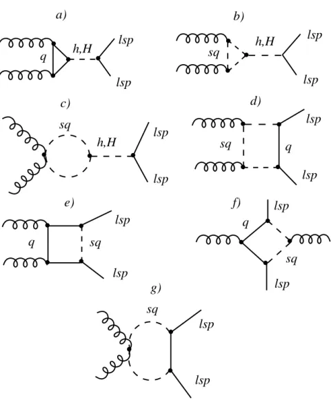
At one-loop level we will consider contributions which contain Yukawa interactions in the quark-squark loops. We therefore have to include heavy quarks and their superpartners inside the loops (see Fig 5.1). In this case the expressions for these couplings are given by:

- Scalar Higgs bosons h

and H

:

iδΓ

_e

e

= − 3i

8π

[h

δ

+ h

δ

]N

(4.6) where:

δ

= C

{

X

i=1

(a

_e

i

− b

_e

i

)[(m

_e

i

+ m

+ m

_e

χ⁰

)C

( q e

) − 4m

_e

χ⁰

C

( q e

)]

+2m

_e

m

X

i=1

(a

_e

i

+ b

_e

i

)[C

( q e

) − 2C

( q e

)] }

+

X

i,j=1

C _e

[m

(a _e

a _e

− b _e

b _e

)C

( q e

, q e

) + 2m

_e

(a _e

a _e

+ b _e

b _e

)C

( q e

, q e

)] (4.7) -Pseudoscalar Higgs boson A

.

iδΓ

_e

e

= − 3iγ

8π

[h

δ

+ h

δ

]N

(4.8) with:

δ

= C

{

X

i=1

(a

_e

i

− b

_e

i

)( − m

_e

i

+ m

+ m

_e

χ⁰

)C

( q e

) + 2m

_e

m

X

i=1

(a

_e

i

+ b

_e

i

)C

( q e

) } +

X

i6=j=1

C _e

[m

(a _e

b _e

− a _e

b _e

)C

( q e

, q e

) − 2m

_e

(a _e

b _e

+ a _e

b _e

)C

( q e

, q e

)] (4.9) Here C

, are the quark-quark-Higgs bosons couplings, while C _e

represents the q e

− q ^e

− Higgs bosons couplings: i, j labels the squark mass eigenstates.

The interaction quark-squark-neutralino is written as:

L

_e

_e

= q(a _e

+ b _e

γ

) χ ^f

q e

+ h.c (4.10) We are using the following notation for the loop integrals [16] (see appendix A):

C

( q e

) = C

(k

, k

, m

, m

_e

, m

) (4.11)

C

( q e

, q e

) = C

(k

, k

, m

_e

, m

, m

_e

) (4.12)

C

( q e

) = C

( − k

, k

, m

, m

, m

_e

) (4.13)

C

( q e

, q e

) = C

(k

, − k

, m

_e

, m

_e

, m

) (4.14)

C

( q e

, q e

) = C

(k

, − k

, m

_e

, m

_e

, m

) (4.15)

where k

represent the neutralino momentum. As already noted only consider the contribution

of heavy quarks and their superpartners in the loop (only the third generation quarks).

In the case of the top quark, using the Feynman rules given in [15] the parameters are:

Yukawa coupling:

h

= g

m

√ 2m

sin β (4.16)

and

a

_e

= g

tan θ

√ 2 ( − 1

6 cos θ _e

+ 2

3 sin θ _e

) (4.17)

a

_e

= g

tan θ

√ 2 ( 1

6 sin θ _e

+ 2

3 cos θ _e

) (4.18)

b

_e

= g

tan θ

√ 2 ( − 1

6 cos θ _e

− 2

3 sin θ _e

) (4.19)

b

_e

= g

tan θ

√ 2 ( 1

6 sin θ _e

− 2

3 cos θ _e

) (4.20)

the couplings for the heavy Higgs boson H

are given by:

t − t − H

C

= − sin α

√ 2 (4.21)

t e − ^e t − H

C _e

= − √

2[ m

sin β cos(α + β) m

cos

θ

( 1

2 cos

θ _e

− 2

3 sin

θ

cos 2θ _e

) + m

sin α − 1

2 sin 2θ _e

(µ cos α + A

sin α)] (4.22) C _e

= − √

2[ m

sin β cos(α + β) m

cos

θ

( 1

2 sin

θ _e

+ 2

3 sin

θ

cos 2θ _e

) + m

sin α + 1

2 sin 2θ _e

(µ cos α + A

sin α)] (4.23) C _e

= C _e

= − √

2[ − m

sin β cos(α + β) sin 2θ _e

4m

cos

θ

− 1

2 cos 2θ _e

(µ cos α + A

sin α)] (4.24)

In the case of the light Higgs boson the couplings are:

t − t − h

C

= − cos α

√ 2 (4.25)

e t − ^e t − h

C _e

= − √

2[ − m

sin β sin(α + β) m

cos

θ

( 1

2 cos

θ _e

− 2

3 sin

θ

cos 2θ _e

) + m

cos α + 1

2 sin 2θ _e

(µ sin α − A

cos α)] (4.26) C _e

= − √

2[ − m

sin β sin(α + β) m

cos

θ

( 1

2 sin

θ _e

+ 2

3 sin

θ

cos 2θ _e

) + m

cos α − 1

2 sin 2θ _e

(µ sin α − A

cos α)] (4.27) C _e

= C _e

= − √

2[ m

sin β sin(α + β) sin 2θ _e

4m

cos

θ

+ 1

2 cos 2θ _e

(µ sin α − A

cos α)] (4.28) For the contribution of the pseudoscalar Higgs boson A

, the couplings are:

t − t − A

C

= − i cos β

√ 2 (4.29)

t e − ^e t − A

C _e

= − C _e

= i sin β

√ 2 (µ − A

cot β) (4.30)

C _e

= C _e

= 0 (4.31) We now turn to the sbottom coupling.

The Yukawa coupling is:

h

= g

m

√ 2m

cos β (4.32)

and

a

_e

= g

tan θ

√ 2 ( − 1

6 cos θ _e

− 1

3 sin θ _e

) (4.33)

a

_e

= g

tan θ

√ 2 ( 1

6 sin θ _e

− 1

3 cos θ _e

) (4.34)

b

_e

= g

tan θ

√ 2 ( − 1

6 cos θ _e

+ 1

3 sin θ _e

) (4.35)

b

_e

= g

tan θ

√ 2 ( 1

6 sin θ _e

+ 1

3 cos θ _e

) (4.36)

The b − b − H

coupling is given by:

C

= − cos α

√ 2 (4.37)

and the couplings ^e b − ^e b − H

are:

C _e

= − √

2[ m

cos β cos(α + β) m

cos

θ

( − 1

2 cos

θ _e

+ 1

3 sin

θ

cos 2θ _e

) + m

cos α − 1

2 sin 2θ _e

(µ sin α + A

cos α)] (4.38) C _e

= − √

2[ m

cos β cos(α + β) m

cos

θ

( − 1

2 sin

θ _e

− 1

3 sin

θ

cos 2θ _e

) + m

cos α + 1

2 sin 2θ _e

(µ sin α + A

cos α)] (4.39) C _e

= C _e

= − √

2[ m

cos β cos(α + β) sin 2θ _e

4m

cos

θ

− 1

2 cos 2θ _e

(µ sin α + A

cos α)] (4.40)

In the case of the light Higgs boson h

the couplings are:

b − b − h

C

= sin α

√ 2 (4.41)

e b − ^e b − h

C _e

= √

2[ m

cos β sin(α + β) m

cos

θ

( − 1

2 cos

θ _e

+ 1

3 sin

θ

cos 2θ _e

) + m

sin α + 1

2 sin 2θ _e

(µ cos α − A

sin α)] (4.42) C _e

= √

2[ m

cos β sin(α + β) m

cos

θ

( − 1

2 sin

θ _e

− 1

3 sin

θ

cos 2θ _e

) + m

sin α − 1

2 sin 2θ _e

(µ cos α − A

sin α)] (4.43) C _e

b12

= C _e

b21

= √

2[ m

cos β sin(α + β) sin 2θ _e

4m

cos

θ

+ 1

2 cos 2θ _e

(µ cos α − A

sin α)] (4.44) The couplings of the pseudoscalar Higgs boson A

:

b − b − A

C

= i sin β

√ 2 (4.45)

e b − ^e b − A

C _e

= − C _e

= i cos β

√ 2 (µ + A

tan β) (4.46)

C _e

= C _e

= 0 (4.47)

4.3 Effective Interactions.

The neutralino-nucleus elastic cross section is of fundamental importance. It determines the detection rate in direct and indirect detection experiments.

In general the WIMP-nucleus elastic cross section depends fundamentally on the WIMP- quark interaction strength, on the distribution of quarks in the nucleon and the distribution of nucleons in the nucleus [1].

To compute the WIMP-nuclei interaction, we must first compute the interactions of WIMPs with quarks and gluons, after using the matrix elements of the quark and gluons operators in a nucleon state we compute the interaction with nucleons and finally using the nuclear wave functions, it is possible to compute the matrix element for the WIMP-nucleus cross section.

In the non-relativistic limit we have only two types of neutralino-quark interaction, the spin- spin interaction and the scalar interaction. In the case of spin-spin interaction, the neutralino couples to the spin of the nucleus, and in the case of the scalar interaction the neutralino couples to the mass of the nucleus.

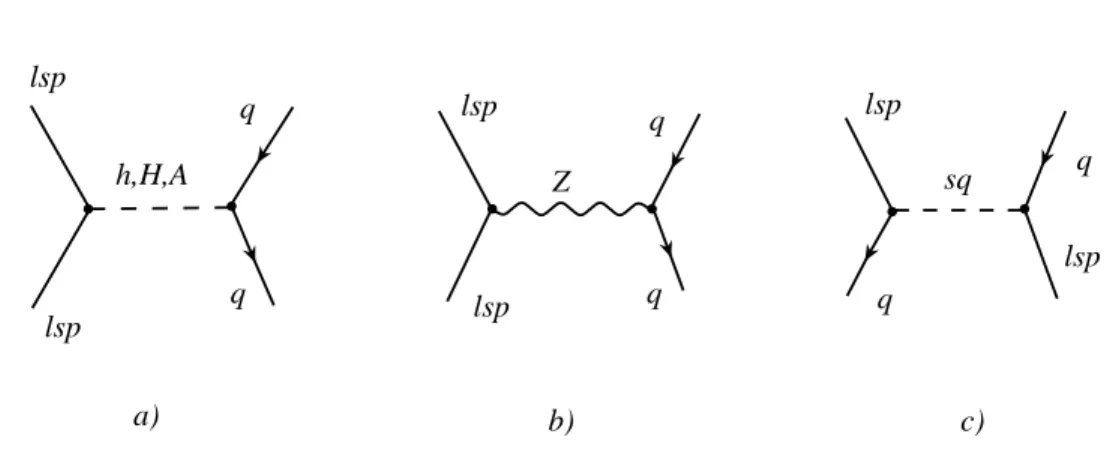
To start with the analysis of the neutralino-nucleus interaction, we can discuss the effective lagrangian describing the neutralino-quark interaction. In this case we have three classes of contributions, the exchange of a Z

or Higgs boson and squark exchange (Fig 5.2).

From the Z

and squark exchange we have spin-dependent contributions, while the Higgs and squark exchange contribute to the spin-independent interactions.

The spin-dependent contribution is [17]:

L

= χ ^f

γ

γ

χ f

qγ

(c

+ d

γ

)q (4.48) where:

c

= − 1 2

X

i=1

a

_e

b

_e

m

_e

i

− (m

_e

+ m

)

+ g

4m

O

(T

− 2e

sin

θ

) (4.49) d

= 1

4

X

i=1

a

_e

i

+ b

_e

i

m

_e

i

− (m

_e

+ m

)

− g

4m

O

T

(4.50)

The second term in c

and d

represents the Z

exchange, g

is the SU(2) gauge coupling, θ

the weak mixing angle, T

= ± 1/2 and e

the weak isospin and electric charge of the quark q, and O

=

(N

− N

) describes the Z

χ e

χ e

coupling.

To determine the spin-dependent neutralino-nucleon interaction, we must compute the matrix element:

h N | qγ

γ

q | N i = 2s

△ q

(4.51)