’t Hooft coupling

JHEP08(2019)006

Published for SISSA by Springer

Received : May 3, 2019 Revised : June 24, 2019 Accepted : July 22, 2019 Published : August 1, 2019

Quasinormal modes of magnetic black branes at finite

’t Hooft coupling

Sebastian Waeber

Institute for Theoretical Physics, University of Regensburg, Universit¨ atsstr. 31, D-93040 Regensburg, Germany

E-mail: sebastian.waeber@physik.uni-regensburg.de

Abstract: The aim of this work is to extend the knowledge about Quasinormal Modes (QNMs) and the equilibration of strongly coupled systems, specifically of a quark gluon plasma (which we consider to be in a strong magnetic background field) by using the duality between N = 4 Super Yang-Mills (SYM) theory and type IIb Super Gravity (SUGRA) and including higher derivative corrections. The behaviour of the equilibrating system can be seen as the response of the system to tiny excitations. A quark gluon plasma in a strong magnetic background field, as produced for very short times during an actual heavy ion collision, is described holographically by certain metric solutions to 5D Einstein-Maxwell- (Chern-Simons) theory, which can be obtained from type IIb SUGRA. We are going to compute higher derivative corrections to this metric and consider α ^{0 3} corrections to tensor- quasinormal modes in this background geometry. We find indications for a strong influence of the magnetic background field on the equilibration behaviour also and especially when we include higher derivative corrections.

Keywords: AdS-CFT Correspondence, Holography and quark-gluon plasmas, Black Holes in String Theory, Gauge-gravity correspondence

ArXiv ePrint: 1811.04040

JHEP08(2019)006

Contents

1 Introduction 1

2 Reviewing magnetic black branes in the λ → ∞ limit 3

3 Higher derivative corrections 6

3.1 A helpful prescription and its mathematical proof 8

3.2 An alternative algorithm to compute higher derivative corrections to the

AdS-Schwarzschild black hole solution 11

3.3 Calculating higher derivative corrections to the magnetic black brane metric 14 3.4 Approximating higher derivative corrections to tensor QNMs without mag-

netic background field 18

3.5 Approximating higher derivative corrections to the first tensor QNM in the

presence of a strong magnetic background field 20

3.6 Resumming finite λ corrections to the first tensor QNM in a strong magnetic

background field 24

4 Discussion 26

A Equation of motion of tensor fluctuations for b = 0 27

B Expansion coefficients 28

1 Introduction

The formalism to qualitatively describe the early, far from equilibrium dynamics of the QCD phase of high energy density (for which the term quark gluon plasma (QGP) will be used even in the non-thermalized state) generated during heavy ion collisions at RHIC or LHC is one of the most prominent applications of the gauge/gravity duality, more specifically of the duality between N = 4 super Yang-Mills theory (SYM) in 4 dimensions and supergravity (SUGRA) on AdS ₅ × S ₅ known as the AdS/CFT duality. In the weak formulation the gauge group rank N of the boundary theory is taken to infinity. The supergravity limit for the AdS/CFT correspondence in the case of N = 4 SYM theory holds within the parametric region 1 λ N and allows the description of far from equilibrium dynamics at strong coupling.

After having determined certain observables with the help of the holographic principle

an interesting next question would be how their higher derivative or α ⁰ -corrections behave

and how large they are. Computing finite ’t Hooft coupling corrections is notoriously messy

and involved, but necessary, if ones wishes to leave the unrealistic λ → ∞ limit.

JHEP08(2019)006

Within a formalism that helps to describe QGPs far from equilibrium a natural aspect that can be analyzed is how and how fast such a system equilibrates. At late times this question breaks down to the analysis of quasinormal modes (QNMs), fluctuations around the equilibrium state. The inverse of the absolute value of the imaginary part of QNM frequencies, which correspond to the poles of the propagator of such a fluctuation, is pro- portional to the equilibration time. Thus, the QNM with the smallest absolute imaginary part determines the time the system needs to equilibrate. The real part gives information about the energy of the mode, i.e. the frequency of the fluctuation.

Motivated by the work of [2], we are going to consider higher derivative corrections to the magnetic black brane metric and to tensor QNMs in a coupling corrected magnetic black brane background. The propagator of these perturbations h xy is dual to the two-point func- tion of the xy component of the boundary stress energy tensor. Our numerical analysis gave a well converging result for the lowest α ⁰ -corrected QNM frequency. The numerical errors of the α ⁰ -corrections to the higher QNMs were too large to give reasonable results for the parameters (size of the magnetic field, grid sizes for numerical methods etc.) we chose here. ¹ On the one hand we want to study how the late time behaviour of the QGP changes, if we consider it to be in a strong magnetic field, as produced for a very a short time during heavy ion collisions, and include higher α ⁰ corrections, to leave the λ → ∞ limit. On the other hand this analysis also has a more abstract application: so far, we don’t have a satisfying dual theory, that describes QCD. The most prominent AdS/CFT duality allows us to non-perturbatively compute quantities in a conformal field theory, with N → ∞ and λ = g _YM ² N → ∞ . Whereas QCD has a finite coupling, a finite N = 3 and is not conformally invariant. Apart from (bottom-up-) modeling, one should try everything that is feasible on the gravity side, to bring the dual field theory closer to QCD in a top-down fashion.

This includes the computation of finite coupling corrections, 1/N corrections, breaking the scale invariance e.g. by introducing a magnetic background field, where the metric ansatz describing this setting can be deduced from a solution to 10D SUGRA, or several of the above simultaneously.

In the limit λ → ∞ the holographic description of a QGP in a magnetic background field was realized in [2] by considering a Einstein-Maxwell-Chern-Simons theory. That this setting describes the physical properties of the real SU(3) QGP at least qualitatively was shown in [24]. In this work we will convince ourselves that the ansatz chosen in [2] can be derived from a specific solution to SUGRA living in 10 dimensions (see [26]). This allows us to determine α ⁰³ -corrections first to the metric of a magnetic black brane, where the mag- netic background field back-reacts to the geometry, and afterwards to QNM fluctuations

1

The tendency that higher modes are numerically more difficult to extract is not confined to this setting and already can be seen without having a magnetic background field and without having coupling correc- tions. The technical reason for this e.g. in the case of spectral methods is that the number of modes one can extract grows linearly with the size of the applied basis of spectral functions, where the lowest modes are already captured at rather modest orders, whereas higher modes need higher order procedures to converge.

The physical reason for this is that higher modes i.e. higher frequencies correspond to smaller length scales,

which are more difficult to resolve. The tendency that α

corrections addtitionally increase the difficulty

of numerically extracting higher modes already exists without a magnetic background field [17, 18]. A

magnetic background field of the size we chose in this paper (B ≈ 34.5T

) strongly enforced this tendency.

JHEP08(2019)006

around this specific solution. We are going to give a mathematical proof of a prescription, which was found in [18], to handle higher derivative corrections to the five form F 5 in the presence of gauge fields for the specific case of a constant background field. The higher derivative corrections to the QNM frequencies and the metric will be computed numerically using pseudo-spectral methods.

2 Reviewing magnetic black branes in the λ → ∞ limit

In this section we give a review of calculations and results of [2] and present the computa- tions in a way, that makes it more intuitive to extend them to the finite λ case.

The action in five dimensions, which is the starting point of the λ = ∞ calculations of [2] reads

S = 1 2κ

Z d ⁵ x √

− g 5

(R 5 − 2Λ) − F µν F ^µν

, (2.1)

where κ = _8πG ¹

N

with Newton constant G _N , Λ = − 6, g ₅ is the determinant of the 5- dimensional metric and F µν = ∂ µ A ν − ∂ ν A µ for a gauge field A µ . As shown by the authors of [11] the five sphere radius L depends on the radial coordinate of the AdS-space, if we consider α ⁰ corrections. This will, of course, stay true, when we include a strong magnetic background field with back-reaction on the geometry. Therefore it is advisable to return to the 10-dimensional type IIB SUGRA action, from which (2.1) can be derived by integrating out the five sphere coordinates.

S 10 = 1 2κ

Z

d ¹⁰ x √

− g 10

R 10 − 1 4 × 5! F ₅ ²

, (2.2)

The metric ansatz for a constant magnetic background field with field strength tensor F _xy = br _h ² = − F _yx = const. is given by

ds ² ₁₀ = ds ² _AdS + L(u) ²

3

X

i=1

dµ ² _i + µ ² _i

dφ _i + 2

√ 3 A _µ dx ^µ 2

, (2.3)

where

ds ² _AdS = − r ² _h U (u)dt ² + ˜ U (u)du ² + r ² _h e ^{2V (u)} (dx ² + dy ² ) + r _h ² e ^{2W (u)} dz ² , (2.4) with A y = r _h ² xb, A µ = 0 for other directions and u = ^r _r

. The five-sphere S 5 is described by the coordinates y ₁ , . . . , y ₅ with

µ ₁ = sin(y ₁ ), µ ₂ = cos(y ₁ ) sin(y ₂ ), µ ₂ = cos(y ₁ ) cos(y ₂ ), φ ₁ = y ₃ , φ ₂ = y ₄ , φ ₃ = y ₅ . (2.5) We have chosen the xy-direction of the field strength tensor to be r ² _h b, such that b coincides with the corresponding magnetic field strength parameter chosen in [2]. In the following we are going to set r h = 1, which corresponds to a rescaling of the coordinates. Reintroducing r _h in the final differential equations for e.g. tensor fluctuations by ^ω ₂ → ω ˆ = _2r ^ω

h

and

q

2 → q ˆ = _2r ^q

h

, where ω and q are the frequency and the momentum of the mode, corresponds

JHEP08(2019)006

to a rescaling to get the original form of the metric (2.4), (2.3). The relation between b and the physical magnetic field is given by [2]

B = b

v , (2.6)

where the constant v can be computed from the near boundary metric.

The self dual solution to the EoMs for the five form components

d ∗ F 5 = 0 (2.7)

is ²

(F ₅ ⁰ ) ^el = − 4

L(u) ⁵ AdS , (F ₅ ¹ ) ^el = 1

√ 3L(u)

3

X

i=1

d(µ ² _i ) ∧ dφ i ∧ ¯ ∗ F 2 , (2.8) and

F ₅ = (1 + ∗ )((F ₅ ⁰ ) ^el + (F ₅ ¹ ) ^el ), (2.9) with F 2 = dA and ¯ ∗ is the Hodge dual with respect to the internal AdS space. Here and henceforth we call F ₅ ^el the electric part of the five form and its Hodge dual F ₅ ^mag = ∗ F ₅ ^el the magnetic part. ³ In the λ = ∞ case the action (2.1) is the result of this setup in 10 dimen- sions with L(u) = 1. The factor _L(u) ¹ in front of the second term in (2.8) was not omitted, al- though L(u) = 1 in this order in α ⁰ , since later on we will need an expression for F ₅ for which

dF ^mag = d ∗ F ^el = 0 (2.10)

for arbitrary L(u) and (2.8) does the job. The differential equations obtained by varying the action, obtained from a Kaluza-Klein reduction of (2.2) with (2.3), (2.8), (2.9), with

2

Considering (F

)

∝ R

and (F

)

∝ R

(where R is the AdS radius) might be tempting to set (F

)

∝ L(u)

and (F

)

∝ L(u)

. However, there are two reasons why the ansatz (2.8) is correct instead (notice that (F

)

∝ L(u)

is also the ansatz of [11]). On the one hand one has to fulfill the EoM d ∗ F

= 0 and dF

= 0. It is easy to see this for F

: here ∗(F

)

is proportional to a wedge of differential forms that does not contain · · · ∧ du ∧ . . . . Thus, if ∗(F

)

∝ f(u) with ∂

f(u) 6= 0, we would have dF

= d(1 + ∗)(F

)

6= 0. We have

∝ √

g

and the Hodge dual in ∗(F

)

delivers an additional factor g

. . . g

√

g. Considering the ansatz (2.3) this means ∗

∝ p

g

L(u)

, which implies (F

)

∝ L(u)

√

g

. For terms that include gauge field F

the argument is completely analogous. On the other hand we know that if α

= 0 then L(u) = 1 has to be a solution to the Einstein (-Maxwell) equations obtained from the action that can be derived from a Kaluza-Klein reduction of (2.2), (2.3), (2.8), (2.9). It was explicitly checked that this is fulfilled with ansatz (2.8), (2.9) (see discussion (2.11)–(2.20)). In addition this behaviour is violated by the choice (F

)

∝ L(u)

and (F

)

∝ L(u)

.

3

Admittedly this is a misleading notation, since both the electric part and the magnetic part of the

five form depend on the magnetic background field. We use this nomenclature to be consistent with the

literature.

JHEP08(2019)006

respect to U , ˜ U , W , L and V are given by

0 = b ² L(u) ¹² + 2b ² L(u) ⁴ + 30L(u) ⁸ e ^{4V (u)} (4u ³ U (u)L ⁰ (u) ² − 1) + 30u ² L(u) ⁹ e ^{4V (u)}

× (uL ⁰ (u)U ⁰ (u) + U(u)(2uL ⁰⁰ (u) + L ⁰ (u)(4uV ⁰ (u) + 2uW ⁰ (u) + 3))) + 6u ² L(u) ¹⁰

× e ^{4V (u)} (uU ⁰ (u)(2V ⁰ (u) + W ⁰ (u)) + U (u)(4uV ⁰⁰ (u) + V ⁰ (u)(4uW ⁰ (u) + 6)

+ 6uV ⁰ (u) ² + 2uW ⁰⁰ (u) + 2uW ⁰ (u) ² + 3W ⁰ (u))) + 12e ^{4V (u)} (2.11) 0 = b ² L(u) ¹² + 2b ² L(u) ⁴ + 30u ³ L(u) ⁹ e ^{4V (u)} L ⁰ (u)(U ⁰ (u) + 2U (u)(2V ⁰ (u) + W ⁰ (u)))

+ 30L(u) ⁸ e ^{4V (u)} (4u ³ U (u)L ⁰ (u) ² − 1) + 6u ³ L(u) ¹⁰ e ^{4V (u)} (U ⁰ (u)(2V ⁰ (u)

+ W ⁰ (u)) + 2U (u)V ⁰ (u)(V ⁰ (u) + 2W ⁰ (u))) + 12e ^{4V (u)} (2.12) 0 = 7b ² L(u) ¹² − 2b ² L(u) ⁴ + 90L(u) ⁸ e ^{4V (u)} (4u ³ U (u)L ⁰ (u) ² − 1) + 120u ² L(u) ⁹ e ^{4V (u)}

× (2uL ⁰ (u)U ⁰ (u) + U (u)(2uL ⁰⁰ (u) + L ⁰ (u)(4uV ⁰ (u) + 2uW ⁰ (u) + 3))) + 15u ²

× L(u) ¹⁰ e ^{4V (u)} (2(uU ⁰⁰ (u) + U (u)(4uV ⁰⁰ (u) + V ⁰ (u)(4uW ⁰ (u) + 6) + 6uV ⁰ (u) ² + 2uW ⁰⁰ (u) + 2uW ⁰ (u) ² + 3W ⁰ (u))) + U ⁰ (u)(8uV ⁰ (u) + 4uW ⁰ (u) + 3))

− 60e ^{4V (u)} (2.13)

0 = b ² L(u) ¹² + 2b ² L(u) ⁴ − 30L(u) ⁸ e ^{4V (u)} (4u ³ U (u)L ⁰ (u) ² − 1) − 30u ² L(u) ⁹ e ^{4V (u)}

× (2uL ⁰ (u)U ⁰ (u) + U (u)(2uL ⁰⁰ (u) + L ⁰ (u)(2uV ⁰ (u) + 2uW ⁰ (u) + 3))) − 3u ²

× L(u) ¹⁰ e ^{4V (u)} (2uU ⁰⁰ (u) + U ⁰ (u)(4uV ⁰ (u) + 4uW ⁰ (u) + 3) + U (u)(4u(V ⁰⁰ (u) + W ⁰⁰ (u)) + V ⁰ (u)(4uW ⁰ (u) + 6) + 4uV ⁰ (u) ² + 4uW ⁰ (u) ² + 6W ⁰ (u)))

− 12e ^{4V (u)} (2.14)

0 = b ² L(u) ¹² + 2b ² L(u) ⁴ + 30L(u) ⁸ e ^{4V (u)} (4u ³ U (u)L ⁰ (u) ² − 1) + 30u ² L(u) ⁹ e ^{4V (u)}

× (2uL ⁰ (u)U ⁰ (u) + U (u)(2uL ⁰⁰ (u) + L ⁰ (u)(4uV ⁰ (u) + 3))) + 3u ² L(u) ¹⁰ e ^{4V (u)}

× (2(uU ⁰⁰ (u) + U (u)(4uV ⁰⁰ (u) + 6uV ⁰ (u) ² + 6V ⁰ (u))) + U ⁰ (u)(8uV ⁰ (u) + 3))

+ 12e ^{4V (u)} , (2.15)

where we already inserted (2.17) after the variation. The ansatz to solve these can be written as

U (u) = u ₀ + u ₁ (1 − u) + u ₂ (1 − u) ² + . . . (2.16) U ˜ (u) = 1

4u ³ U (u) (2.17)

V (u) = v ₀ + v ₁ (1 − u) + v ₂ (1 − u) ² + . . . (2.18)

W (u) = w ₀ + w ₁ (1 − u) + w ₂ (1 − u) ² + . . . (2.19)

L(u) = l ₀ + l ₁ (1 − u) + l ₂ (1 − u) ² + . . . . (2.20)

As said above we have for λ = ∞ that L(u) = 1, which can be seen from the form of

the solution below. Furthermore we use the freedom to set u ₀ = 0, in order to obtain a

blackening factor and set v 0 = w 0 = 0, which can be achieved by rescaling. As pointed

out by [2] u 1 is linked to the temperature of the system. In practical calculations we

can set u ₁ = 2 to give a Schwarzschild black hole for b → 0, which together with our

JHEP08(2019)006

metric ansatz (2.4) links the temperature to the horizon radius r _h . Solving this system of differential equations near the horizon gives

u 2 = − − b ² l ¹² ₀ − 4b ² l ⁴ ₀ − 9l ¹⁰ ₀ u ₁ + 30l ⁸ ₀ − 24

12l ¹⁰ ₀ (2.21)

v ₁ = − b ² l ¹² ₀ + b ² l ⁴ ₀ − 6 6l ¹⁰ ₀ u 1

(2.22) w ₁ = − − b ² l ⁴ ₀ − 6

6l ¹⁰ ₀ u 1

(2.23) l ₁ = − − b ² l ¹² ₀ + b ² l ₀ ⁴ − 30l ⁸ ₀ + 30

30l ⁹ ₀ u 1

(2.24) The next order terms in this expansion are given in the appendix B.

Setting l 0 = 1 gives the same expansion as in [2], with l i = 0 for all i > 0. What we are after is a solution in order O (α ⁰⁰ ) with minimal error on a sufficiently large u-interval [l, k] ⊂ [0, 1]. The solution for the geometry in order O (α ⁰⁰ ) is obtained by an expansion around the horizon to high order after a near-boundary expansion to low order. After setting b = ⁵ ₄ , which corresponds to a physical strong background field of B = 34.4555T ² [2]

in the limit λ → ∞ , ⁴ and introducing the new functions U (u) = 1 + u ² U ⁰ (u)

u (2.25)

V (u) = 1 2 log

V ⁰ (u) u

(2.26) W (u) = 1

2 log

W ⁰ (u) u

(2.27)

L(u) = 1 (2.28)

U ˜ (u) = 1

4u ³ U ⁰ (u) (2.29)

we expand U ⁰ (u), V ⁰ (u) and W ⁰ (u) in 1 − u and solve the resulting equations order by order up to order 260 in (1 − u). ⁵

3 Higher derivative corrections

In the following we will include finite ’t Hooft coupling corrections in our calculations. We start again from the action in 10 dimensions, but now with α ⁰³ -correction terms determined

4

The relation between b and B deduced from the trace anomaly of the stress energy tensor might get finite coupling corrections, too. Since our focus is on how QNMs behave for large magnetic background fields, without the need to prioritize a precise value for B, we will carry out the calculation including coupling corrections also with the choice b =

, while stressing that this only approximately corresponds to the λ → ∞ result B ≈ 34.5T

.

5

There was no dire need to compute the geometry to this order. Since we work with a fixed parameter

b, it is relatively easy to extract very high orders in the near horizon expansion in the case α

= 0 (The

authors of [2] kept the parameter b arbitrary at this point of the calculation, which makes it more difficult to

extract higher orders). The main motivation to include terms up to this order was that it was numerically

relatively easy to do so and there was no apparent reason to work with lower precision. Our calculation

would very likely work with a lower order near horizon expansion as well.

JHEP08(2019)006

in [5]. These terms can be schematically written as S ₁₀ ^γ = 1

2κ Z

d ¹⁰ x p

| g 10 |

C ⁴ + C ³ T + C ² T ² + C T ³ + T ⁴

, (3.1)

where we have ignored a factor containing the exponential of the dilaton field, which is 0 for λ → ∞ , and written the contractions between the tensors C and T , which will be defined below, as products. The quantity γ is defined as γ = ^ζ(3)λ

3 2

8 and is thus proportional to α ⁰³ . Correction terms to the type IIb SUGRA action of order α ⁰ and α ⁰² vanish. The action we work with in the following can be written as

S = S ₁₀ + γS ₁₀ ^γ + O (γ

). (3.2) C abcd is the Weyl tensor of the ten dimensional manifold and T is given by

T abcdef = i ∇ a F _bcdef ⁺ + 1

16 F _abcmn ⁺ F _def ^+mn − 3F _{abf mn} ⁺ F _dec ^+mn

, (3.3)

with antisymmetrized indices a, b, c and d, e, f and symmetrized with respect to the in- terchange of (a, b, c) ↔ (d, e, f) [5]. Here F ⁺ is the self dual part of the F ₅ ansatz or F ⁺ = ¹ ₂ (1 + ∗ )F 5 . Using the notation in [5] we write

γW = γ

C ⁴ + C ³ T + C ² T ² + C T ³ + T ⁴

(3.4) with

γW = γ 86016

20

X

i=1

n _i M _i (3.5)

and

(n i ) _i=1,...,20 = ( − 43008, 86016, 129024, 30240, 7392, − 4032, − 4032, − 118272,

− 26880, 112896, − 96768, 1344, − 12096, − 48384, 24192, 2386,

− 3669, − 1296, 10368, 2688) (3.6)

as well as

(M _i ) _i=1,...,20 = (C _abcd C ^abef C ^c _egh C ^dg _f ^h , C _abcd C ^aecf C ^bg _eh C ^d _gf ^h , (3.7) C _abcd C ^a e f

g C ^b _{f hi} T ^cdeghi , C _abc ^d C ^abc e T df ghij T ^{ef hgij} , C a bcd C ^a bef T cdghij T ^{ef ghij} , C a bc

d C ^ae cf T beghij T ^{df ghij} C a bcd C ^a ecf T bghdij T ^{eghf ij} , C a bc

d C ^ae f g T bcehij T ^{df hgij} , C a bc

d C ^ae f g T bcehij T ^{dhif gj} , C a bc d C ^a e f

g T bcf hij T ^dehgij , C _a ^bc _d C ^ae _{f g} T bcheij T ^{df hgij} , C ^abcd T abef gh T cd eijk T ^{f gh} ijk , C ^abcd T abef gh T cd f ijk

T ^egh ijk , C ^abcd T abef gh T cd f ijk

T ^eg i h jk , C ^abcd T abef gh T ^{c ef ijk} T d gh

ijk , T abcdef T ^abcdgh T ^e gijkl T ^{f ij} h kl , T abcdef T ^abcghi T ^de jg kl T ^f hki j

l , T abcdef T ^abcghi T ^d gj ekl T ^f h j ikl

T abcdef T ^abcghi T ^d gj ekl T ^f hki j

l , T abcdef T ^aghdij T ^b gk e

il T ^c h kf

j l ). (3.8)

JHEP08(2019)006

The higher derivative corrected EoM for the five form is given by d

∗ F 5 − ∗ 2γ

√ − g δ W δF 5

= 0, (3.9)

which yields

F 5 = ∗ F 5 − ∗ 2γ

√ − g δ W δF 5

, (3.10)

where we set

δ W δF 5

:= 2κ δS ₁₀ ^γ δF 5

. (3.11)

3.1 A helpful prescription and its mathematical proof

In this section we claim and proof the validity of the following prescription, which will fa- cilitate our calculation noticeably. The aim is to end up with an effective higher derivative corrected action only for the geometry. We will argue that the following prescription is equivalent to strictly applying the variation principle, treating both the components of the four form C 4 with dC 4 = F 5 and the metric as independent fields and solve the resulting sys- tem of highly coupled, finite coupling corrected differential equations simultaneously includ- ing the back-reaction of a strong background field: solve the equation of motion for F ₅ in the lowest order in α ⁰ for a strong background field, such that it depends on the metric com- ponents of the ansatz made in (2.3), (2.4) (which we allow to be of order O (γ )) and choose the L(u)-factor of the components of the electric part of the five form in such a way that ⁶ dF ^mag = d ∗ F ^el = 0 + O (γ ^4/3 ) = dF ^el . (3.12) Now replace the F ₅ ² term in the action with 2 times (F ^mag ) ² and insert F 5 as given in (2.8), (2.9), which depends on metric components, that still have to be determined, into the higher derivative part of the action. The resulting action only depends on the absolute value of the z-component of the magnetic background field b and the metric, whose solution in order O (γ) will be determined by solving the system of differential equations obtained by varying this effective action with respect to g ^µν .

We justify this claim with the following proof, where we work with the metric ansatz given in (2.3), (2.4).

Lemma 3.1. In order O (x ⁰ ) the magnetic parts of the five form don’t get any γ-corrections, except for those coming from the finite λ correction to the metric. The non-trivial higher derivative corrections to the electric parts of F ₅ (i.e. the finite λ terms, which are not caused by corrections to the metric, the O (γ ⁰ ) solution of F ₅ depends on) are given by the respective directions of

√ 2γ

− g δ W

δF 5

. (3.13)

6

I.e. choose the ansatz given in (2.8) and (2.9).

JHEP08(2019)006

Proof. Let us first focus on the tuzy ₃ -component of C ₄ . In order O (x ⁰ ) (with respect to F 5 ) the diagram describing the system of differential equations it appears in, derived from (3.9), is given by

(C 4 ) tuzy

d

&&

d

(d ∗ F 5 ) uxyy

y

y

(F 5 ) tuzy

y

∗ // ( ∗ F 5 ) xyy

y

y

d //

d 66

(d ∗ F 5 ) xyy

y

y

y

(F 5 ) tuxzy

∗ // ( ∗ F 5 ) yy

y

y

y

d 66

d // (d ∗ F 5 ) uyy

y

y

y

(3.14)

where the right hand side has to be equal to the corresponding directions of d ∗

2γ

√ − g δ W δF 5

. (3.15)

In order O (x ⁰ ) there are no other contributions from F 5 to the right hand side of the diagram. From diagram (3.14) we can derive that modulo terms, whose Hodge dual is independent of u, the following equations hold

(F ₅ ) _tuzy

_y

= 2γ

√ − g δ W

δF ₅

tuzy

y

+ ( ˜ F ₅ ) _tuzy

_y

+ O (x ¹ ), (3.16) (F ₅ ) _tuxzy

= 2γ

√ − g δ W

δF 5

tuxzy

+ ( ˜ F ₅ ) _tuxzy

+ O (x ¹ ), (3.17) where ˜ F 5 describes the five form solution, depending on arbitrary metric components, shown in (2.8) and (2.9). Notice that we already used relation (3.12) (where ˜ F ₅ corresponds to F 5 there) when deducing the solutions (2.8) and (2.9). The terms, which result into u- independent terms, when taking the Hodge dual and could be added to equation (3.16) and (3.17), if they don’t corrupt the diagram dual to (3.14), can be gauged away, since they have the same u, y i -dependence as the F 5 in the lowest order in α ⁰ and thus correspond to different choices of b. Since we choose b to have no coupling corrections, these terms vanish. Very similar calculations provide analogous relations for the

tuzy ₁ y ₄ , tuzy ₁ y ₅ , tuzy ₂ y ₄ , tuzy ₂ y ₅ , tuxzy ₃ , tuxzy ₄ , tuxzy ₅ − (3.18) directions of the five form. Considering now equation (3.10) proves this lemma for those directions of the five form, which in the λ = ∞ limit are of order O (b ¹ ) or higher. The analogous diagram for the txyz direction of the four form C 4 is even easier and gives results analogous to (3.16), such that Lemma 3.1 follows by again applying relation (3.10).

Lemma 3.2. The magnetic parts of the five form components in (2.8), (2.9) with arbitrary L(u), with lower indices and the electric parts of the five form components in (2.8), (2.9) with arbitrary L(u), with upper indices times √

− g are independent of u.

Proof. This claim follows by carefully inspecting the magnetic part F ₅ ^mag = ∗ F ₅ ^el of F 5

given in (2.8), (2.9) and by using the self duality of this five form.

JHEP08(2019)006

Comment 3.3. The magnetic parts of the five form components in (2.8), (2.9) with arbitrary L(u), with lower indices and the electric parts of the five form components in (2.8), (2.9) with arbitrary L(u), with upper indices times √

− g are actually indepen- dent of the AdS-part of the metric and independent of L(u) if we choose the L(u) factor of the magnetic part of the five form so that (3.12) holds.

Lemma 3.4. For any five form, which doesn’t depend on derivatives of a metric component X ∈ { g _µν } µν∈{1,...,10} , we have

∂∂ u (F 5 ) abcde

∂∂ _u X = ∂(F 5 ) abcde

∂X (3.19)

for all directions abcde.

Proof. Let { X i } ^i∈I be equal to the set { g µν } µν∈{1,...,10} and let X 0 = X. Then we have

∂∂ u (F 5 ) abcde

∂∂ u X = ∂

∂∂ u X

∂(F 5 ) abcde

∂X i

∂ u X i = ∂

∂∂ u X

∂(F 5 ) abcde

∂X 0

∂ u X 0 = ∂(F 5 ) abcde

∂X , (3.20) where we made use of the sum convention.

Lemma 3.5. For any direction abcde of F 5 and any metric component X corresponding to the internal AdS ₅ -space or L(u) we have that

∂ W

∂(F 5 ) abcde

∂(F ₅ ) _abcde

∂X + ∂ W

∂∂ u (F 5 ) abcde

∂∂ _u (F ₅ ) _abcde

∂X − d

du

∂ W

∂∂ u (F 5 ) abcde

∂∂ _u (F ₅ ) _abcde

∂∂ u X

(3.21) is equal to

∂ W

∂(F ₅ ) _abcde − d du

∂ W

∂∂ _u (F ₅ ) _abcde

∂(F 5 ) abcde

∂X . (3.22)

Proof. The claim follows immediately with Lemma 3.4.

Theorem 3.6. The prescription given in the introduction of this section is valid.

Proof. Due to Lemma 3.1 and due to the fact that the effective action for the metric is not allowed to depend on x, because of gauge invariance, the theorem 3.6 holds, if we can show that for any given direction abcde, for which the electric part of the five form F ₅ is non-zero, the expression given by − γ (3.21) | ^g→g is the same as

∂

∂X γ

√ − g

√ − g

g _aa g _bb g _cc g _dd g _ee

∂ W

∂(F 5 ) abcde − d du

∂ W

∂ u ∂(F 5 ) abcde

_g→g

g ^aa g ^bb g ^cc g ^dd g ^ee

× ((F 5 ) abcde | g→g )

_g→g

+ O (γ ² ) (3.23)

for X ∈ { g µν } µν∈{1,...,10} and g being the solution for the metric with back-reaction and without higher derivative corrections. The claim now follows immediately by applying Lemma 3.5 and Lemma 3.1, since comment 3.3 implies

(∂ X √

− gg ^aa g ^bb g ^cc g ^dd g ^ee )((F ₅ ^el ) abcde )

_g→g = − ( √

− gg ^aa g ^bb g ^cc g ^dd g ^ee )((∂ X F ₅ ^el ) abcde ) _g→g .

(3.24)

JHEP08(2019)006

We also can extend the prescription to include tensor fluctuations. Similar to the case b = 0 the tensor fluctuations h xy of the back-reacted and coupling corrected geometry don’t change the higher derivative corrected solutions of the five form in a non-trivial way. This means the only way the fluctuations h xy perturb the five form is via the AdS-Hodge-dual

¯ ∗ in (2.8), (2.9). We now show that the prescription given at the beginning of this section can be extended to also include metric fluctuations

ds ₁₀ + h _xy dxdy (3.25)

and their treatment.

Lemma 3.7. The magnetic part of (2.8), (2.9) with lower indices and the electric part with upper indices times √

− g don’t depend on h xy . Proof. Since

∂

∂h _xy | g | g ^xx g ^yy − (g ^xy ) ²

= 0 (3.26)

the Lemma follows immediately.

The proof of the validity of the extension of the prescription is now entirely analogous to the one presented for theorem 3.6.

3.2 An alternative algorithm to compute higher derivative corrections to the AdS-Schwarzschild black hole solution

In this section we present a way to compute higher derivative corrections to the AdS- Schwarzschild black hole solution, so in the case b = 0, on an interval u = _r ^r

h

∈ [l, k] ⊂ [0, 1].

The interval boundaries l and k have to be chosen sufficiently close to 0 and 1. The following procedure can be generalized to the case of a non-vanishing background field with back-reaction on the geometry. In that case we cannot hope to be able to determine the higher derivative corrections to the metric analytically. Even a near boundary and a near horizon analysis of the higher derivative correction terms to the differential equations of the metric with back-reaction of a strong magnetic background field turns out to be extremely difficult. We motivate the computational strategy we are going to apply to determine these corrections to the metric numerically by performing an analogous calculation in the case b = 0 and show that it delivers the same results (with very small errors) as the analytic solutions first derived in [11].

Our metric ansatz is of the form (2.3), (2.4), with V (u) = W (u). The differential equations are obtained by varying the action (2.2) plus (3.1) with respect to the functions L(u), V (u), U(u) and ˜ U (u).

Let now L 10 be the Lagrange density defined in (2.2) with F ₅ ^el = − _L(u) ⁴

AdS . In addition we define

L ^W 10 = p

| g ₁₀ |

C ⁴ + C ³ T + C ² T ² + C T ³ + T ⁴

, (3.27)

JHEP08(2019)006

where the contributions of the T -tensors to the EoM vanish in the case of absent background fields b = 0. We have to solve the differential equations

∂

∂X (u) − d du

∂

∂X ⁰ (u) + d ² du ²

∂

∂X ⁰⁰ (u)

L 10 + γ L ^W 10

= 0, (3.28)

with X(u) ∈ { V (u) = W (u), U (u), U ˜ (u), L(u) } and choose the ans¨ atze

X(u) = X ⁰ (u) + γX ¹ (u). (3.29) Only the X ⁰ (u) parts are entering the terms

γL ^W ₁₀ (X) = ∂

∂X (u) − d du

∂

∂X ⁰ (u) + d ² du ²

∂

∂X ⁰⁰ (u)

γ L ^W 10 , (3.30) if we want to calculate the coupling corrections up to order O (γ ). From the expansion around the horizon and up to order O (γ) of

L 10 (X) :=

∂

∂X(u) − d du

∂

∂X ⁰ (u) + d ² du ²

∂

∂X ⁰⁰ (u)

L ¹⁰ (3.31)

we can see that L ^W ₁₀ (X) is regular at the horizon for X(u) ∈ { U ˜ (u), V (u), L(u) } , whereas for X(u) = U (u) it has a pole of at maximum first order at u = 1. ⁷ In the following our aim is to determine L ^W ₁₀ (X). Our strategy will be to calculate

∂

∂X (u) L ^W 10 , ∂

∂X ⁰ (u) L ^W 10 and ∂

∂X ⁰⁰ (u) L ^W 10 (3.32) on the rescaled Gauss-Lobatto grid for the u-coordinate

l + k

2 + l − k

2 cos πn M

n∈{0,...,M} (3.33)

with l = 0.1 and k = 0.99, such that for u ∈ [l, k] we have

− 2u

l − k + l + k

l − k ∈ [ − 1, 1]. (3.34)

The functions U ⁰ (u), U ˜ ⁰ (u), V ⁰ (u), W ⁰ (u) for a fixed value b = ⁵ ₄ were determined numer- ically in section 2, in such a way, that the numerical error is negligible on the interval [l, k]

on which we have defined our Gauss-Lobatto grid (3.33). Since we consider the case b = 0 in this section we perform this calculation with U ⁰ (u), U ˜ ⁰ (u), V ⁰ (u), W ⁰ (u) chosen such that (2.4) is the Schwarzschild black hole metric. The higher derivative corrections will be determined with the help of spectral methods by expanding the ans¨ atze in the following way U (u) = U ⁰ (u)e ^γu

^P

^a

^c

^(αu−β) (3.35) U ˜ (u) = ˜ U ⁰ (u)e ^γu

^P

^a

U ,M˜

i

c

(αu−β) (3.36)

L(u) = L ⁰ (u)e ^γu

^P

^a

^c

^(αu−β) (3.37)

V (u) = W (u) = V ⁰ (u), (3.38)

7

Finite coupling corrections don’t cause additional poles in the metric.

JHEP08(2019)006

α = _k−l ² and β = ^l+k _k−l , c ^M _i denotes the i-th cardinal function on the grid {− cos( ^πn _M ) } n∈{0,...,M} and a ^{U ,M} _i ^˜ , a ^L,M _i , a ^U,M _i are the respective expansion coefficients. The exact choice of d ₁ and d ₂ will be discussed below. The last equation (3.38) follows from the invariance of the metric ansatz under transformations of the form

u → u(˜ u) (3.39)

to a new radial coordinate ˜ u, so that we set a ^V,M _i = 0. Let P ^γ be the projection on the first order expansion coefficient in γ of a function f , so P ^γ f = _∂γ ^∂ f | γ→0 , then we have

P ^γ L ₁₀ ( ˜ X) + γL ^W ₁₀ ( ˜ X)

{u→

α

}

= 0 (3.40)

for each ˜ X ∈ { V, U, L, U ˜ } . This can be written as a matrix equation of the form

A · v = χ, (3.41)

where for j ∈ { 0, 1, 2 } , m ∈ { 1, . . . , M + 1 } and (X 0 , X 1 , X 2 ) = (L, U, U ˜ ) A _{(M +1)j+m,n} = P ^v

P ^γ L ₁₀ (X _j )

{u→

α

} (3.42)

is a real 3(M + 1) × 3(M + 1)-matrix. The vector v is given by

v _{j(M +1)+m} = a ^X _m−1

^,M (3.43)

and finally the 3(M + 1)-vector χ is

χ _{j(M +1)+m} = − L ^W ₁₀ (X _j ) | {X(u)→X

(u)}

{u→

α

} . (3.44)

The resulting system of equations can be solved easily. The equation obtained by inserting X ˜ = V in (3.40) is and has to be fulfilled by the found solution of (3.42). The near bound- ary behaviour of the higher derivative corrections to the metric in (3.35)–(3.38) is encoded in the still undetermined exponents d 1 and d 2 . In the original calculation given in [11] the authors choose a specific expansion ansatz to solve the higher derivative corrected EoM for the metric. They showed that the only undetermined expansion coefficient can be swallowed by a rescaling of the time coordinate. Simply by rescaling and by the require- ment that the metric on the boundary should be conformally equivalent to the Minkowski metric, one can already reach 0 ≤ d 2 and 1 ≤ d 1 . The explicit form of (3.35)–(3.38) with d ₂ = 4 = 2d ₁ follows from a near boundary analysis of the higher derivative corrected Einstein equations. However, we won’t make use of this analysis and start the calculation naively with d 2 = 0, d 1 = 1, since this will also be the strategy in the case b 6 = 0. Solving the system of equations for the expansion coefficients { a ^X,M _i } i∈{0,...,M},X∈{ U ,U L} ˜ on the Gauss-Lobatto grid on [l, k] gives results, whose relative errors

R _X = X _γ ^numerical − X _γ ^analytical X γ ^analytical

(3.45)

are displayed in figure 1 for M = 25 and for the first order γ corrections to the functions

U and ˜ U .

JHEP08(2019)006

0.2 0.4 0.6 0.8 1

0 1 2 3

u R

× 10

0.2 0.4 0.6 0.8

−8

−6

−4

−2

u R

× 10

Figure 1. Relative error between the analytic solution and the numerical solution R

(left) and R

(right) as defined in (3.45), obtained by calculating on a Gauss-Lobatto grid on the interval [l, k], with the choice d

= 1, d

= 0, l = 0.1 and k = 0.99.

The error for U and ˜ U are both of order 10 ⁻⁷ , the relative error for L has a maximal value of ≈ 0.00066. The solution to the problem of how to improve the numerical precision in a way that can be extended to the b 6 = 0 case lies in the following observation: if we choose the interval to be [l, k], with k = 0.99 as before and l sufficiently large we have to reach a point, where the determinant of the system of equations for the expansion coefficients of the higher derivative corrections to the metric tends to zero. This is because we thereby admit solutions, which are divergent at the boundary and whose suppression was achieved by choosing l sufficiently small. The same logic applies to the choice of d ₁ and d 2 in (3.35)–(3.38). For a choice of d 1 and d 2 , which is sufficiently far away from the actual near boundary behaviour, the determinant of A in (3.42) decreases. We can implicitly determine the near boundary behaviour by minimizing the function

min

(A ⁻¹ ) ^numerical A − 1 _{3M +3,3M+3}

a,b | a, b ∈ { 1, . . . , 3M + 3 }

(3.46)

where (A ⁻¹ ) ^numerical is the numerically determined inverse of the matrix in (3.42), keeping M , l, k fixed and only varying d ₁ and d ₂ . This actually gives d ₁ = 2 = ^d ₂

. The maximal absolute value of the relative error, which again appears for R _X = R _L , is now 7.3 × 10 ⁻⁹ .

3.3 Calculating higher derivative corrections to the magnetic black brane met- ric

In this section we are going to generalize techniques derived previously to determine an

approximation of higher derivative corrections to the metric computed in section 2. First

of all we have to use the theorem derived in section 3.1. We apply the prescription from

there to simplify our calculation. Following this theorem we define the five form F 5 in the

following way: starting with electric part, that does not depend on b, and its Hodge dual,

JHEP08(2019)006

we get

(F ₅ ^el ) ⁰ = − 4 L(u) ⁵

p | det(g 5 ) | dt ∧ du ∧ dx ∧ dy ∧ dz

∗

(F ₅ ^el ) ⁰

= 4 p

det(g S

)dy 1 ∧ dy 2 ∧ dy 3 ∧ dy 4 ∧ dy 5 + 4 L(u) ⁵

p | det(g 10 ) | p

| det(g 5 ) |

×

g ₁₀ ^tt g ^uu ₁₀ g ₁₀ ^xx g ^yy ₁₀

g ₁₀ ^zz dy 1 ∧ dy 2 ∧ dy ∧ dy 4 ∧ dy 5 + g ^tt ₁₀ g ^uu ₁₀ g ^xx ₁₀ g ₁₀ ^yy

g ₁₀ ^zz dy 1 ∧ dy 2

∧ dy 3 ∧ dy ∧ dy 5 + g ^tt ₁₀ g ₁₀ ^uu g ₁₀ ^xx g ₁₀ ^yy

g ^zz ₁₀ dy 1 ∧ dy 2 ∧ dy 3 ∧ dy 4 ∧ dy

. (3.47) The electric components of the five form including the gauge field A _y = bx is explicitly given by

(F ₅ ^el ) ¹ = 2b

√ 3L(u)

p | det(g 5 ) | g ^xx ₅ g ₅ ^yy sin(y 1 ) cos(y 1 )dt ∧ du ∧ dz ∧ dy 1 ∧ dy 3

+ cos(y 1 ) ² sin(y 2 ) cos(y 2 )dt ∧ du ∧ dz ∧ dy 2 ∧ dy 4 − cos(y 1 ) sin(y 1 ) sin(y 2 ) ² dt

∧ du ∧ dz ∧ dy 1 ∧ dy 4 − cos(y 1 ) sin(y 1 ) cos(y 2 ) ² dt ∧ du ∧ dz ∧ dy 1 ∧ dy 5

− cos(y ₂ ) sin(y ₂ ) cos(y ₁ ) ² dt ∧ du ∧ dz ∧ dy ₂ ∧ dy ₅

, (3.48)

while its Hodge dual simplifies to

∗

(F ₅ ^el ) ¹

= − 2b

√ 3 L(u) ⁴ p

det(g _S

) sin(y 1 ) cos(y 1 )g ₁₀ ^y

^y

(g ^y ₁₀

^y

− sin(y 2 ) ² g ^y ₁₀

^y

− cos(y 1 ) ² g ₁₀ ^y

^y

)dx ∧ dy ∧ dy 2 ∧ dy 5 ∧ dy 4 + cos(y 1 ) ² sin(y 2 ) cos(y 2 )

× g ₁₀ ^y

^y

(g ^y ₁₀

^y

− g ^y ₁₀

^y

)dx ∧ dy ∧ dy 1 ∧ dy 5 ∧ dy 3 − sin(y 1 ) cos(y 1 )g ₁₀ ^y

^y

× (sin(y 2 ) ² g ^y ₁₀

^y

− g ^y ₁₀

^y

+ g ₁₀ ^y

^y

cos(y 2 ) ² )dx ∧ dy ∧ dy 2 ∧ dy 3 ∧ dy 5

− cos(y ₁ ) sin(y ₁ )g ^y ₁₀

^y

(cos(y ₂ ) ² g ₁₀ ^y

^y

− g ₁₀ ^y

^y

+ g ₁₀ ^y

^y

sin(y ₂ ) ² )dx ∧ dy ∧ dy ₂

∧ dy ₄ ∧ dy ₃ − cos(y ₂ ) sin(y ₂ )g ₁₀ ^y

^y

(g ^y ₁₀

^y

cos(y ₁ ) ² + sin(y ₁ ) ² g ^y ₁₀

^y

)dx ∧ dy

∧ dy ₁ ∧ dy ₃ ∧ dy ₄ − sin(y ₂ ) cos(y ₂ ) cos(y ₁ ) ² g ^y ₁₀

^y

(g ₁₀ ^y

^y

− g ₁₀ ^y

^y

)dx ∧ dy

∧ dy 1 ∧ dy 5 ∧ dy 4

. (3.49)

Here g ₁₀ stands for the general metric ansatz chosen in (2.3), (2.4), g ₅ is the metric of the internal AdS space and g S

is the metric of the five sphere . The part of the five form entering

−

√ − g(F ^mag ) ²

2 × 5! (3.50)

of the effective action for the metric components derived in Theorem 3.1 is (F 5 ) ^mag =

∗ ((F ₅ ^el ) ⁰ + (F ₅ ^el ) ¹ ). The part of the 5-form F ⁺ , which enters the T -tensor in (3.3), is given by F ⁺ = (1 + ∗ ) (F ₅ ^el ) ⁰ + (F ₅ ^el ) ¹

. Again we define L ^W 10 = p

| g 10 |

C ⁴ + C ³ T + C ² T ² + C T ³ + T ⁴

. (3.51)

Since we consider a strong background field, it can therefore not be treated perturbatively.

Each part of the higher derivative terms, given in (3.8), will contribute to the EoM for the

JHEP08(2019)006

metric components. Knowing the solution for the metric in order O (γ ⁰ ) and for b = ⁵ ₄ on the interval u ∈ [l, k], on which the Gauss-Lobatto grid (3.33) is defined, to high precision allows us to compute ⁸

∂

∂X (u) L ^W 10 , ∂

∂X ⁰ (u) L ^W 10 and ∂

∂X ⁰⁰ (u) L ^W 10 (3.52) for X ∈ { U, U , W, V, L ˜ } on said grid. This very tedious calculation can be abbreviated by the observation that the final result will only depend on y 1 and y 2 via the square root of the absolute value of the determinant of the metric.

We define L 10 to be (2.2) with F ₅ ² being replaced by 2 (F 5 ) ^mag 2

. As before we consider the system of differential equations (3.28). The ansatz of U , ˜ U , L, W and V is the same as in (3.35)–(3.38) with the difference that V 6 = W . The argument, why we could choose the higher derivative corrections to W = V in the case b = 0 to vanish, can now be only applied to either W or V . Without loss of generality we set

X(u) = ˜ X ⁰ (u)e ^γu

^P

^a

^c

^(xu−y) (3.53) for X ∈ { U, U , W, V, L ˜ } and a ^V,M _i = 0 henceforth. We again write (3.28) as a (4M + 4) × (4M + 4) matrix equation A · v = χ, where A, v and χ are defined analo- gously as in section 3.2. The requirement that the metric induced on the boundary is the Minkowski metric gives d _X > 0 for X ∈ { U, U , W ˜ } . With an analogous procedure as in section 3.2 we obtain that d L > 1. We determine the solution for several values of l, M ∈ { m ₁ , . . . , m ₂ } and for different values for k in the vicinity of 1 ⁹ to ensure that the nu- merical error we commit, due to the fact that we cannot choose the interval [l, k] arbitrarily close to [0, 1], ¹⁰ doesn’t cause unacceptably large errors in the following calculations (see section 3.5). Requiring that there is no conical singularity at the horizon gives a correction factor to the temperature for a background-field-parameter b = ⁵ ₄ of ¹¹

1 + γ

2 d

dγ (U (u) − U ˜ (u)) | ^γ→0,u→1

≈ (1 + γ 294.9). (3.54) In figure 2 we computed the deviation from the average value of the α ⁰³ -correction T ^γ to the temperature

∆T ^γ (l) = 1 m ₂ − m ₁ + 1

m

X

M=m

| T ^γ (M, l) − T ¯ ^γ |

T ¯ ^γ , (3.55)

8

When we compute the variation, we are allowed to assume that the metric components abbreviated with X ∈ {L, U, U , W, V ˜ } do not depend on x, since terms of the form

xX

L

,

xX

L

must vanish, exactly as in the case O(γ

). Otherwise the EoM for the gauge field A

= bx would get mass terms. In addition A

= bx is also a solution to the higher derivative corrected EoM for gauge fields.

9

Divergences of several terms in the non-simplified version of (3.52), which cancel analytically, if we would expand them around the horizon, but not numerically due to finite machine precision, make it also impossible to choose k = 1.

10

This would require an explicit, analytic near boundary analysis of (3.52), which is rather hopeless.

11

In section 3.2 we showed that applying our algorithm in the case b = 0 gives us the same O(α

)-metric

as found in [11] with small numerical errors. This implies that also the correction to the temperature, which

can be easily extracted from the coupling corrected geometry, is consistent with the well know correction

factor (1 +

γ) in the limit b → 0 of our calculation.

JHEP08(2019)006

0.1 0.11 0.12 0.13 0.14

2 3 4 5 6

· 10

l

∆ T

0.1 0.11 0.12 0.13 0.14

0 1 2 3 4 5

· 10

l

δT

Figure 2. On the left the relative estimated error of the γ correction to the temperature averaged over M is plotted for different values of the interval boundary l. On the right hand side the function δT

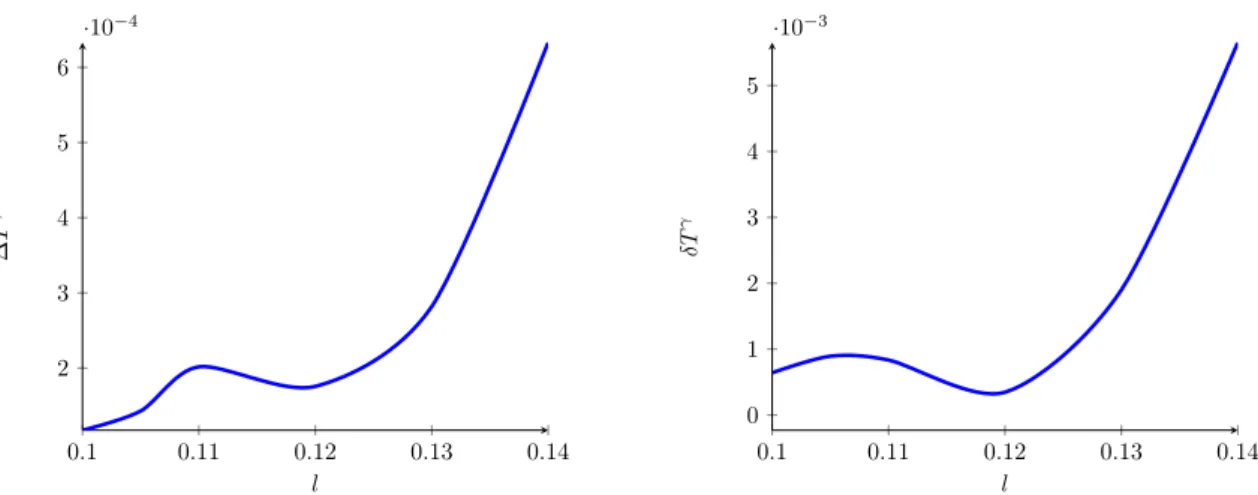
(l) defined in (3.57) is shown.

where ¯ T ^γ is the average over all considered configurations M ∈ { m 1 , . . . , m 2 } and l ∈ [1, 1.05, . . . , 1.4], m ₁ was chosen to be 10, m ₂ was chosen to be 23, k was kept fixed at k = 0.99. The maximal relative difference between two results for the coupling corrected temperature corresponding to the various choices for M and l is

δT ^max := T max ^γ − T _min ^γ

T ¯ ^γ = 0.00565, (3.56)

where both the minimal and the maximal value for T ^γ appear in the case l = 0.14, the maximal l-value of our analysis. Finally let us consider the function

δT (l) := T max ^γ (l) − T _min ^γ (l)

T ¯ ^γ , (3.57)

where T _max/min ^γ (l) is the maximal/minimal value for T ^γ we obtained for a certain l. The

results are displayed in figure 2.

JHEP08(2019)006

10 11 12 13 14 15 16 17

294.7 294.8 294.9 295 295.1 295.2

M

T

Figure 3. The higher derivative correction T

for to the temperature, computed on intervals [0.1, k] for different values of M (shown in a smoothed plot). The solid blue line shows the results for k = 0.975, the dashed red line corresponds k = 0.98, the dotted black line corresponds to k = 0.985 and the solid green line corresponds to k = 0.99. The metric was extrapolated to u = 1.

In figure 3 we display the results for the correction factor to the temperature obtained by calculations on intervals [0.1, k], we extrapolated the resulting coupling corrections to the metric to u = 1.

3.4 Approximating higher derivative corrections to tensor QNMs without magnetic background field

Let us now turn to fluctuations of the metric of a coupling corrected AdS-Schwarzschild black hole. Quasinormal modes are tiny perturbations of the geometry, which can be sepa- rated according to their transformation behaviour, respectively with the help of symmetry arguments. They are dual to quasiparticles on the field theory side and encode the re- sponse of the system to excitations around the equilibrium. We will consider tensor, or spin-2-fluctuations h x,y in the x, y-plane with momentum in z direction. In this section we are going to approximate higher derivative corrections to these tensor QNMs without considering background magnetic fields. The coupling corrections to spin-2-QNMs in this setup were first computed in [17]. Our aim is to reproduce these results by applying a technique, which can be extended to derive coupling corrections to tensor QNMs of the coupling corrected magnetic black brane geometry, which we now know on an interval [l, k] ⊂ [0, 1]. We consider the linearized differential equations obtained by varying the higher derivative corrected action with respect to fluctuations h _xy dxdy of the background geometry. These EoM were first derived in [7] and are given in the appendix (A.1). The characteristic exponents of the differential equation (A.1) are given by ± ^iˆ ₂ ^ω , such that

h = (1 − u) ⁻

φ(u) (3.58)

where φ(u) is regular at the horizon and the exponent of (1 − u) ⁻

was chosen to corre-

spond to infalling wave solutions. Here ˆ ω is defined as ˆ ω = _2πT ^ω to be consistent with the

JHEP08(2019)006

convention in [17]. In the case of b = ⁵ ₄ we will use the convention ˆ ω = _πT ^ω , ˜ ω = _r ^ω

h

to be consistent with [2]. Considering the grid (3.33) again, we define the discrete differentiation matrix A(M ) as

A(M) _ij = 2

k − l ∂ _u c _{j u→u}

i

, (3.59)

where c _j is the j-th Chebyshev cardinal function corresponding to the j-th grid point 2u _j

k − l + l + k

l − k . (3.60)

An equivalent and numerically more convenient definition of A(M ) is given in [27]. Ex- panding φ in Chebyshev cardinal functions ˜ c corresponding to the grid (3.33) in the form

φ(u) =

M

X

i=0

˜

c i (u)a i (3.61)

allows us to formulate (A.2) as a matrix equation for the zero momentum mode q = 0

O(M, γ, ω)v ˆ = 0 (3.62)

with v = (a _i ) i∈{0,...,M} and O(M, γ, ω) ˆ ji =

M

X

l=0

f 2 (u j )A(M ) jl A(M ) li + f 1 (u j , γ, ω)A(M ˆ ) ji + f 0 (u j , γ, ω)δ ˆ ji , (3.63) the function f _i for q = 0 are given in the appendix A. We can split up O(M, γ, ω) as ˆ

O(M, γ, ω) = ˆ O ⁰ (M, γ ) + ˆ ωO ¹ (M, γ ) + ˆ ω ² O ² (M, γ ). (3.64) This allows us to write (3.62) as a generalized Eigenvalue problem

O ⁰ (M, γ ) O ¹ (M, γ)

0 1

! v ˆ ωv

!

= ˆ ω 0 − O ² (M, γ)

1 0

! v ˆ ωv

!

. (3.65)

The idea is to solve (3.65) for ˆ ω exactly in γ with γ = ζ (3)

8 1000 ^−3/2 1 − cos( ^πn _˜

M )

2 . (3.66)

We chose n ∈ { 0, . . . , M ˜ } , ˜ M = 80. This Gauss-Lobatto grid corresponds to λ values between λ = ∞ and λ = 1000. The slopes at λ = ∞ of the curves of partially resummed coupling corrected results for ˆ ω in the complex plane will give us the O (γ ¹ )-corrections to the QNM frequency ˆ ω. The boundaries of the interval on which the Gauss-Lobatto grid (3.33) lives are chosen to be l = 0.1 and k = 0.99. We depict the coupling corrections to the first QNM in figure 4. The results are displayed for different values of the grid size M and show clear convergence towards the exact coupling corrections obtained in [17]. We plotted the first order coefficients of the γ-expansion of the first QNM frequency.

ˆ

ω ¹ := ∂ _γ ω ˆ | γ=0 . (3.67)

JHEP08(2019)006

6 8 10 12 14

1,100 1,150 1,200 1,250 1,300

M Im( ˆω

)

6 8 10 12 14

1,500 1,550 1,600 1,650 1,700 1,750

M Re( ˆω

)

Figure 4 . The first order correction ˆ ω

to the lowest tensor-QNM frequency for b = 0, q = 0, computed via spectral methods on a grid u ∈ [0.1, 0.99] (solid blue line) compared with the exact result (red dashed line) for different values of M shown in a smoothed plot.

Applying this method with 25 M corrupts the results noticeably. For 10 < M <

20 we obtain good agreement with the already known results. Since the aim is to give a numerical approximation to the higher derivative corrections of tensor QNMs in the presence of a strong magnetic background field, that backreacts on the coupling corrected geometry, we take this result as motivation to apply this technique in the case b = ⁵ ₄ .

3.5 Approximating higher derivative corrections to the first tensor QNM in the presence of a strong magnetic background field

The way we have chosen our background field together with considering fluctuations ensures that the linearized differential equations for h _x,y decouple from those of other fluctuations.

Our aim is to determine γ -corrections to the results in [2]. As before the calculation is done for the case q = 0. We already have found the metric, respectively the functions U , U, V, W, L ˜ up to order O (γ ) for the parameter b = ⁵ ₄ in the previous sections. The following metric ansatz describes tensor fluctuations of this geometry

ds ² _fluc = − U (u)dt ² + ˜ U (u)du ² + e ^{2V (u)} (dx ² + dy ² ) + e ^{2W (u)} dz ² + L(u) ² 4b ² x ² 3 dy ² + L(u) ² 2bx

√ 3 dy dy 3 sin(y 1 ) ² + dy 4 cos(y 1 ) ² sin(y 2 ) ² + dy 5 cos(y 1 ) ² cos(y 2 ) ²

× L(u) ² dy ² ₁ + cos(y 1 ) ² dy ² ₂ + sin(y 1 ) ² dy ₃ ² + cos(y 1 ) ² sin(y 2 ) ² dy 4 + cos(y 1 ) ²

× cos(y 2 ) ² dy ² ₅

+ h x,y (u, t)dxdy. (3.68)