JHEP07(2018)069
Published for SISSA by Springer
Received: June 25, 2018 Accepted: June 26, 2018 Published: July 10, 2018
Studying a charged quark gluon plasma via holography and higher derivative corrections
Sebastian Waeber and Andreas Sch¨ afer
Department for Theoretical Physics, University of Regensburg, Universit¨atsstrasse 31, 93040 Regensburg, Germany
E-mail: sebastian.waeber@physik.uni-regensburg.de, andreas.schaefer@physik.uni-regensburg.de
Abstract: We compute finite ’t Hooft coupling corrections to observables related to charged quantities in a strongly coupled N = 4 supersymmetric Yang-Mills plasma. The coupling corrected equations of motion of gauge fields are explicitly derived and differ from findings of previous works, which contained several small errors with large impact. As a consequence the O (γ)-corrections to the observables considered, including the conductivity, quasinormal mode frequencies, in and off equilibrium spectral density and photoemission rates, become much smaller. This suggests that infinite coupling results obtained within AdS/CFT are little modified for the real QCD coupling strength.
Keywords: AdS-CFT Correspondence, Holography and quark-gluon plasmas
ArXiv ePrint: 1804.01912
JHEP07(2018)069
Contents
1 Introduction 1
2 Einstein-Maxwell-AdS/CFT in the λ → ∞ limit 2
3 Finite coupling corrections to the EoMs of gauge fields 7
4 Results 20
4.1 Quasinormal modes and their coupling corrections 20
4.2 Finite coupling corrections to the plasma conductivity and photoemission rate 22 4.3 Finite coupling corrections to the off-equilibrium spectral density 24
4.4 A partial resummation of the expansion in γ 28
5 A surprising observation 29
6 Discussion 33
A Variation of the higher derivative terms with respect to the five form 35
1 Introduction
Experimental data from heavy ion collisions at LHC and RHIC suggest that the produced quark gluon plasma (QGP) is strongly coupled and equilibrates extremely fast. Unfor- tunately, standard QCD techniques are unsuitable to treat the strongly coupled, non- equilibrium early dynamics. Therefore the best known way to study the early phases of the QGP before thermalization happened is via holography, by mapping weakly coupled supergravity (SUGRA) to its strongly coupled quantum field theoretical dual. Although there is no dual description for QCD one can approach the real world by studying the plasma with the help of the holographic dual of large-N , N = 4 strongly coupled super Yang-Mills (SYM) theory.
The QGP produced during heavy ion collisions lies somewhere in between the two extreme limits of infinitely strong coupling (or small curvature) with ’t Hooft coupling λ = ∞ and weak coupling, which would allow for a perturbative description. One way of investigating this region is to consider finite coupling corrections or higher derivative corrections to the type IIb SUGRA action. These additional contributions of order O (α
03) for the dual gravity theory, where α
0is related to the string length l
svia α
0= l
2s, yield finite coupling corrected correlators, emission rates, transport coefficients etc. on the QFT side.
One interesting topic in this context is the analysis of the behaviour of charged parti-
cles in such a QGP. In recent years there have been several works contributing to a deeper
quantitative understanding thereof. One important step was the computation of leading
JHEP07(2018)069
coupling corrections to the equations of motion of gauge fields in a strongly-coupled N = 4 SYM plasma by considering O (α
03) corrections to the type IIB supergravity action [1, 2].
These α
0-corrected equations of motion were then used to study the conductivity, the trans- port coefficient in this channel and the photoemmission rate, which give important infor- mation about the structure of the plasma. Determining α
0corrections to these quantities is of major interest, especially since this allows first cautious comparisons and interpolations between the spectra of strongly coupled and weakly coupled plasmas [2]. Unfortunately the authors of [1, 2] used a 5-form that didn’t solve its higher derivative corrected EoM. In addition, unlike stated in these papers, the calculation was done in Euclidean signature, but the five form wasn’t transformed appropriately. More specifically, we can reproduce their results, if we leave out an actually needed factor i in front of the five form components of the form dt ∧ . . . after the transformation to Euclidean signature. Also several terms contributing to the Hodge duals got lost. Our first aim is to give a corrected derivation of the higher derivative corrected EoM for gauge fields in type IIb SUGRA. After that we revisit the computation of several observables, whose α
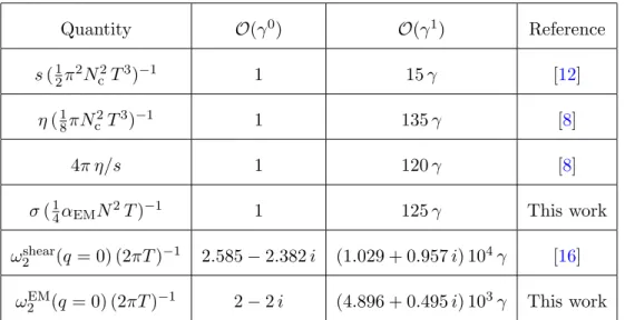
03-corrections so far have been calculated with the EoM form [1, 2]. In general we find that the actual higher derivative corrections to all quantities studied in this paper turn out to be substantially smaller than the values found in the literature so far. For instance in [1] the correction factor to the conductivity was given as (1 +
149939γ ), whereas we obtained (1 + 125γ ). A comparison with the transport coefficient of the spin 2 channel is given in table 2.
In contrast to previous works we find that the behaviour of the photoemission rate and spectral density at finite coupling agree with expectations from weak coupling calculations in both the small and, that is new, the large energy limit [7]. In [7] the authors derived that in the weak coupling limit decreasing coupling means increasing phtotoemission rate at small momenta and decreasing photoemission rate at large momenta. The signs of the correction factors we found coincide with these expectations. We start from the higher derivative corrected type IIb action and compute finite coupling corrected QNM spectra, spectral density, photoemission rate and conductivity of the plasma. Before we come to finite coupling corrections we give a detailed description how to introduce gauge fields in type IIb SUGRA by twisting the five sphere along certain angles, which was first described in [10]. We try to provide enough details of the calculations to allow the reader to check it with limited effort.
2 Einstein-Maxwell-AdS/CFT in the λ → ∞ limit
The aim of this section is to give a detailed description of how to introduce charge and gauge fields in AdS/CFT starting from the type IIb SUGRA action
S
10= 1 2κ
10Z
d
10x p
− det(g
10)
R
10− ∂
µφ∂
µφ − 1 4 × 5! F
52, (2.1)
where F
5is the 5-form and g
10the metric of the 10 dimensional manifold. In the following
calculations we set the constant l, which measures the size of S
5, to 1, since the resulting
EoM for gauge fields won’t depend on it. In [10] it was shown that in order to obtain
JHEP07(2018)069
Maxwell-terms F
µνF
µνin the reduced 5 − dimensional theory one has to twist the five sphere S
5along its fibers in a maximally symmetric manner. The ansatz for the metric in this case has the form
ds
210= ds
2AdS+
3
X
i=1
dµ
2i+ µ
2idφ
i+ 2
√ 3 A
µdx
µ 2, (2.2)
with
ds
2AdS= − r
2h1 − u
2u dt
2+ 1
4u
2(1 − u
2) du
2+ r
h2u (dx
2+ dy
2+ dz
2), (2.3) where the unperturbed metric is just the AdS Schwarzschild black hole solution times S
5with horizon radius r
h. It is convenient to work here with the following S
5-coordinates, for which we define µ
iwith i ∈ { 1, 2, 3 } to be the direction cosines
µ
1= sin(y
1), µ
2= sin(y
2) cos(y
1), µ
3= cos(y
1) cos(y
2), (2.4) and set the angles
φ
1= y
3, φ
2= y
4, φ
3= y
5, (2.5) such that the metric of the 5 − sphere is given as
dΩ
25=
3
X
i=1
dµ
2i+ µ
2idφ
2i= dy
21+ cos(y
1)
2dy
22+ sin(y
1)
2dy
23+
+ cos(y
1)
2sin(y
2)
2dy
24+ cos(y
1)
2cos(y
2)
2dy
52. (2.6) It is straightforward to check that with this metric ansatz we obtain
R
10= R
A10µ→0− 1
3 F
µνF
µν, (2.7)
with F = dA. The dilaton part of the action can be ignored here, since its EoM does not couple with those of A
µand the solution of its EoM in this order in α
0is simply zero. On the other hand it is crucial to understand in detail the role of the five form part of the action in this calculation. In the following we will motivate its ansatz, which was given in [10].
The five form F
5is not an independent field with respect to which we have to vary the action in order to complete the set of EoM for type IIb fields relevant in this case.
Actually, the term F
52in the action is the kinetic term of the 4-form C
4with dC
4= F
5, which straightforwardly leads to the EoM obtained by varying S
10with respect to C
4:
d ∗ F
5= 0, (2.8)
where ∗ is the Hodge star operator. In addition one has dF
5= 0, which already reveals the self dual structure of the solution for F
5in this order in α
0.
In the case of a vanishing gauge field A
µ= 0 the self dual solution to (2.8) is F
5el= − 4
AdS= − 4 √
− g
AdSdt ∧ du ∧ dx ∧ dy ∧ dz, (2.9)
F
5= (1 + ∗ )F
5el, (2.10)
JHEP07(2018)069
where
AdSis the volume form of the AdS-part of the manifold. The forefactor − 4 is chosen in such a way that in the dimensionally reduced action we have
vol(S
5) 2κ
10Z
d
5x p
− det(g
AdS)
R
5− 8 + R
S5= vol(S
5) 2κ
10Z
d
5x p
− det(g
AdS)
R
5+ 12
. (2.11) Now we want to find a solution for dF
5= 0 and d ∗ F
5= 0 with the metric (2.2). In order to see that F
5el= −
4lAdSis no longer the correct ansatz we consider the tuyzy
1y
3-direction of the 6-form d ∗ F
5. In the following we only consider transverse fields, which means that only A
xis non-vanishing and A
x= A
x(u, t, z). The deduction for longitudinal fields is analogous. Remember that we are interested in linearized differential equations for A
µ, which we consider as tiny fluctuations of our background geometry. This means that terms of order A
2µor higher can be discarded, such that there are only 6 non-diagonal elements in the matrix representation of the metric tensor g
µν, namely g
xy3, g
xy4, g
xy5and interchanges of x and y
i. From our solution in the A
µ= 0 case we already know that we will at least have one non vanishing term in the tuyzy
3-direction of the 5-form ∗ F
5, which is proportional to
√ − gg
y1y1g
y2y2g
y3xg
y4y4g
y5y5(F
5Aµ→0)
y1y2y3y4y5. (2.12) Note that we are not making use of the sum-convention here and henceforth. This term is proportional to A
µwithout any derivatives and has a non trivial y
1-dependence, such that we have
0 6 = (d ∗ F
5)
tuyzy1y3= ∂
y1( √
− gg
y1y1g
y2y2g
y3xg
y4y4g
y5y5(F
5Aµ→0)
y1y2y3y4y5) + . . . (2.13) without further directions of F
5being non zero. This term can’t be canceled by the EoM for A
µ, since it would give a mass to our gauge field. Consequently there have to be more components of the solution for F
5, which give non-zero contributions, such that these mass terms cancel. The symmetries of this problem should dictate, which directions of the five form vanish and which don’t. We instead use a different approach. We start from the fact, that our final ansatz for the C
4can only depend on the coordinates u, t, z, y
1, y
2, i.e. the coordinates the metric and its fluctuations A
µdepend on. Any other dependence would lead to non-vanishing components of d ∗ dC
4. This means the only possible components of C
4proportional to A
µthat could give a contribution to the tuyzy
1y
3-component of d ∗ dC
4are (C
4)
xy1y4y5, (C
4)
xy2y4y5, (C
4)
xzy4y5, (C
4)
txy4y5, (C
4)
uxy4y5modulo permutations of their 4 indices. In the following, when we address properties of certain directions of forms, e.g.
for (C
4)
abcdthe abcd-direction of C
4, these properties’ applicabilities implicitly include all permutations of the indices abcd with the correct signs.
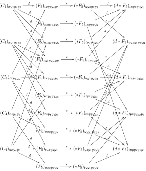
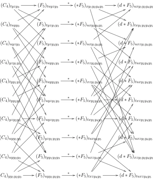
Graphically we can depict all relevant contributions of these 4-form components to the
differential equations shortly written as d ∗ dC
4= 0 as shown in figure 1. Note that this
diagram is closed in the sense that plus the contribution in (2.13) all terms contributing
to the tuyzy
1y
3, uyzy
1y
2y
3, tuyzy
2y
3, tyzy
1y
2y
3and tuyy
1y
2y
3-directions of d ∗ F
5are
depicted and (C
4)
xy1y4y5, (C
4)
xy2y4y5, (C
4)
xzy4y5, (C
4)
txy4y5, (C
4)
uxy4y5do not contribute
to any other directions of d ∗ F
5. The next important observation is that (d ∗ F
5)
uyzy1y2y3,
(d ∗ F
5)
tyzy1y2y3and (d ∗ F
5)
tuyy1y2y3cannot be set to 0 by imposing the EoM of A
x, because
JHEP07(2018)069
(C
4)
xy2y4y5 d //d
''d
d
(F
5)
txy2y4y5 ∗ //( ∗ F
5)
uyzy1y3 d //d
""
(d ∗ F
5)
tuyzy1y3(F
5)
xzy2y4y5 ∗ //( ∗ F
5)
tuyy1y3d 66
d
(C
4)
xy1y4y5d
''d
d
d
(F
5)
uxy2y4y5 ∗ //( ∗ F
5)
tyzy1y3d
<<
d
(d ∗ F
5)
uyzy1y2y3(F
5)
xy1y2y4y5∗ //
( ∗ F
5)
tuyzy3d
BB
d
((
(C
4)
txy4y5d
GG
d //
d
d
(F
5)
txy1y4y5∗ //
( ∗ F
5)
uyzy2y3d //
d
<<
(d ∗ F
5)
tuyzy2y3(F
5)
uxy1y4y5∗ //
( ∗ F
5)
tyzy2y3d 66
d
((
(C
4)
xzy4y5d
HH
d //
d
''
d
(F
5)
xzy1y4y5∗ //
( ∗ F
5)
tuyy2y3d
<<
d
""
(d ∗ F
5)
tyzy1y2y3(F
5)
uxzy4y5∗ //
( ∗ F
5)
uyy1y2y3d
((
d
GG
(C
4)
uxy4y5d
''
d //
d
DDd
JJ
(F
5)
tuxy4y5 ∗ //( ∗ F
5)
yzy1y2y3d
<<
d
II
(d ∗ F
5)
tuyy1y2y3(F
5)
uxzy4y5 ∗ //( ∗ F
5)
tyy1y2y3.
d 66
d
BB
Figure 1. Graphic depiction of the “closed” system of differential equations around the xy2y4y5- direction ofC4. In this order inα0 the right hand side should give zero.
they contain odd derivatives in the t and z direction ∂
zA
x, ∂
tA
xor ∂
z3A
x, ∂
t3A
x, if we have only even derivatives in (d ∗ F
5)
tuyzy1y3.
From the requirement that there are no mass terms in the EoM for A
xwe can deduce
from (2.13) and the form of F
5Aµ→0that ( ∗ F
5)
tuyzy3is proportional to sin(y
1)
2and has no
y
2-dependence. Therefore, (C
4)
xy1y4y5doesn’t contribute to (d ∗ F
5)
tuyzy1y3and (C
4)
xy2y4y5doesn’t contribute to (d ∗ F
5)
tuyzy2y3. Thus, it is legal to choose (C
4)
xy1y4y5= 0. This
leads to the beautiful result that in diagram 1 the contributions of (C
4)
xzy4y5, (C
4)
txy4y5,
(C
4)
uxy4y5to (d ∗ F
5)
tuyzy1y3have the same form as those of (C
4)
xy2y4y5and are indistin-
guishable in the final EoM (d ∗ F
5)
tuyzy2y3= 0 , which means it is a legitimate ansatz to
set them to 0 and solve (d ∗ F
5)
tuyzy2y3= 0 for (C
4)
xy2y4y5. This process has to be repeated
for two further cases (remember that we only considered the off diagonal element g
xy3so
JHEP07(2018)069
far), which together with the self duality of the 5-form leads to the result (F
50)
el= − 4
AdS, (F
51)
el= 1
√ 3
3
X
i=1
d(µ
2i) ∧ dφ
i∧ ¯ ∗ F
2, (2.14) and
F
5= (1 + ∗ )((F
50)
el+ (F
51)
el), (2.15) with F
2= dA. Of course, it isn’t a coincidence that the electric part of F
5is proportional to J ∧ ¯ ∗ dA, with the K¨ ahler-form of the five sphere J , and there are more and easier ways to deduce this five form solution. Since we will have little choice but to work with similar brute force in the O (α
03)-case, due to the complexity of the higher derivative correction terms to the type IIb action, it is a good exercise to already do this in the lowest order in α
0. Notice that the requirement that we are allowed to make the ansatz (2.2) implies that the EoM for A
µcan be obtained both by varying the action with respect to A
µand from the tuyzy
1y
3, tuyzy
2y
4,tuyzy
2y
5,tuyzy
1y
5and tuyzy
1y
4-directions of d ∗ dC
4= 0, simply by starting from the fact that the metric tensor g
µνhas only certain off-diagonal elements.
Varying the action with respect to A
µleads to the following well known EoM for transverse fields in order O (γ
0)
∂
u2A
x− 2u
1 − u
2∂
uA
x+ ω ˆ
2− q ˆ
2(1 − u
2)
u(1 − u
2)
2A
x= 0 (2.16) with ˆ x =
2rxh
=
2πTxfor x ∈ { q, ω } and the horizon radius r
h. Before we address higher derivative corrections it is advisable to look in detail at the following calculational pre- scription of SUGRA to obtain an effective action solely for the metric: “Take the ansatz of the 5 − form, plug it back into the action and only consider the magnetic part of your F
5and double its contribution, then vary with respect to the metric.”. In order to be able to decide, whether we are allowed to make use of this, if we include higher derivative correc- tions, we must understand where this prescription comes from. In the easiest case, where we do not consider α
0-corrections or gauge fields A
µ, our solution for the five form is given in (2.9), (2.10). If we want to derive the EoM for general metric components from the type IIb action (3.2) we, of course, are not allowed to impose a dependence of the five form on g
µνon the level of the action. Instead we have to vary the five form part of the action as follows
δ Z
d
10x √
− g
− 1 4 · 5! F
52= − 1 4 δ
Z
d
10x √
− g
g
ttg
uug
xxg
yyg
zz(F
5el)
2tuxyz+ + g
y1y1g
y2y2g
y3y3g
y4y4g
y5y5(F
5mag)
2y1y2y3y4y5= − 1 4 δ
Z d
10x
−
r g
y1y1g
y2y2g
y3y3g
y4y4g
y5y5g
ttg
uug
xxg
yyg
zz× (F
5el)
2tuxyz+
r g
ttg
uug
xxg
yyg
zzg
y1y1g
y2y2g
y3y3g
y4y4g
y5y5(F
5mag)
2y1y2y3y4y5, (2.17)
which leads to a contribution to the EoM for g
µνof the form 4
( − 1)
1+P5i=1δµyi√ − g
2 g
µν− ( − 1)
P5i=1δµyi√ − g 2 g
µν. (2.18)
JHEP07(2018)069
The same result is obtained from plugging the solution of the five form back into the action, only considering the contribution of the magnetic part times 2. This calculation can be performed similarly for more complicated five form solutions involving gauge fields. This recipe, which is nothing but a calculational tool, is equivalent to the more intuitive but also more tedious approach of treating every metric component and every 4-form component as an independent field on the level of the action, varying with respect to all of them and solv- ing the resulting system of EoM. One important lesson to learn here is that the justification for this prescription requires a self dual five form and we will see in the next section, that self duality is violated when we include higher derivative corrections (also see [5]). We don’t want to imply that this prescription breaks down for all non self dual forms, but we are not aware of a justification to use it to deduce the EoM for higher orders in α
0. Out of caution we will avoid this simplification in order O (α
03) and strictly following the variational principle.
3 Finite coupling corrections to the EoMs of gauge fields
Now let us start to consider higher derivative corrections to our theory. In type IIb SUGRA this means that we have to add terms of order α
03to the action (3.2). For this purpose we set γ =
ζ(3)8λ
−32, with the ’t Hooft coupling λ, which is proportional to α
0−12. The action including finite λ corrections has the form
S = S
10+ γS
10γ+ O (γ
43), (3.1) with
S
10= 1 2κ
10Z
d
10x √
− g
R
10− 1 4 × 5! F
52. (3.2)
as before and
S
γ10= 1 2κ
10Z
d
10x p
| g
10|
C
4+ C
3T + C
2T
2+ C T
3+ T
4. (3.3)
The expression for S
10γis schematical and stands for a set of tensor contractions between the Weyl tensor C and T , a 6-tensor that takes care of higher derivative corrections containing the five form. Explicitly the term in brackets in (3.3) is given by [5]
γW = γ
C
4+ C
3T + C
2T
2+ C T
3+ T
4= γ
86016
20
X
i=1
n
iM
i, (3.4)
with
(n
i)
i=1,...,20= ( − 43008, 86016, 129024, 30240, 7392, − 4032, − 4032, − 118272,
− 26880, 112896, − 96768, 1344, − 12096, − 48384, 24192, 2386,
− 3669, − 1296, 10368, 2688) (3.5)
JHEP07(2018)069
as well as
(M
i)
i=1,...,20= (C
abcdC
abefC
ceghC
dgfh, C
abcdC
aecfC
bgehC
dgfh, C
abcdC
aefg
C
bf hiT
cdeghi, C
abcdC
abceT
df ghijT
ef hgij, C
abcdC
abefT
cdghijT
ef ghij, C
abcd
C
aecfT
beghijT
df ghijC
abcdC
aecfT
bghdijT
eghf ij, C
abcd
C
aef gT
bcehijT
df hgij, C
abcdC
aef gT
bcehijT
dhif gj, C
abcdC
aefgT
bcf hijT
dehgij, C
abcdC
aef gT
bcheijT
df hgij, C
abcdT
abef ghT
cdeijkT
f ghijk, C
abcdT
abef ghT
cdf ijkT
eghijk, C
abcdT
abef ghT
cdf ijkT
egih jk, C
abcdT
abef ghT
cef ijkT
dghijk
, T
abcdefT
abcdghT
egijklT
f ijhkl, T
abcdefT
abcghiT
dejgklT
fhkijl
, T
abcdefT
abcghiT
dgjeklT
fhj iklT
abcdefT
abcghiT
dgjeklT
fhkijl
, T
abcdefT
aghdijT
bgkeil
T
chkfjl
). (3.6) The Weyl tensor C
abcdis
C
abcd= R
abcd− 1
8 g
acR
db− g
adR
cb− g
bcR
da+ g
bdR
ca+ 1
72 Rg
acg
db− Rg
adg
cb, (3.7) and T is given by
T
abcdef= i ∇
aF
bcdef++ 1
16 F
abcmn+F
def+mn− 3F
abf mn+F
dec+mn, (3.8)
with two sets of antisymmetrized indices a, b, c and d, e, f . In addition the right hand side of (3.8) is symmetrized with respect to the interchange of (a, b, c) ↔ (d, e, f ) [5]. Here F
+stands for the self dual part
12(1 + ∗ )F
5of the five form. It should be noted that up to this day it is not known, whether the terms in (3.3), which were derived in [5] using [19], are complete. There are strong indications that this is the case, but since there is no strict mathematical proof we included this cautionary remark.
We already know that the solution of F
5in order O (γ
0) is self dual, and that in order O (γ
1) the O (γ
0) part of F
5is the only contribution of F
5that enters in the higher derivative part of the action. But we still do not have the EoMs in order O (γ) for the 4-form compo- nents. This means that we still have to vary the action with respect to C
4and thus it makes a difference whether F
5= dC
4or F
+enters γW . Before we start discussing the higher derivative corrected EoMs for gauge fields, we have to determine the γ -corrected solution of our unperturbed geometry as done in [4]. The ansatz for the metric we make is of the form ds
210= − r
h2U (u)dt
2+ ˜ U (u)du
2+ e
2V(u)r
h2(dx
2+ dy
2+ dz
2) + L(u)
2dΩ
25, (3.9) where we are forced to give up the product structure of our manifold and admit a u- dependent warping factor L(u) in front of the 5-sphere line element as shown in [4]. The EoMs for our 4-form components still have the form (2.8) simply because the T -tensor defined above vanishes on the unperturbed background. We also have
δS
10γδF
5= 0 (3.10)
JHEP07(2018)069
for A
µ= 0. The solution for the 5-form in order O (γ
1) and without gauge fields is
F
5= (1 + ∗ )F
5el(3.11)
F
5el= − 4
L(u)
5γAdS, (3.12)
where
γAdSis the volume form of the γ -corrected AdS-part of our manifold. The five form is still self dual, such that we are allowed to plug the solution for the five form back into the action, only considering its magnetic part and doubling its contribution, which gives
1 2κ
10Z
d
10x p
− det(g
10)
R
10− 8
L(u)
10+ γW
. (3.13)
The EoM for the metric components from this action yield [4]
U (u) = (1 − u
2) u
1 + 5u
2γ
8 ( − 130 − 130u
2+ 67u
4)
(3.14) U ˜ (u) = 1
4u
2(1 − u
2)
1 + γ 325
4 u
2+ 1075
16 u
4− 4835 16 u
6(3.15) V (u) = − 1
2 log(u) (3.16)
L(u) = 1 + 15γ
32 (1 + u
2)u
4. (3.17)
Now we are ready to introduce gauge fields to our finite λ-corrected theory. In order to get the correct results in the limits A
µ→ 0 and γ → 0 we choose the ansatz again corresponding to a twist of the five sphere along the y
3, y
4, y
5angles
ds
210= − r
2hU (u)dt
2+ ˜ U (u)du
2+ e
2V(u)r
2h(dx
2+ dy
2+ dz
2) + L(u)
24A
x(u, t, z)
23 dx
2+ L(u)
24A
x(u, t, z)
√ 3 dx dy
3sin(y
1)
2+ dy
4cos(y
1)
2sin(y
2)
2+ dy
5cos(y
1)
2× cos(y
2)
2+ L(u)
2dy
21+ cos(y
1)
2dy
22+ sin(y
1)
2dy
32+ cos(y
1)
2sin(y
2)
2dy
4+ cos(y
1)
2cos(y
2)
2dy
52, (3.18)
which we justify as follows: we will obtain the EoM for A
µby varying the coupling cor- rected type IIb SUGRA action with respect to the 4-form components and A
µ. Apparently the xx-component e
2V(u)+ L(u)
2 4Ax(u,t,z)3 2of our metric ansatz looks like it could lead to problems. On the one hand we know that if we would only vary the action with respect to e.g. the xy
3-component, we would obtain an EoM for A
µthat is at first glance different from varying the action with respect to A
µ. This is because after linearizing in A
µthe A
2µ- term of the xx-component of the metric won’t contribute to the former case, but will give a contribution to the latter. In fact varying the √
− gR
10, √
− g
4∗5!1F
52and √
− gγW -terms
in the action with respect to the xy
3-component of the metric separately and inserting the
ansatz (3.18) gives mass terms. However, adding everything up leads to the same EoM for
A
µ(of course, still depending on some unknown F
5-directions) as varying with respect to
A
µ, while the mass terms cancel identically.
JHEP07(2018)069
From now on we will work with r
h= 1, which also applies for the appendix A, and reintroduce r
hwherever needed after having obtained the EoM or contributions thereto.
We know that we will end up with differential equations, where r
honly appears in the rescaled frequency
2rωh
and momentum
2rqh
. Also setting r
h= 1 simply corresponds to rescaling t the spatial coordinates and A
xby a constant factor. Changing
ω2to
2rωh
in the end corresponds to scaling back to the form of the metric given in (3.18).
Now we are prepared to determine the EoM in order O (γ ) of all relevant fields i.e.
gauge fields, the five-form and, less important, the dilaton field. Since its EoM decouple, we will ignore it henceforth. Let us start with the five-form. As in the last section its EoMs are derived by varying the action with respect to the 4-form components with dC
4= F
5. A concise way of writing the resulting system of differential equations is
d
∗ F
5− ∗ 2γ
√ − g δ W δF
5= 0, (3.19)
where
δWδF5
is defined by
δ W
δF
5:= 2κ
10δS
10γδF
5. (3.20)
It is easy to obtain this by observing that for a p-form C with F = dC and an action S =
Z
d
DxL(F, ∇ F ) (3.21)
for C the variation
δCδS= 0 leads to an equivalent set of differential equations as d
∗ 1
√ − g δS δF
= 0. (3.22)
The first and easiest result we can extract from (3.19) is that self duality of the five form is broken if d ∗
√1−gδWδF56 = 0, which is the case if A
µ6 = 0. Obviously, if F
5would still be self dual, we had (1 − ∗ )F
5= 0, but together with dF
5= 0 (3.19) would then lead to a contradiction. This means that we cannot treat the F
52-term of the action as in the previous cases. In the following let us focus on the variation of this term with respect to A
µ.
Due to the same argument as in the first section, since we are only interested in those terms of the final EoM, which are linear in A
µ, we can ignore O (A
2µ) parts of the metric in F
52. Contributions of terms of this form cancel identically, as they have to, since otherwise we would get mass terms. This means that the number of F
5-directions, which actually contribute to
δ √
− gF
52δA
µ(3.23) is very restricted. As in section one, we only consider transverse fields A
x(u, t, z), with A
y= A
z= 0. This implies that the only metric components depending on A
µ, modulo terms of order O (A
2µ), are again g
xy3, g
xy4, g
xy5, g
y3x, g
y4x, g
y5x. Therefore, the only directions of F
5, which contribute to (3.23) in order O (γ
1), are
(F
5)
y1y2y3y4y5, (F
5)
tuxyz, (F
5)
tuyzy3, (F
5)
tuyzy4, (F
5)
tuyzy5, (F
5)
xy1y2y4y5, (F
5)
xy1y2y3y5,
(F
5)
xy1y2y3y4. (3.24)
JHEP07(2018)069
We already know how (F
5)
y1y2y3y4y5and (F
5)
tuxyzlook like in order O (γ
1) for A
µ= 0 and how these directions are modified in order O (γ
0) for A
µ6 = 0. This is all the informa- tion we need about them, when computing (3.23), since (F
5)
tuyzy3, (F
5)
tuyzy4, (F
5)
tuyzy5, (F
5)
xy1y2y4y5, (F
5)
xy1y2y3y5, (F
5)
xy1y2y3y4are zero for A
µ= 0. This means we only have to compute (F
5)
tuyzy3, (F
5)
tuyzy4, (F
5)
tuyzy5, (F
5)
xy1y2y4y5, (F
5)
xy1y2y3y5, (F
5)
xy1y2y3y4up to first order in γ from (3.19). We will return to this later, let us first finish the variation of the rest of the action with respect to the gauge fields.
With our metric (3.18) we obtain R
10=
R
10 Aµ→0− L(u)
23 F
µνF
µν(3.25)
for the Ricci scalar. Varying this part with respect to A
µis straightforward. The final part δγ √
− g W
δA
µ(3.26)
already contains a γ-factor. Therefore, only O (γ
0)-parts of the metric and F
5enter it in order O (γ
1). Knowing already the solutions for F
5with gauge fields in zeroth order in γ allows us to compute this term immediately. One has to be careful and remember that only the self dual part of F
5enters here. Of course, we know already, that after having solved all EoM, we have (1 − ∗ )F
5= 0 in order O (γ
0). But since on the action level the 4-form components and the gauge fields are independent fields, meaning that
δAδF5µ
![Table 1 . The first two QNM frequencies at q = 2πT (right) and q = 0 (left) normalized by 2πT and their O (γ)-corrections, which turn out to be more than one order of magnitude smaller then found in [9], which was based on the EoM derived in [1–3].](https://thumb-eu.123doks.com/thumbv2/1library_info/3938814.1532891/23.892.136.758.123.223/table-frequencies-right-normalized-corrections-magnitude-smaller-derived.webp)
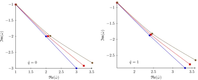
![Figure 5. The flow of the first 3 QNM frequencies, normalized by 2πT , with the ’t Hooft coupling between λ = ∞ and λ = 11.3 ≈ 4πα s N , with N = 3 and α s = 0.3 computed in the resummation scheme [11] with ˆq = 0 (left) and ˆq = 1 (right)](https://thumb-eu.123doks.com/thumbv2/1library_info/3938814.1532891/30.892.134.766.119.369/figure-frequencies-normalized-hooft-coupling-computed-resummation-scheme.webp)