Partial deconfinement at strong coupling on the lattice

JHEP02(2021)004

Published for SISSA by Springer

Received : June 15, 2020 Revised : October 5, 2020 Accepted : December 14, 2020 Published : February 1, 2021

Partial deconfinement at strong coupling on the lattice

Hiromasa Watanabe, ^a Georg Bergner, ^b Norbert Bodendorfer, ^c Shotaro Shiba Funai, ^d Masanori Hanada, ^e Enrico Rinaldi, ^f,g Andreas Schäfer ^c and Pavlos Vranas ^h,i

a

Graduate School of Pure and Applied Sciences, University of Tsukuba, Tsukuba, Ibaraki 305-8571, Japan

b

University of Jena, Institute for Theoretical Physics, Max-Wien-Platz 1, D-07743 Jena, Germany

c

University of Regensburg, Institute of Theoretical Physics, Universitätsstrasse 31, D-93053 Regensburg, Germany

d

Physics and Biology Unit, Okinawa Institute of Science and Technology (OIST), 1919-1 Tancha, Onna-son, Kunigami-gun, Okinawa 904-0495, Japan

e

Department of Mathematics, University of Surrey, Guildford, Surrey, GU2 7XH, U.K.

f

Arithmer Inc., R&D Headquarters, Minato, Tokyo 106-6040, Japan

g

RIKEN iTHEMS Program, Wako, Saitama 351-0198, Japan

h

Nuclear and Chemical Sciences Division, Lawrence Livermore National Laboratory, Livermore, CA 94550, U.S.A.

i

Nuclear Science Division, Lawrence Berkeley National Laboratory, Berkeley, CA 94720, U.S.A.

E-mail: watanabe@het.ph.tsukuba.ac.jp, georg.bergner@uni-jena.de, norbert.bodendorfer@physik.uni-r.de, shotaro.funai@oist.jp, m.hanada@surrey.ac.uk, erinaldi.work@gmail.com,

andreas.schaefer@physik.uni-regensburg.de, vranas2@llnl.gov

Abstract: We provide evidence for partial deconfinement — the deconfinement of a SU(M) subgroup of the SU(N ) gauge group — by using lattice Monte Carlo simulations.

We take matrix models as concrete examples. By appropriately fixing the gauge, we observe that the M ×M submatrices deconfine. This gives direct evidence for partial deconfinement at strong coupling. We discuss the applications to QCD and holography.

Keywords: Gauge-gravity correspondence, Lattice Quantum Field Theory, M(atrix) Theories

ArXiv ePrint: 2005.04103

JHEP02(2021)004

Contents

1 Introduction 1

2 Review of partial deconfinement 3

2.1 Motivation from gravity 5

2.2 Intuitive picture 6

2.3 BEC-confinement correspondence and meaning of Polyakov line 9

2.4 Remarks on negative specific heat 11

3 Partial deconfinement: the Gaussian matrix model 12

3.1 The Hamiltonian formalism 14

3.2 The path integral formalism and lattice Monte Carlo 15

3.2.1 Ensemble properties and master field 15

3.2.2 Distribution of X _I,ij 17

3.2.3 Correlation between scalars and gauge field 21 4 Partial deconfinement: the Yang-Mills matrix model 23 4.1 The properties of the ensemble and the master field on the lattice 25

4.1.1 Distribution of X _I,ij 26

4.1.2 Correlation between scalars and gauge field 26

4.2 Constrained simulation 28

4.2.1 Sanity checks 29

4.2.2 Distribution of X I,ij 29

4.2.3 Correlation between scalars and gauge field 31

4.2.4 Energy 32

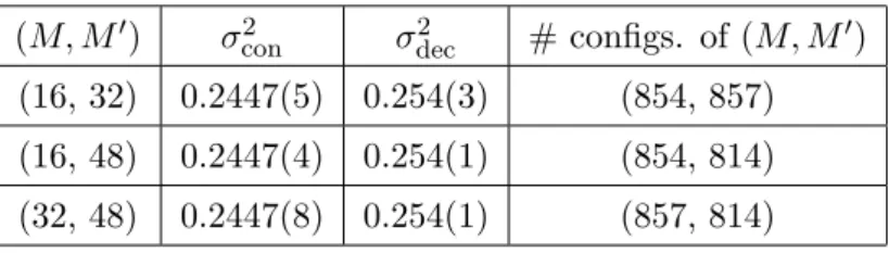
4.3 Summary of the numerical results 33

5 Conclusion and discussion 37

A Details of lattice simulation 40

A.1 Yang-Mills matrix model 40

A.1.1 A technical remark regarding the constrained simulation 40

A.2 Gaussian matrix model 41

B More on ρ ^(X) in Yang-Mills matrix model 41

JHEP02(2021)004

1 Introduction

Partial deconfinement [1–6] is the coexistence of confined and deconfined sectors in the space of colors (see figure 1: the partially deconfined phase lies between the completely confined phase (M = 0 in figure 1) and the completely deconfined phase (M = N in figure 1). A precise definition is given in section 2). Intuitively, the only difference from the common two-phase coexistence, say liquid and solid water at zero degree Celsius and one atmosphere, is that the separation is taking place in the internal space (the space of color degrees of freedom), rather than the usual space. As we will review in section 2, this difference leads to various interesting consequences, some of which are unexpected at first glance. In ref. [6] it was shown that partial deconfinement is analogous to superfluidity, in the sense that the confined and deconfined sectors resemble the superfluid and normal fluid. This rather unexpected analogy is explained in section 2.3, which makes it easier to grasp the physical mechanism of partial deconfinement.

So far, most of the studies of partial deconfinement have been limited to weakly coupled theories: there was no firm evidence beyond heuristic arguments that justified the existence of partial deconfinement at strong coupling. As a consequence, a sharp definition of partial deconfinement at strong coupling was missing. In this paper, we focus on a strongly- coupled theory and use numerical methods based on Lattice Monte Carlo simulations to investigate signals of partial deconfinement. Our results show that, at least for the model we study, the definition of partial deconfinement used at weak coupling can be adopted without change at strong coupling. In particular, the simplest order parameter is M itself, which is hidden in the theory in a nontrivial manner, as we will see in section 2.3. We show that the value of M determined in a few different manners coincide, which provides us with a strong consistency check. We will also discuss an explicit gauge fixing which makes the two-phase coexistence manifest.

As a concrete setup, we consider the gauged bosonic matrix model with SU(N ) gauge group. This theory’s action is the dimensional reduction of the (d + 1)-dimensional Yang- Mills action to (0 + 1)-dimensions. With the Euclidean signature that will be used in Lattice Monte Carlo simulations, the action is given by

S = N Z β

0

dt Tr 1

2 (D _t X _I ) ² − 1

4 [X _I , X _J ] ²

. (1.1)

Here I, J run through 1, 2, · · · , d (in this paper we focus on d = 9), β is the circumference

of the temporal circle which is related to temperature T by β = T ⁻¹ , and X _I ’s are N × N

hermitian matrices. The covariant derivative D t is defined by D t X I = ∂ t X I − i[A t , X I ],

where A _t is the gauge field. This model is often simply called “the Yang-Mills matrix

model”, or bosonic BFSS, because it is the bosonic part of the Banks-Fischler-Shenker-

Susskind matrix model [7, 8] when d = 9. The reasons to consider this model are its

simplicity and its close relation to the gauge/gravity duality. Moreover, this model has

been studied in the past, both in the weak coupling and the strong coupling regime, and

its phase structure at finite temperature is also known [9]. Building upon the current

literature on this model, we can focus on decisive signs of partial deconfinement.

JHEP02(2021)004

In the large-N limit, this model exhibits a confinement/deconfinement transition char- acterized by the increase of the entropy from O(N ⁰ ) to O(N ² ) [10]. Concerning this finite temperature transition, partial deconfinement is the phenomenon where only an SU(M ) subgroup of the SU(N ) gauge group deconfines, as pictorially shown in figure 1. To charac- terize partial deconfinement, it is convenient to define a continuous parameter identified by

M

N whose value can change from 0 to 1. Partial deconfinement happens between the com- pletely confined phase, with ^M _N = 0, and the completely deconfined phase, with ^M _N = 1.

These two phases have entropy and energy of order N ⁰ and N ² (up to the zero-point energy), respectively.

Now, suppose the energy is of order N ² , where is an order N ⁰ number and much smaller than 1. What kind of quantum states are dominant in the microcanonical ensemble at such intermediate energy range? The system cannot be in the confined phase because the energy is much larger than N ⁰ , but it cannot be in the deconfined phase either because the energy is much smaller than N ² . In partial deconfinement, where an SU(M ) subgroup deconfines, the energy and entropy are of order M ² , and hence by taking M ∼ √

N such intermediate values of the energy and entropy can be explained. Other explanations that may seem natural are discussed in section 2, together with the precise characterization of partial deconfinement.

The numerical study in ref. [9] appears to be consistent with the existence of this partially-deconfined phase. (See also refs. [11, 12] regarding the phase diagram, and refs. [13, 14] for pioneering numerical studies with limited numerical resources which clar- ified the qualitative nature of the transition.) In the d = 9 Yang-Mills matrix model, the partially-deconfined phase has negative specific heat. Hence, in the canonical ensemble, it is the maximum of the free energy and not preferred thermodynamically. ¹ Still, this phase is stable in the microcanonical ensemble. From the point of view of gauge/gravity duality, this phase is interpreted [1, 3] as the dual of a small black hole [15–17].

In order to investigate partial deconfinement directly in the nonperturbative regime, we rely on Lattice Monte Carlo simulations. These simulations utilize the path integral formalism of quantum mechanics, where the sum over paths is replaced with a sum over

‘important’ field configurations. On the other hand, partial deconfinement is simpler to analyze in the Hamiltonian formalism, with access to the characteristics of individual states in the Hilbert space. Since the field configurations in the path integral are different from the wave functions describing the states, the signals of partial deconfinement become more intricate. Therefore, we devise the following strategy. In section 3, we consider the analyt- ically solvable case of the gauged Gaussian Matrix Model

S = N Z β

0

dt Tr 1

2 (D t X _I ) ² + 1 2 X _I ²

, (1.2)

where I = 1, 2, · · · , d. With guidance from analytical results, we derive a few nontrivial features of partial deconfinement in terms of the master field. We show that the features of the master field can be seen in the lattice configurations and exemplify them with

1

In the microcanonical ensemble, the entropy is maximized at each fixed energy. In the canonical

ensemble, the free energy is minimized at each fixed temperature.

JHEP02(2021)004

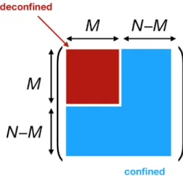
Figure 1. Pictorial representation of partial deconfinement for gauge and adjoint matter degrees of freedom. Only the M × M -block shown in red is excited. This picture is taken from ref. [4]. In this figure, one specific embedding of SU(M ) into SU(N) is shown.

numerical evidence. Then, in section 4 we move on to investigate the nonperturbative Yang-Mills matrix model, which is the original target of our study. The goal is to establish the coexistence of the confined and deconfined sectors in the strongly-interacting theory.

For this purpose we will determine whether the features of the master field we discovered in the Gaussian matrix model can be applied to the field configurations in our target theory. If that is the case, we can demonstrate that the partially-deconfined phase is an intermediate phase in the confinement/deconfinement transition even at strong coupling. In section 5 we conclude the paper with some discussions regarding the future applications.

2 Review of partial deconfinement

We already mentioned in the introduction that partial deconfinement is related to phase coexistence in color space. As such, it can be seen as a phenomenon characterized by deconfinement of an SU(M ) subgroup within the SU(N ) gauge group of a large-N gauge theory. In this section, we start with a formal definition, which can be applied to any large-N gauge theory, including strongly-coupled theories, without introducing any new concept which could be confusing to the readers. Moreover, we provide explicit examples to clarify the physical meaning behind the formal definition: first, the motivation from the gravity side in section 2.1, then an intuitive picture in the gauge theory side in section 2.2, and lastly, the BEC-confinement correspondence which makes the meaning of the formal definition clear in section 2.3.

For the formal definition we use the distribution of the phases of the Polyakov line.

In gauge theories, the Polyakov line is defined by P e ⁱ R

0

dtA

, where P stands for path

ordering. This is a N ×N unitary matrix, and the eigenvalues are written as e ^iθ

, · · · , e ^iθ

,

where the phases θ ₁ , · · · , θ _N lie between −π and +π. At large N , the phases are described

by the distribution function ρ(θ) which is normalized as ^R _−π ^π dθρ(θ) = 1. By using ρ(θ),

JHEP02(2021)004

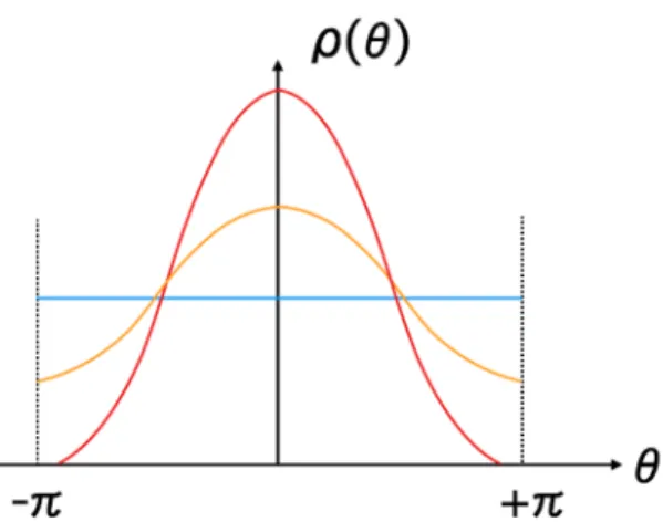
Figure 2. The distributions of the Polyakov line phases in each phase. The blue, orange and red lines are the completely-confined, partially-deconfined and completely-deconfined phases, re- spectively. The specific form of the distribution function ρ(θ) for the partially and completely deconfined phases depends on the theory under consideration.

the completely-confined phase, partially-deconfined phase (equivalently, partially-confined phase) and completely-deconfined phase are defined as follows [6]: ²

• The completely-confined phase refers to an equilibrium state with the uniform phase distribution, ρ(θ) = _2π ¹ . See blue line in figure 2. Note that this is the state which is traditionally called simply the ‘confined phase’.

• The partially-deconfined phase refers to an equilibrium state with the nonuniform phase distribution which is strictly positive, ρ(θ) > 0. See orange line in figure 2.

• The completely-deconfined phase refers to an equilibrium state with the nonuniform phase distribution which is zero in a finite range, in other words it is the ‘gapped’

eigenvalue distribution. See red line in figure 2; there is a gap in the distribution around θ = ±π.

Note that, because this definition does not refer to the center symmetry, it can also be applied to theories without center symmetry, such as the N f -flavor large-N c QCD with N _f /N c finite. (In fact, we believe that partial-deconfinement applies to a rather broad range of theories.) The actual physical meaning of partial deconfinement is not immediately clear from this formal definition. To illustrate it let us focus on the behavior of color degrees of freedom. As depicted in figure 1, two phases — confined and deconfined — coexist

2

The definition provided here requires to strictly take the large-N limit. At the qualitative level, the same picture can be valid at finite N . Imagine that we put finite amount of water in our freezer. We do not have to take the infinite-volume limit in order to see the coexistence of liquid phase and solid phase.

Of course, it is not clear whether atoms at the interface of two phases belong to solid or liquid, but it is a

minor correction to the phase-coexistence picture. Exactly the same situation can be realized at finite N,

namely most colors are in the confined sector or deconfined sector, but some colors may be somewhere in

between. In any event, the large-N limit is needed for a formal definition, so we will focus on the large-N

limit in this paper.

JHEP02(2021)004

in the space of colors [1–6]. The readers may wonder why we consider the possibility of such a seemingly-exotic phase, and how it is related to the formal definition given above.

Therefore, we will provide an extensive review below.

2.1 Motivation from gravity

Partial deconfinement has been originally proposed in order to solve a few puzzles asso- ciated with the confinement/deconfinement phase transition of gauge theories in light of the gauge/gravity duality. In particular, the original motivation [1] was to explain how the gauge/gravity duality relates the thermodynamics of gauge theories to the physics of black holes: this is a very nontrivial problem studied by several papers in the literature, as we discuss below.

The clearest example of the connection between thermal phase transitions in gauge the- ories and black holes can be seen in the duality between the thermodynamics of the 4d N = 4 super Yang-Mills theory (SYM) and the type IIB superstring theory on AdS ₅ ×S ⁵ [10].

In this duality, the confined and deconfined phases on the gauge theory side are dual to the thermal AdS geometry and the ‘large’ black hole in AdS space, respectively. In the canonical ensemble, these two phases are separated by a first order phase transition. This transition is called the Hawking-Page transition.

It was immediately realized that between these two phases there must be an inter- mediate region. From the gravity side of the duality, this is simply a very small black hole, which is approximately the ten-dimensional Schwarzschild black hole [15, 16]. The energy of this small black hole scales as E ∼ N ² T ⁻⁷ , where N ² corresponds to the inverse of the Newton constant. This is a stable physical state in the microcanonical ensemble. ³ Schwarzschild black holes with negative specific heat are more realistic than charged black holes such as the ‘large’ black holes in AdS, which have positive specific heat. Therefore, from the physics point of view, it is important to understand this intermediate phase.

One of the “puzzles” is how to interpret this small black hole state on the gauge side of the duality. In fact, how can a healthy quantum field theory lead to a stable state with a negative specific heat? Partial deconfinement gives a natural answer to this problem [1], introducing a new phase with negative specific heat in thermal phase transitions. The small deconfined sector is regarded as a small black hole, just in the same way as a large deconfined sector — completely deconfined phase — is regarded as a ‘large’ black hole.

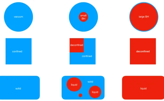
(cf. the top and middle rows in figure 3.) Similar phases with negative specific heat are predicted for other theories too. For example, the D0-brane quantum mechanics [7, 8]

is expected to describe the Schwarzschild black hole in eleven dimensions at very low temperature [20]: such phase would also be understood as a partially-deconfined phase.

3

Precisely speaking, the phase diagram is a little bit more complicated. Below a certain energy, the

large BH (wrapping on S

) has a negative specific heat. In a certain energy range, both the large BH

with negative specific heat and the small BH can be entropy maxima in the microcanonical ensemble. At

some energy the large BH solution becomes unstable against the localization along S

, analogous to the

Gregory-Laflamme transition between black hole and black string. The details of this phase transition have

not been fully understood yet. There are attempts to construct gravity solutions connecting the two phases

(e.g. ref. [18]), and a proposal regarding the gauge theory description [19]. Our numerical analyses in this

paper are not precise enough to see such fine structure, even if it exists.

JHEP02(2021)004

vacuum small large BH

BH

confined deconfined

confined deconfined

solid

liquid

liquid solid

liquid

Figure 3. Analogy between three phases in string theory in AdS space (top), Yang-Mills theory (middle) and water (bottom). Each column represent a different phase. The two-phase coexistence is shown in the center column. The two-phase coexistence in color space can take place even when the order of phase transition is not one. As explicit examples, see ref. [5].

In the context of holography with weakly-curved gravity description, the partially- deconfined phase has negative specific heat. However in more generic gauge theories it is not necessarily the case [3–5], as we will see in section 2.2.

2.2 Intuitive picture

While partial deconfinement seems like an original and natural explanation for the physics

of the small black hole, it was conjectured to be a general mechanism at work in many

theories [2, 3]. For example, it has been analytically proven in several weakly coupled

theories [4–6], starting from seminal papers [16, 21]. These pioneering papers pointed out

that the confinement/deconfinement transition characterized by a jump of the energy and

entropy can exist even in the weak-coupling limit — it can be kinematical, rather than

dynamical — and the intermediate phase resembling the small black hole can exist in gen-

eral. This intermediate phase lies between the Hagedorn transition and the Gross-Witten-

Wadia (GWW) transition [16]. Those transitions are characterized by the distribution of

the phases of the Polyakov line, ρ(θ). At the Hagedorn transition, ρ(θ) changes from uni-

form (ρ(θ) = _2π ¹ ) to non-uniform. At the GWW transition, a gap is formed, namely ρ(θ)

becomes zero in a finite range of θ above the GWW point. Even large-N QCD could have

such an intermediate phase [22] and it appears to be similar to the cross-over region of real

QCD with N = 3. Namely, the GWW transition has to exist, and as we will explain fur-

ther in section 2.3, the GWW transition is naturally identified with the transition from the

partially-deconfined phase to the completely-deconfined phase. At weak coupling, explicit

analytic calculations [5, 22] show a cross-over-like behavior with a third order GWW phase

JHEP02(2021)004

transition (and hence, it is not really cross-over). Partial deconfinement gives a precise physical interpretation to this phase [5].

One way to approach partial deconfinement is to analyze the thermodynamics of large- N gauge theories from the point of view of the microcanonical ensemble [3–5]. In the microcanonical ensemble, the energy E is varied as a parameter, and the entropy S is maximized at each fixed energy. In the confining phase, E and S are of order N ⁰ , up to the zero-point energy, while in the deconfining phase they are of order N ² . This is simply due to the counting of degrees of freedom. In QCD language, we would refer to them as hadrons/glueballs and quarks/gluons. Now we consider a specific value of the energy E = N ² , where is a small but order N ⁰ number, such as 0.1 or 10 ⁻¹⁰⁰ . This is a per- fectly reasonable choice because the energy can be varied continuously. On the other hand, a question arises: what kind of phase is realizing this specific energy? It cannot be the con- fined phase, because the energy is too large and it cannot be the deconfined phase, because the energy is too small. The answer is the partially-deconfined phase with M ∼ √

N . In many theories, including QCD, the canonical and microcanonical ensemble give the same result. The story becomes slightly intricate for systems exhibiting a first-order phase transition in the canonical ensemble, as we will explain in section 2.4. It is worth noting that unless the volume of ordinary space is sufficiently large, the microcanonical ensemble is a physically more realistic setup than the canonical ensemble. This is because the canonical ensemble is typically derived from the microcanonical ensemble as follows. Firstly, let us consider an isolated system in which the energy is conserved, The microcanonical ensemble gives a reasonable statistical description of such a system. If the space is sufficiently large, the system can be divided into a small sub-system and a large heat bath which are in thermal equilibrium. Then the small sub-system is described by the canonical ensemble, with the temperature set by the heat bath. By construction, this derivation of the canonical ensemble assumes sufficiently large spatial volume, and hence, is not applicable to a small volume.

Although partial deconfinement has been discovered only recently, from the discussion above it does not look exotic. Another way to approach it is to recall the first-order transition in a locally interacting system — i.e. the transition between the liquid and solid phases of water — and generalizing it to a system with nonlocal interactions. In the canonical ensemble, water exhibits a first-order phase transition at the temperature of 0 ^◦ C and pressure of 1 atmosphere. In the microcanonical ensemble, depending on the energy E the amount of liquid and solid phases change, because of the latent heat at the transition temperature. When E is small/large the completely solid/liquid phase is observed, while in the intermediate range a mixture of two phases appears. (cf. the bottom row of figure 3.) Equivalently, the mixture of two phases is realized when the energy is not sufficiently small to be in the completely solid phase, and not sufficiently large to be in the completely liquid phase. The temperature remains fixed because of the short-range nature of the interactions:

as long as the interaction at the interface of two phases can be ignored, the temperature cannot change.

A similar mechanism can exist for the gauge theory phase transition introduced above.

In the space of color degrees of freedom two phases — confined and deconfined — can

JHEP02(2021)004

coexist. However, because the interaction between the color degrees of freedom is all- to-all, the temperature can change in a nontrivial way depending on the details of the theory. Pictorially we can visualize three possible patterns as shown in figure 4. The blue, orange, and red lines represent the completely confined phase, partially-deconfined phase (or equivalently, partially-confined phase) and completely deconfined phase. These three phases are the counterparts, in color space, of the solid, mixture and liquid phases, respectively. Let us analyze each pattern individually:

• The center panel in figure 4 would be the easiest one to understand. The Gaussian matrix model studied in section 3 belongs to this class. The temperature does not change, similarly to the case of the mixture of liquid water and ice.

• The Yang-Mills matrix model discussed in section 4 is similar to the left panel in figure 4. In this case, the partially-deconfined phase has a negative specific heat. In the canonical ensemble such phase is not favored thermodynamically and to empha- size this feature we used a dotted line. Strongly coupled 4d N = 4 Yang-Mills and pure Yang-Mills belong to this class too. Depending on the geometry of the ordinary space, instability can set in even in the microcanonical ensemble (see section 2.4 for the details).

In the above example of liquid and solid water, the local nature of the interaction makes the notion of ‘separation into two phases’ easily understandable, because the interaction between the liquid and solid at the interface of two phases is usually negligible. The same holds in the weak-coupling limit of large-N gauge theories, and the separation to confined and deconfined sectors can be proven precisely [4, 5]. See section 3 for an example of this kind. There, a Gaussian matrix model with gauge-singlet constraint is considered. The dynamical degrees of freedom are harmonic oscillators, and in the confined sector they remain in the ground state, while in the deconfined sector they are excited. Note that, even in the weak-coupling limit, the temperature dependence is not necessarily like in the second panel of figure 4. Indeed, large-N QCD with N f flavor, with ^N _N

fixed, shows a nontrivial temperature dependence like the third panel of figure 4, due to the interplay between the number of deconfined color degrees of freedom and the number of deconfined flavor degrees of freedom [5]. With the interaction, the nature of deconfined and confined phases can be modified, but we expect the coexistence of two phases can persist. This point is elaborated more in section 2.3, and also, numerically studied in this paper.

It can also be instructive to consider possible objections to the picture presented by partial deconfinement. For example, it can be objected that the phase separation should only take place in ordinary space and not in the internal space of color degrees of freedom.

However, it is true that the confinement/deconfinement transition can take place even in matrix models where the ordinary space does not exist by definition. In these cases the phase separation can happen only in the internal ‘space’ for these theories. Section 2.4 contains more details about this point.

Another objection would be to have all the color degrees of freedom get mildly excited

and not separate into distinct groups representing the confined and deconfined phases. In

JHEP02(2021)004

Figure 4. Three basic patterns of T -dependence of M [3]. The blue, orange and red lines are the completely confined, partially-deconfined and completely deconfined phases, respectively. [Left]

First-order transition with hysteresis, e.g. strongly coupled 4d N = 4 super Yang-Mills theory on S

, and the Yang-Mills matrix model studied in section 4. [Middle] First-order transition without hysteresis, e.g. free Yang-Mills and Gaussian matrix model studied in section 3. [Right] Non-first- order transition, e.g. large-N QCD [22].

the case of water this possibility is forbidden because of the finite latent heat. In the case of the confinement/deconfinement transition we recall that it can take place even in the weak-coupling limit [16, 21]. The simplest example is the gauged Gaussian matrix model where the color degrees of freedom are just quantum harmonic oscillators with quantized excitation levels. They cannot be ‘mildly’ excited precisely because of quantization: the discreteness of the energy spectrum plays the same role as the latent heat.

A third objection can be raised about the SU(M ) block structure of the deconfined sector of partial deconfinement. We could say that there might be other arrangements of the excited degrees of freedom. However, intuitively, since we are maximizing the entropy at fixed energy, it is natural to expect that the solution of such an extremization problem preserves a large symmetry. A more precise argument can be made by using the equivalence between color confinement at large N and Bose-Einstein condensation [6], as we will see in section 2.3.

2.3 BEC-confinement correspondence and meaning of Polyakov line

In order to understand the precise meaning of partial deconfinement, a tight connec- tion [6] between color confinement in large-N gauge theory and Bose-Einstein condensation (BEC) [25] plays a crucial role.

In the analyses in the weak-coupling limit, it was found that the size of the deconfined sector M can be read off from the distribution of the phases of the Polyakov line as [3–5]

minimum of ρ(θ) = 1 2π

1 − M

N

. (2.1)

The mechanism underlying this correspondence was clarified by identifying a natural — in retrospect, almost trivial — connection between BEC and confinement at large N [6]. In order to make this paper self-contained, let us repeat the argument presented in ref. [6].

Let us consider the system of N indistinguishable bosons in R ^d , trapped in the har-

monic potential. There are N harmonic oscillators ~ x ₁ , · · · , ~ x _N consisting of d-components,

JHEP02(2021)004

described by the Hamiltonian H =

N

X

c=1

~ p _c ²

2m + mω ² 2 ~ x _c ²

!

. (2.2)

The indistinguishability of the particles, which leads to Bose-Einstein statistics, can be incorporated as the redundancy under the S _N -permutation symmetry. Therefore, this sys- tem describes the S _N -gauged quantum mechanics of N -component vectors. The extended Hilbert space containing non-gauge-invariant states is spanned by the standard Fock states,

|~ n 1 , ~ n 2 , · · · , ~ n N i ≡

d

Y

i=1

a ˆ ^†n _i1

√ n i1 ! a ˆ ^†n _i2

√ n i2 ! · · · a ˆ ^†n _iN

√ n iN ! |0i, (2.3)

and the physical, gauge-singlet states are defined as the S _N -permutation-invariant states.

The partition function is given by [26]

Z = ^X

g∈G

Tr ˆ ge ^{−β H ˆ} , (2.4)

where G = S _N is the gauge group and ˆ g is a unitary operator acting on the Hilbert space corresponding to the group element g ∈ G. The trace is taken over |~ n 1 , ~ n 2 , · · · , ~ n N i defined by eq. (2.3). The insertion of ˆ g leads to the projection to the gauge-invariant Hilbert space, after the sum over the gauge group G is taken. More explicitly,

Z = ^X

g∈G

X

~ n

,···,~ n

h~ n 1 , · · · , ~ n N |ˆ ge ^{−β H ˆ} |~ n 1 , · · · , ~ n N i

= ^X

~ n

,··· ,~ n

e ^−β ( E

+···+E

) ^X

g∈S

h~ n 1 , · · · , ~ n N |ˆ g|~ n 1 , · · · , ~ n N i

= ^X

~ n

,··· ,~ n

e ^−β ( E

+···+E

) ^X

g∈S

h~ n 1 , · · · , ~ n N |~ n _g(1) , · · · , ~ n _{g(N )} i. (2.5) For generic excited states, all N particles are in different states, and only g = 1 contributes.

On the other hand, for the ground state | ~ 0, ~ 0, · · · , ~ 0i all elements g ∈ G give the same contribution, which leads to an enhancement by a factor N !. Equivalently, generic states are suppressed by a factor N ! compared to the ground state. As identified by Einstein, this is the cause of Bose-Einstein condensation.

The argument above shows how we can define the gauge-singlet condition explicitely.

As such, we could extend that reasoning to different gauge groups, for example by replac- ing G with a more generic gauge group such as SU(N ) and by considering a more generic field content: there is an enhancement factor (the volume of the gauge group) associated with the ground state (the confined phase). We have seen that the operator ˆ g implements the gauge transformation in the Hilbert space corresponding to a group element g ∈ G.

For the SU(N ) group this element g is nothing but the Polyakov line. Based on this

correspondence, the permutation matrix g in (2.4) and (2.5) for the system of identical

bosons will define the Polyakov line in a natural way [6]. In order to determine the phase

distribution, we look at permutation matrices which leave a typical state contributing

JHEP02(2021)004

to thermodynamics unchanged. When the BEC is formed, long cyclic permutations ex- changing the particles in BEC become dominant [26], and then the off-diagonal long-range order (ODLRO) appears [27]. In terms of the Polyakov line, long cyclic permutations contribute to the constant offset in the distribution function ρ(θ), and the relation (2.1) follows [6]. When BEC is formed, the constant offset becomes nonzero; this is the analogue of the Gross-Witten-Wadia phase transition associated with deconfinement [16] (see also section 3). The same logic applies to generic gauge theories as well. This is the reason why the constant distribution of the Polyakov line phases is a good indicator of confinement.

Note that we can go beyond conventional wisdom: even when the phase distribution is not uniform, we can separate the constant offset and non-uniform part. Namely,

ρ(θ) = C + ˜ ρ(θ), (2.6)

where C ≥ 0 is the minimum of ρ(θ) and ˜ ρ(θ) is a non-constant distribution whose minimum is zero. This C is related to M as

C = 1 2π

1 − M

N

. (2.7)

Hence we can fix the ordering of θ i ’s such that θ 1 , · · · , θ _M give the nonuniform part ˜ ρ(θ), while θ _M+1 , · · · , θ _N lead to the constant part C. This separation should correspond to the splitting of the matrix degrees of freedom to the confined and deconfined sectors, and if we see other fields, the phase separation pictorially shown in figure 1 has to hold.

As proposed by Fritz London [28], superfluid helium is understood as BEC. Although BEC was first discovered at vanishing coupling, it can actually take place even at strong coupling. This historically famous fact, together with intriguing similarities of various quantum field theories at weak and strong coupling (see e.g. [13, 29]), motivate our op- timism that partial deconfinement can be valid even at strong coupling. We will give numerical evidence supporting this optimism later in this paper.

2.4 Remarks on negative specific heat

Here we summarize some remarks about the partially-deconfined phase in the case where it has negative specific heat. We refer again to the leftmost panel of figure 4. If the volume of the ordinary space is large, the phase with a negative specific heat is not stable. Any small perturbation can trigger a decay to the co-existence of a completely confined and a completely deconfined phases. This is not necessarily the case if the volume is small and finite. In the case of matrix models, such instability cannot exist by definition, because there is no ordinary space by definition. Moreover, 4d N = 4 super Yang-Mills on S ³ does not have such instability. The partially-deconfined phase in 4d N = 4 super Yang-Mills on S ³ is dual to the small black hole phase, which does not have such instability. ⁴ It can also be understood via a simple dimensional analysis as follows. For the coexistence of two phases in the ordinary space to appear, the radius of S ³ , which we call r, has to be sufficiently larger than the typical length scale of the system, which is the inverse of the

4

There is a subtlety regarding this point, near the phase transition associated with the localization on

the S

; see 2.1.

JHEP02(2021)004

temperature of the partially-deconfined phase, β. However β and r are of the same order, as explained in ref. [10].

When the specific heat is negative, the partially-deconfined phase sits at the maximum of the free energy in the canonical ensemble [3]. The completely confined and completely deconfined phases are the minima of the free energy. The difference of free energy be- tween the minima and the maximum between them is of order N ² and the tunneling is parametrically suppressed at large N . In this way, the local minima is completely stabi- lized at large N , even when it is not the global minimum. This is very different from the metastable states in the locally interacting systems, such as the supercooled water: even in the thermodynamic limit (large volume) already a small perturbation can destabilize the supercooled water.

3 Partial deconfinement: the Gaussian matrix model

Let us consider the gauged Gaussian matrix model. The action is given by eq. (1.2). This model is analytically solvable [16, 21] and partial deconfinement has been introduced for the phase transition in refs. [2, 4]. We start from this solvable case in order to analyze how partial deconfinement manifests itself in the path integral formalism.

In the previous section we already mentioned that the Gaussian matrix model has a confinement/deconfinement phase transition which is of first order without hysteresis in the canonical ensemble (the center panel of figure 4). The critical temperature is T = T c = _log ¹ _d . In the canonical ensemble, at T = T _c , the energy E and entropy S jump from order N ⁰ to order N ² , while the Polyakov loop P = _N ¹ TrPe ^{i R}

β

0

dtA

jumps from 0 to ¹ ₂ (see figure 2 of ref. [4].) We also fix the center symmetry ambiguity in the phase of the Polyakov loop by setting P = |P | for the remainder of this paper.

As functions of the Polyakov loop, the energy and entropy are expressed as ⁵ E| _{T =T}

c

≡ N β

Z dt ^X

I

TrX _I ² T =T

= d

2 N ² + N ² P ² (3.1) and

S| _{T =T}

c

= log d · N ² P ² . (3.2)

As mentioned above, at the critical temperature P can take any value from 0 to ¹ ₂ . There- fore, up to the zero-point energy ^d ₂ N ² , the energy E and entropy S changes from N ⁰ to N ² , as P changes from 0 to ¹ ₂ . The distribution of the phases of the Polyakov line is

ρ ^(P) (θ)

T =T

= 1

2π (1 + 2P cos θ) . (3.3)

The free energy F = E − T S does not depend on P : F | _{T =T}

c

= d

2 N ² . (3.4)

5

The derivation of eqs. (3.1), (3.2) and (3.3) can be found in section 3 and appendix A.1 of ref. [4].

JHEP02(2021)004

Hence all values of P contribute equally to the canonical partition function. Essentially the same results hold for various weakly-coupled theories [16, 21].

So far we have introduced important relations for the Gaussian matrix model quantities and we want to relate them to partial deconfinement, following the findings in ref. [4]. At T = T c , the size of the deconfined sector M jumps from M = 0 to M = N . This size can be read off from the distribution of the phases of the Polyakov line, as explained in section 2.3. In the case of the Gaussian matrix model, this relation simplifies to [4]

P = M

2N . (3.5)

This equation connects an observable of the system (P ) to the amount of deconfined degrees of freedom M/N. Below, we will explain how the separation to two phases (confined and deconfined sectors) can be seen by using this M . In section 3.1, the explicit separation in terms of the quantum states is explained as well.

It follows that the distribution of the phases of the Polyakov loop in eq. (3.3) can be written as

ρ ^(P) (θ)

T =T

= 1 2π

1 + M

N cos θ

. (3.6)

Similarly, for the energy E and the entropy S, we can write E| _{T =T}

c

≡ N β

Z dt ^X

I

TrX _I ² = d

2 N ² + M ²

4 , (3.7)

S| _{T =T}

c

= log d

4 M ² . (3.8)

Note that these relations are valid only at the phase transition temperature T = T c

where partial deconfinement takes place. Later in this paper, when we perform the numerical analysis at large but finite N , we determine M from eq. (3.5) by imposing 2N P ∈ [M − ¹ ₂ , M + ¹ ₂ ].

While the energy and the entropy have a discontinuity at T = T _c in the canonical ensemble, that is not the case for the microcanonical ensemble where the entropy is max- imized for each fixed system energy. Therefore, it follows that M can be defined by the energy itself through eq. (3.7). Moreover, in the microcanonical ensemble there are two phase transitions: one from M = 0 to M > 0 and one from M < N to M = N . They are called the Hagedorn transition and Gross-Witten-Wadia (GWW) transition, respectively.

In order to understand the nature of the states in the microcanonical ensemble, let us rewrite eqs. (3.6), (3.7) and (3.8) as follows:

ρ ^(P) (θ)

T =T

=

1 − M N

· 1 2π + M

N · 1 + cos θ

2π , (3.9)

E| _{T =T}

c

= d

2 (N ² − M ² ) + d

2 + 1 4

M ² , (3.10)

S| _{T =T}

c

= 0 · (N ² − M ² ) + log d

4 M ² . (3.11)

This way we can separate clearly two different contributions that get summed. For each

equation, the first term of the sum is interpreted as the contribution of the ground state,

JHEP02(2021)004

while the second term is just the value of each observable for an SU(M ) theory at the GWW-transition point (only M degrees of freedom can be excited). Partial deconfinement shown in figure 1 naturally explains this M-dependence.

One objection to this idea would be that figure 1 does not look gauge invariant. Hence, in order to prove partial deconfinement in a gauge-invariant manner, we first show in section 3.1 the explicit construction of the gauge-singlet states in the Hilbert space from the Hamiltonian formalism. Then, in section 3.2, we consider the path integral formalism, which is used in the lattice Monte Carlo simulation and we discuss the properties of the master field.

3.1 The Hamiltonian formalism

Following ref. [4], in the large-N limit, we explicitly construct the states governing ther- modynamics in the gauged Gaussian matrix model. The Hamiltonian is

H ˆ = 1

2 Tr P ˆ _I ² + ˆ X _I ² . (3.12) The creation and annihilation operators are defined as A ˆ ^† _I = ^{√ 1}

2

X ˆ I − i P ˆ I

and A ˆ _I = ^{√ 1}

2

X ˆ _I + i P ˆ _I . The ground state is the Fock vacuum |0i which is annihilated by all annihilation operators:

A ˆ _I |0i = 0. (3.13)

The physical states have to be gauge singlets, e.g.

Tr A ˆ ^† _I A ˆ ^† _J A ˆ ^† _K · · · |0i =

N

X

i,j,k,l···=1

A ˆ ^† _I,ij A ˆ ^† _J,jk A ˆ ^† _K,kl · · · |0i (3.14)

Let ˆ A ^†0 _I be the truncation of ˆ A ^† _I to the SU(M)-part. We can construct the states which are SU(M)-invariant but not SU(N )-invariant as

Tr A ˆ ^†0 _I A ˆ ^†0 _J A ˆ ^†0 _K · · · |0i =

M

X

i,j,k,l···=1

A ˆ ^† _I,ij A ˆ ^† _J,jk A ˆ ^† _K,kl · · · |0i. (3.15)

Note that the indices in the sum run from 1 to M (not N). Such states are essentially the same as the states in the SU(M ) theory. By collecting such states with the energy given by eq. (3.10), we can explain the entropy in eq. (3.11) and the distribution of the phases of the Polyakov loop of eq. (3.9). Note that the states above are not invariant under the full SU(N ) symmetry. In order to obtain the SU(N )-invariant states, we consider all possible embeddings of SU(M) into SU(N ) and take a linear combination. Namely, we consider

√ 1 N

Z

SU(N)

dU U (|E; SU(M )i) , (3.16)

where |E; SU(M )i is SU(M )-invariant but not SU(N )-invariant, U represents gauge trans-

formations, N is the normalization factor, and the integral is taken over all SU(N ) gauge

transformations. Such SU(N )-symmetrized states dominate the thermodynamics.

JHEP02(2021)004

At large N , the gauge-invariant, SU(N )-symmetrized state in eq. (3.16) is indistin- guishable from the state with a particular embedding of SU(M) such as eq. (3.15) in the following sense. Let |SU(M )i ₁ be the state with a particular embedding, and |SU(M )i ₂ be a state obtained by acting with a certain unitary transformation on |SU(M)i ₁ . For example, |SU(M)i ₁ has excitations only in the upper-left M × M block, while |SU(M )i ₂ has excitations only in the lower-right M × M block. Let ˆ O be a gauge-invariant operator which is a polynomial of O(N ⁰ ) matrices. We consider these ‘short’ operators because they do not change the energy too much and we want to study the properties of the states with energy of order N ² . ⁶ Then, ₂ hSU(M)| O|SU(M ˆ )i ₁ = 0, because to connect |SU(M )i ₁ to

|SU(M )i ₂ it is necessary to act with O(N ² ) creation and annihilation operators. This is essentially a super-selection rule: different embeddings of SU(M ) to SU(N ) belong to dif- ferent super-selection sectors. This ‘superselection’ can work even when the embeddings are very close. Suppose the upper-left M × M block is deconfined in |SU(M)i ₁ , and |SU(M )i ₂ is obtained by permuting the M -th and M +1-th rows and columns. Those two embeddings appear almost identical, but to connect |SU(M )i ₁ and |SU(M )i ₂ the length of the operator O ˆ has to be of order N ¹ . More generally, let V be a generator of SU(N )/SU(M ), whose norm

q

Tr(V V ^† ) is small but of order N ⁰ , say 0.1 × N ⁰ . Then, if |SU(M )i ₂ is obtained by acting the SU(N ) transformation e ^iV , then ₂ hSU(M )| O|SU(M ˆ )i ₁ = 0 in the large-N limit with fixed ^M _N . Hence whether we use a particular embedding or a superposition of all embeddings, we get the same expectation value for ˆ O.

3.2 The path integral formalism and lattice Monte Carlo

So far we only reviewed how partial deconfinement can be seen in terms of the states in the Hamiltonian formalism, following the results in ref. [4]. Next, we consider the path integral formalism which is used in the lattice Monte Carlo simulations of this paper.

3.2.1 Ensemble properties and master field

An important remark is that the field configurations in the path integral formalism do not have a simple connection to the quantum states in the Hilbert space, other than the fact that the expectation values of gauge-invariant observables agree. This makes the connection with partial deconfinement a little bit more intricate, in particular when trying to analyze the configurations obtained in lattice Monte Carlo simulations. A typical misunderstanding would be “the lattice configurations are the wave functions describing specific states in the Hilbert space”; the absence of such a simple connection would be illuminated by noting that lattice configurations have to be averaged in order to obtain the expectation values, unlike the wave function.

At large N , there is a simplification: statistical fluctuations are suppressed at leading order, and we can expect the master field [30] to appear and dominate the path inte- gral. ⁷ Note that the master field is not the wave function representing the state in the

6

The counterpart of this in the case of a finite-N theory at large volume is to consider only the operators with a compact support, in order to make sense of the boundary conditions.

7

For a review of the master field, the readers can refer to ref. [31].

JHEP02(2021)004

Hilbert space. Still, we can find characteristic features of the master field describing the partially-deconfined phase, by making a ‘mapping’ between typical states and the master field configuration (typical lattice configurations). Our strategy is to confirm those features by lattice simulation.

In this paper, we refer to the master field as a lattice configuration in the Euclidean path integral of the theory at large N which gives the correct expectation values for properly normalized quantities such as E/N ² to leading order in the expansion with respect to 1/N : hf(A _t , X _I )i = f A ^(master) _t , X _I ^(master) (at large N ). (3.17) Here f can be any properly normalized gauge-invariant quantity following the ’t Hooft scaling, as long as it does not affect the dominant configuration in the path integral, similarly to the operator ˆ O considered in section 3.1. We need to understand the features of the master field describing the partially deconfined phase in the Gaussian matrix model.

Then we can start looking for the master field in nontrivial theories such as the Yang-Mills matrix model. ⁸

Because lattice Monte Carlo simulations are based on importance sampling, the sample-by-sample fluctuations of the properly normalized quantities (e.g. E/N ² , which is of order N ⁰ in the large-N limit) are suppressed as N becomes larger. In the strict large-N limit, configurations appearing in lattice simulations can be identified with the master field. However, in actual simulations, we can only study large but finite N values.

To learn about the master field in lattice simulations, we simply study the features of con- figurations sampled by the Markov Chain Monte Carlo (MCMC) algorithm, at sufficiently large N , identifying them with master fields.

In the standard lattice Monte Carlo simulations, the canonical ensemble is obtained.

The canonical partition function can be obtained from the microcanonical ensemble as Z (β) =

Z

dEΩ(E)e ^−βE = Z

dEe −β(E−T S(E))

, (3.18)

where Ω(E) = e ^S(E) is the density of states at energy E. Near the first-order transition, as a function of E, ‘free energy’ E −T S(E) can have multiple saddles. Those saddles correspond to the maxima of the entropy at the energy E, where the microcanonical temperature dS

dE

−1

equals the canonical temperature T. ⁹ We assume that the microcanonical ensemble can be represented by one master field at each energy E, and expect that each saddle point has a corresponding master field. In the case of the Gaussian matrix model at T = T c , any M between 0 and N minimizes the free energy, and hence, we need to treat all values of M separately. We expect there is a master field for each M , and we identify them as the dominant configurations for a given (T, M ) pair. This can be found using numerical lattice simulations.

8

A few comments regarding the master field in the completely confined and completely deconfined phases in four-dimensional pure Yang-Mills theory at N = ∞, in the context of lattice Monte Carlo simulations, can be found in ref. [32].

9

The saddle-point condition

(E −T S ) = 0 leads to 1−T ·

= 0, which is equivalent to

= T .

JHEP02(2021)004

The master field has an ambiguity due to gauge redundancy. In order to eliminate the redundancy, we perform Monte Carlo simulations in the static diagonal gauge. In this gauge, the gauge symmetry is fixed up to S _N permutations. The gauge field takes the form

A t = diag θ 1

β , · · · , θ N

β

, (3.19)

where θ 1 , · · · , θ _N are independent of t, and θ i ∈ [−π, +π). By using them, the Polyakov loop P is expressed as P = _N ^{1 P N} _j=1 e ^iθ

.

The Polyakov loop phases can be divided into two groups:

1. M of them (we can take them to be θ 1 , · · · , θ M without loss of generality) distributed following the density ^1+cos _2π ^θ ;

2. N − M of them (θ _{(N −M)} , · · · , θ _N ) distributed following the density _2π ¹ .

In terms of the Hilbert space, this corresponds to the separation to the deconfined block and the confined block pictorially shown in figure 1 [3, 6]. This subdivision is fixing the residual S _N permutation symmetry further to S _M ×S _{N −M} , where rearrangements inside the two separate groups are indistinguishable for gauge-invariant properties. ¹⁰

We note that in terms of the Euclidean path integral there is still a small residual symmetry. Namely, the same value of θ can appear in both sectors, ¹¹ and the permutation acting on them ¹² does not change the distribution of the Polyakov line phases. As we will see below, this is a feature rather than a bug.

In the rest of this section, we will discuss a few properties of the master field which are related to partial deconfinement. ¹³ Having the application to the Yang-Mills matrix model in mind, we will demonstrate that such properties are visible in lattice configurations.

3.2.2 Distribution of X I,ij

As a simple characterization of the master field, let us consider the distribution of

√

N X I,jj (t), √

2N ReX _I,jk (t) and √

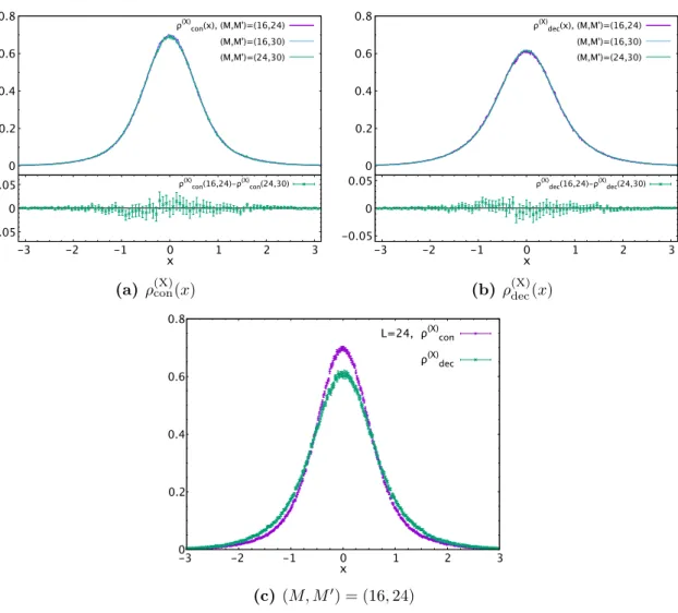
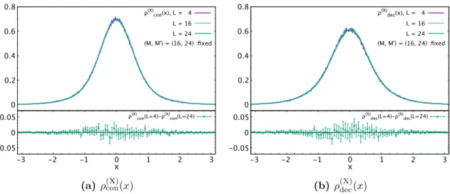
2N ImX _I,jk (t). These are the diagonal and off-diagonal elements of all the scalar hermitean matrices and represent a standard lattice field configu- ration. We collectively denote them as a random variable ‘x’ with distribution ρ ^(X) (x). At T = T c , we want to identify the contributions to this distribution coming from the confined and deconfined sectors. We denote them by ρ ^(X) con (x) and ρ ^(X) _dec (x), respectively. In fact, we expect a very specific form,

ρ ^(X) (x) = 1 − M

N 2 !

· ρ ^(X) _con (x) + M

N 2

· ρ ^(X) _dec (x), (3.20)

10

In fact, such separation is not unique; there is residual symmetry under the exchange of θ’s with the same value in the confined and deconfined sectors. This is not a bug, this is a feature. Our numerical results are consistent with the separation, including the consequence of this ambiguity. See section 3.2.3, especially the description after eq. (3.33), for details.

11

Strictly speaking, at finite N , because of the Faddeev-Popov term associated with the gauge fixing S

= − P

i<j

log ^sin

2

i−θ_j 2

^, θ’s cannot exactly coincide. However in the large-N limit neighboring θ’s can come infinitesimally close.

12

When we permute θ

and θ

, we exchange the i-th and j-th rows and columns of the scalars X

as well.

13

In principle, it should be possible to learn more detailed of the master field. See for example ref. [33].

JHEP02(2021)004

where M is related to P by eq. (3.5), i.e. M = 2P N. From the point of view of partial deconfinement, this relation can readily be understood: the confined and deconfined sectors coexist in the space of color degrees of freedom. On the other hand, without introducing partial deconfinement, this is extremely nontrivial. In order to determine this distribution from lattice configurations at fixed M, we can obtain many samples of x and plot their histogram (for example, we can collect dLN ² = 49152 samples from a d = 2, N = 32, L = 24 configuration, where L is the number of lattice points).

The distribution ρ ^(X) (x) has some interesting properties. The part of the action de- scribing the scalar is

N Z β

0

dt ^X

I

X

j,k

1 2

∂ t X _Ijk − i(θ j − θ k ) β X _Ijk

2

+ |X _Ijk | ²

!

= N Z β

0

dt ^X

I

X

j,k

1 2

(

|∂ _t (ReX Ijk )| ² + 1 + (θ j − θ k ) ² β ²

!

|ReX _Ijk | ²

+ |∂ _t (ImX Ijk )| ² + 1 + (θ j − θ k ) ² β ²

!

|ImX _Ijk | ² )

. (3.21) From this expression, we can see that the distribution of √

2N ReX _I,jk (t) and

√ 2N ImX _I,jk (t) depends only on θ _j − θ _k .

From here on, we focus on T = T c where partial deconfinement takes place, and we consider the SU(M )-partially-deconfined phase. As mentioned before, it is convenient to go to a ‘gauge-fixed’ picture, in which the S _N permutation symmetry is fixed to S _M ×S N−M . It is achieved by separating θ i ’s into two groups, such that θ 1 , · · · , θ M and θ M+1 , · · · , θ N

are distributed as ^1+cos _2π ^θ and _2π ¹ , respectively. If we take the average over j = M +1, · · · , N or k = M + 1, · · · , N , then the distribution of θ j − θ k is uniform, just as in the completely confined phase. In other words, the distribution of x is the same as in the completely confined phase. On the other hand, if we take the average over j, k = 1, · · · , M we see the difference from the confined phase, because θ j − θ k is not uniform. In particular, the energy E defined by eq. (3.7) can be directly related to the second moment of ρ ^(X) (x) by

E =

* N β

Z β 0

dtTrX _I ² +

= dN ² Z

x ² ρ ^(X) (x)dx

= d(N ² − M ² ) Z

x ² ρ ^(X) _con (x)dx + dM ² Z

x ² ρ ^(X) _dec (x)dx, (3.22) where

dM ² Z

x ² ρ ^(X) _dec (x)dx =

* N β

Z β 0

dt ^X

1≤j,k≤M

|X _I,jk | ² +

(3.23) corresponds to the deconfined sector where θ j − θ _k is not uniform, and

d(N ² − M ² ) Z

x ² ρ ^(X) _con (x)dx =

* N β

Z β 0

dt ^X

j≥M+1 or k≥M+1

|X _I,jk | ² +

(3.24)