Policy Research Working Paper 7448
The Effect of Metro Expansions on Air Pollution in Delhi
Deepti Goel Sonam Gupta
Development Economics Vice Presidency Operations and Strategy Team
October 2015
WPS7448
Public Disclosure AuthorizedPublic Disclosure AuthorizedPublic Disclosure AuthorizedPublic Disclosure Authorized
Abstract
The Policy Research Working Paper Series disseminates the findings of work in progress to encourage the exchange of ideas about development issues. An objective of the series is to get the findings out quickly, even if the presentations are less than fully polished. The papers carry the names of the authors and should be cited accordingly. The findings, interpretations, and conclusions expressed in this paper are entirely those of the authors. They do not necessarily represent the views of the International Bank for Reconstruction and Development/World Bank and its affiliated organizations, or those of the Executive Directors of the World Bank or the governments they represent.
Policy Research Working Paper 7448
This paper is a product of the Operations and Strategy Team, Development Economics Vice Presidency. It is part of a larger effort by the World Bank to provide open access to its research and make a contribution to development policy discussions around the world. Policy Research Working Papers are also posted on the Web at http://econ.worldbank.org.
The authors may be contacted at deepti@econdse.org and sgupta@impaqint.com.
The Delhi Metro (DM) is a mass rapid transit system serv- ing the National Capital Region of India. It is also the world’s first rail project to earn carbon credits under the Clean Development Mechanism of the United Nations for reductions in CO2 emissions. Did the DM also lead to local- ized reduction in three transportation source pollutants?
Looking at the period 2004–2006, one of the larger rail
extensions of the DM led to a 34 percent reduction in local- ized CO at a major traffic intersection in the city. Results for NO2 are also suggestive of a decline, while those for PM25 are inconclusive due to missing data. These impacts of pollutant reductions are for the short run. A complete accounting of all long run costs and benefits should be done before building capital intensive metro rail projects.
The Effect of Metro Expansions on Air Pollution in Delhi Deepti Goel and Sonam Gupta
JEL codes: Q5, R4
Keywords: Air pollution, Delhi Metro, urban transport
Deepti Goel (corresponding author) is an assistant professor in the Department of Economics, Delhi School of Economics, University of Delhi, Delhi 110007; her email is deepti@econdse.org. Sonam Gupta is a research associate with IMPAQ International; her email is sgupta@impaqint.com. The authors are grateful to the journal’s referees for their critical feedback that substantially improved the paper. They also thank Mr. Amit Kumar Jain from the Delhi Metro Rail Corporation and Dr. D. D. Basu and Mr. D. C. Jakhwal from the Central Pollution Control Board for their help in obtaining some of the data used in the paper. The authors are also grateful to Shantanu Khanna for his excellent research assistance.
2
The Delhi Metro (DM) is an electric-based mass rapid rail transit system mainly serving the Indian National Capital Territory (NCT) of Delhi. The NCT of Delhi covers an area of 1,483 square kilometers and has a population of 16.8 million people according to the Indian Census of 2011, making it one of the world’s most densely populated cities.1 The DM was introduced in 2002 and since then it is being continually extended within the NCT and adjoining areas. As of 2012, its total route length was 190 kilometers, and annual ridership was 0.7 billion (DMRC 2012).2 In this paper we examine whether this important mode of public transportation has had any impact on air pollution in Delhi. We identify the immediate localized effect of extending the DM rail network on air pollution measured at two different locations within the city: ITO, a major traffic intersection in central Delhi, and Siri Fort, a mainly residential neighborhood in south Delhi.
Air pollution is measured in terms of three criteria pollutants, namely, nitrogen dioxide (NO2), carbon monoxide (CO), and fine particulate matter (PM2.5).
An impact study of the DM on air pollution is important for two reasons.
First, there is substantial scientific evidence on the adverse effects of air pollution on human health. Block et al. (2012) provide a review of epidemiological research that shows the link between air pollution and damage to the central nervous system, which may manifest in the form of decreased cognitive function, low test scores in children, and increased risk of autism and of neurodegenerative diseases such as Parkinson’s and Alzheimer’s. They also cite other studies which show that air pollution causes cardiovascular disease (Brook et al. 2010) and worsens asthma
1. According to a worldwide ranking of cities by City Mayors Statistics, Delhi ranked thirteenth in terms of
population density with 11,050 persons per square kilometer. Mumbai ranked first, and Beijing ranked twelfth, with population densities of 29,650 and 11,500, respectively. The data are compiled from various sources and are the most recent available. Source url: http://www.citymayors.com/statistics/largest-cities-density-125.html. Last accessed on March 31, 2015.
2. As of 2014, the Beijing Subway had a route length of 527 kilometers and annual ridership of 3.4 billion. This information is accessed from Wikipedia. Source url: http://en.wikipedia.org/wiki/Beijing_Subway. Last accessed on March 31, 2015.
3
(Auerbach and Hernandez 2012). Turning to recent research in economics, Tanaka (2015) finds that regulations to curb pollution from coal-based power plants in China led to 3.29 fewer infant deaths per 1000 live births, amounting to a 20 percent reduction in infant mortality rate.3 Ghosh and Mukherji (2014) examine the effect of ambient air quality on children’s respiratory health in urban India and find that a rise in particulate matter significantly increased the risk of respiratory ailments. Arceo-Gomez et al. (2012) provide evidence from Mexico City that a 1 percent increase in particulate matter (PM10) over a year led to a 0.42 percent increase in infant mortality, and the corresponding figure for CO is 0.23 percent.
Currie and Walker (2011) find that exposure to vehicular emissions around toll plazas in the northeastern United States increased the likelihood of premature births and also resulted in low birth weight. Some other studies that document the adverse health consequences of air pollution for the United States include Moretti and Neidell (2011); Lleras-Muney (2010); and Currie, Neidell, and Schmieder (2009).
The second compelling reason for this study is the extent of air pollution in Delhi. According to the World Health Organization’s (WHO) database, Ambient Air Pollution 2014, Delhi is the most polluted city in the world in terms of PM2.5 levels. In 2013, the annual mean concentration of PM2.5 in Delhi was almost twenty times the guideline value prescribed by the WHO.4 The Central Pollution Control Board (CPCB), the national authority responsible for monitoring and managing air
3. Greenstone and Hanna (2014) find that environmental regulations in India have been effective in reducing air pollution. However, in contrast to Tanaka (2009), they find an insignificant impact of reduced air pollution on infant mortality. For reasons discussed in their paper, they advise readers to be cautious when interpreting their result on infant mortality.
4. The WHO guideline for annual mean concentration of PM2.5 is 10 g m/ 3, and in 2013, the annual mean level of PM2.5 in Delhi was198g m/ 3. Notably, Delhi's PM2.5 level far exceeded that of Beijing which was at
56g m/ 3 (Ambient Air Pollution Database 2014, WHO).
4
quality in India, finds that pollution in Delhi is positively associated with lung function deficits and with respiratory ailments (CPCB 2008a; CPCB 2008b).
Guttikunda and Goel (2013) estimate that particulate matter present in Delhi in 2010 led to premature deaths ranging from 7,350 to 16,200 per year and to 6 million asthma attacks per year. As Delhi continues to grow, population and vehicle densities are bound to increase further, making it all the more important to examine whether the expansion of the DM has had an impact on the city’s air quality.
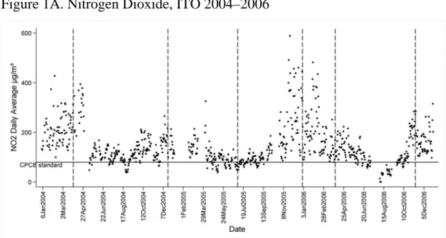
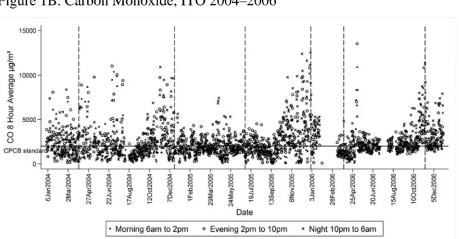
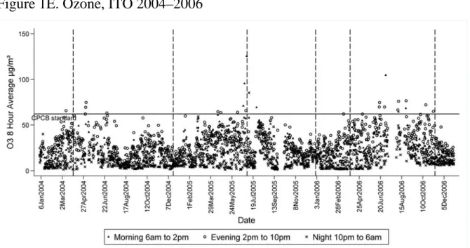
Figures 1A through 1E present the pollution picture at ITO during our study period, 2004 to 2006. Each figure shows the 8- or 24-hour average for a specific pollutant along with the corresponding upper limit prescribed by the CPCB.5 There are some noticeable gaps in each series due to missing observations. In spite of this we see a clear seasonal pattern for nitrogen dioxide (NO2), carbon monoxide (CO), and particulate matter (PM2.5), with their levels being higher in winter (November through January) than in summer (April through June). Further, in the cases of NO2, CO, and PM2.5, there were a large number of occurrences when their levels exceeded prescribed limits, while there were fewer violations for sulphur dioxide (SO2) and ozone (O3). During this period, NO2, CO, and PM2.5, exceeded limits 85, 48, and 78 percent of the time, respectively, while the corresponding figures for
SO2 and O3 were much lower at 3 and 0.1 percent, respectively.6 Given that SO2 and O3 were within permissible limits most of the time, our analysis focuses on
NO2, CO, and PM2.5.
5. Appendix table S1.1 in the supplementary appendix S1 presents the CPCB limits along with those prescribed by the WHO. WHO (2000) maintains that its limits are to be interpreted as guidelines, and individual countries may have different standards based on prevailing exposure levels, and social, economic, and cultural considerations. We measure violations vis-à-vis the CPCB limits, as they should be more relevant within the Indian context.
6. During the same period at Siri Fort, NO2, CO, SO2 andO3, exceeded prescribed limits, 13, 26, 0, and 5 percent of the time, respectively. PM2.5 was not recorded at Siri Fort.
5
Another reason for restricting focus to only these pollutants is that while NO2, CO, and PM2.5 are mainly generated from transportation sources, SO2 and O3 are not. In one of the first pollution inventory studies for Delhi, Gurjar et al. (2004) infer that during their study period (1990–2000), transport sector contributed about 82 percent of nitrogen oxides (NOx),7 and 86 percent of CO. In another study for Delhi conducted in 2007, NEERI (2010) reports that the contribution of vehicles towards NOx, CO, and particulate matter (PM2.5 and PM10) was 18, 58, and 59 percent, respectively. For Delhi in 2010, Guttikunda and Calorie (2012) estimate that 67, 28, and 35 percent of NOx, CO, and PM2.5, respectively, can be attributed to vehicles.8 While there is variation across studies in the exact share of transportation sources in generating these pollutants, all of them report substantial shares. On the other hand, NEERI, and Guttikunda and Calorie, report that vehicular emissions were responsible for 0.3 percent and 3 percent, respectively, of
SO2.9 None of these studies look at O3. However, it is known that O3 is not directly emitted by motor vehicles, but is created through a complicated nonlinear process wherein oxides of nitrogen and volatile organic compounds react together in the presence of sunlight (Sillman, 1999). Thus, of the five pollutants for which we have data, motor vehicles constitute a major and direct source of only three, namely, NO2, CO, and PM2.5. To the extent that one of the main channels through which the DM is likely to affect air pollution is through its impact on overall levels of vehicular emissions, we focus our attention on these three pollutants. Moreover, Delhi is a heavily motorized city,10 and the consequent vehicular emissions are a
7. NOx refers to both nitrogen monoxide (NO) and nitrogen dioxide (NO2).
8. The contribution of vehicles towards particulate matter reported in NEERI (2010) and in Guttikunda and Calorie (2012) includes the contribution of road dust as well.
9. Gurjar et al. (2004) do not report this figure for SO2.
10. Among the 44 reported million-plus cities in India, Delhi had the largest number of registered motor vehicles during 2011–12 with 7.4 million vehicles (TRW 2013). Goel et al. (2015) estimate that of all registered cars and
6 matter of serious concern.
Theoretical research from transport economics (Vickery 1969; Mohring 1972) postulates the existence of two counteracting effects on air pollution from introducing a new mode of public transportation. On the one hand, the introduction of the new mode could increase overall economic activity, which could in turn generate new demand for intracity trips. New demand for travel could also be created if the availability of rapid public transport results in a relocation of residents away from the city-center, for example, if real estate is cheaper in the suburbs leading to longer commutes to work. Such demand that did not exist before the new mode was introduced is referred to as the traffic creation effect. If part of the new demand is met by private means of transport, then ceteris paribus this should add to existing levels of vehicular emissions and increase air pollution.
On the other hand, with the introduction of a new mode of public transportation, commuters who had earlier relied on private means may now switch to the new mode.11 This substitution away from private to public mode of travel is called the traffic diversion effect. Ceteris paribus, the traffic diversion effect should reduce the overall level of vehicular emissions and consequently reduce air pollution. In reality both effects are likely to operate. We hypothesize that the traffic diversion effect is likely to dominate the traffic creation effect in the short run. This is because the processes involved in creating new demand for travel are likely to unfold slowly and over a longer period of time, while the traffic diversion effect can occur almost immediately after the new mode is introduced. Nonetheless, it is
two-wheelers in Delhi in 2011; 59 percent and 42 percent, respectively, are in-use. If we make a very conservative estimate of vehicles in use and assume that only 42 percent of all registered motor vehicles are in use, we get a figure of 3.1 million for in-use vehicles in Delhi. In 2013, the number of in-use vehicles in New York City was 2 million (Department of Motor Vehicles, New York State website; source url: http://dmv.ny.gov/org/about- dmv/statistical-summaries, last accessed on March 31, 2015). Thus, Delhi has at least 55 percent more in-use vehicles than New York City.
11. According to a report by the Delhi Metro Rail Corporation (DMRC, 2008), the DM has already taken the share of 40,000 vehicles.
7 important to verify this empirically.
To be able to attribute changes in a pollutant measure to the DM, we use the Regression Discontinuity (RD) approach. As we explain below, due to the presence of sporadic sources of pollution in Delhi (such as spontaneous burning of waste), this approach is not ideal for short periods of analysis. We therefore rely on a three-year study period and argue that these sporadic sources of pollution cancel each other within this timeframe, resulting in reliable estimates.
Our analysis reveals that soon after some of the larger extensions of the DM there were significant reductions in at least some transportation source pollutants.
Specifically, when we consider our entire study period, 2004–2006, we find that the first extension of the Yellow Line, characterized by the largest surge in metro ridership, resulted in a 34 percent reduction in CO at ITO. Additionally, there is suggestive evidence of a decline in NO2 at ITO due to the introduction of the Blue line. We are unable to say anything conclusive about PM2.5 due to poor quality data on this pollutant.
The rest of the paper is organized as follows. In section I we briefly describe the institution of the DM. The empirical strategy is explained in section II and the data sources are listed in section III. Section IV presents our empirical results and section V places them in the context of existing literature on air pollution. Section VI ends with policy recommendations.
IGENESIS AND EXPANSION OF THE DELHI METRO
The Delhi Metro Rail Corporation Limited (DMRC) was set up in 1995 by the governments of Delhi and India to take over the construction and subsequent operation of the DM. Construction work for the metro began in 1998. The first commercial run took place on December 25, 2002, between Shahdara and Tis Hazari in north Delhi, marking the beginning of operations.
8
The various stages of expansion of the metro rail network were planned keeping in mind the expected demand for transportation from different localities.
The rail lines were first laid in areas with a high population density and where it was felt that the metro would benefit the largest number of people. Subsequent extensions were similarly motivated. Table 1 details the phase-wise expansion of the DM rail network from its inception in 2002 to 2006. Six extensions were made during our period of study between 2004 and 2006.12 Figure 2 presents a map of the DM rail network as of December 31, 2006. The map shows the different metro extensions, the two air pollution monitoring stations at ITO and Siri Fort, and the weather station at Safdarjung.
IIEMPIRICAL STRATEGY
We use Regression Discontinuity (RD) to estimate the causal impact of the DM on pollution.13 The basic idea behind this method is explained here. To get at the causal effect we would have ideally liked to compare the levels of pollutants after the metro was extended with their levels, in the same place and at the same time, but in the absence of the metro. However, it is impossible to observe both these scenarios. Therefore, we build the scenario without the metro using observed pollution just before the metro extension. Any sudden change in the levels of pollutants just before and just after the metro extension is attributed to the surge in metro ridership observed at the time of the extension and is interpreted to be the causal effect of the metro extension. It is important to note that this interpretation is correct only if it were true that in the absence of the metro extension, and after accounting for discontinuous changes due to other known factors such as changing weather conditions, there would have been a smooth transition in the levels of pollutants over time. Later in this section, we talk about the validity of this
12. One reason for not studying the period before 2004 is that we do not have pollution data for it.
13. Lee and Lemieux (2010) provide an excellent exposition of this method.
9 identifying assumption.
Estimation Equation
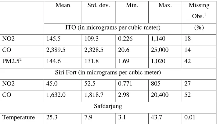
We measure pollution using data from monitoring stations at two different locations within the city, ITO and Siri Fort.14 Table 2 presents pollution statistics at each location, along with weather conditions at Safdarjung, Delhi. ITO has much higher pollution compared to Siri Fort: Average hourly NO2 and CO at ITO are 3.2 and 1.5 times their respective levels at Siri Fort. This is not surprising given that ITO is a major traffic intersection, while Siri Fort is a mainly residential area.
Ideally, we would have liked to know weather conditions specific to each location.
However, we only have hourly weather data for Safdarjung, which is fortunately located between ITO and Siri Fort. We use this as the best available proxy for weather conditions at each location. As the dynamics of pollution are likely to be different across the two locations, and also because they are at different distances from the various line expansions, we estimate impacts at each location separately.
At each location we estimate the impact of a particular metro extension using a time series of hourly pollutant data lying within a symmetric window around that extension’s opening date. We also ensure that there are no other extensions within this window. Thus, a window is characterized by a location l (ITO or Siri Fort) and an extension m. The RD approach is implemented by estimating the following OLS regression within each window:
, , , , , ,
0 1 2 3
l m= l m l m m l m l m l m
t t t t
y DM x P( )t u (1)
, l m
yt is pollutant level (in logs) in hour t, at location l, when studying the effect of extension m. DMtm is the discontinuity dummy for extension m: Within
14. In talking to experts at the CPCB, we were told that a monitoring station measures the quality of ambient air passing by it, and it is not possible to demarcate a precise catchment area for which the quality measure would apply. Given that the monitoring stations at ITO and Siri Fort are approximately 9 kilometers apart, we believe that they each measure air quality in two distinct geographies within the city. Some evidence for this is provided in table 2, which shows that average pollutant levels are very different across the two locations.
10
each window it takes the value 1 for all time periods after the extension date, and 0 for periods before it.15 xt, is the vector of covariates and includes controls for weather;16 for hour of the day,17 day of the week, and interactions between these two; and for public holidays and festivals such as Diwali.18 P(t) is a third-order polynomial in time and captures all smooth variations in pollutant levels. utl m, is the error term. The coefficient 1l m, measures the proportionate change in pollutant level at location l as a result of extension m. It is to be interpreted as the immediate localized (at location l) effect on pollution as a result of that particular extension.
Since we expect the traffic creation effect to be negligible in the short run, we do not expect 1,
l m to be positive. If there is a strong traffic diversion effect, 1,
l m will be negative, otherwise it will be insignificant.
Our identification strategy is similar to that used in Chen and Whalley (2012) (henceforth CW).19 CW look at the effect of the introduction of the Taipei Metro (TM) on air quality in Taipei City. While they use the discontinuity arising from the opening of the metro system, we exploit future discontinuities arising from various extensions of the network. Unlike CW, we do not use the first opening of the metro for two reasons. First, we do not have pollution data that
15. We exclude the 24-hour data pertaining to the day of the extension because we do not know the exact hour when the new line became operational.
16. Controls for weather include current and up to 4-hour lags of temperature, relative humidity, wind speed, and rainfall and quartics of both current and 1-hour lags of these weather variables.
17. Figures S1.1a through S1.1c in the supplementary appendix S1 show how the pollutants at ITO vary by hour of the day and by season. Once again we see that pollution is higher in winter compared to summer. Also, there is substantial intraday variation with peak levels reached between 8 pm and 2 am. Similar patterns are observed at Siri Fort. One plausible reason for why pollution peaks during these night hours could be a citywide ban on the entry and movement of heavy goods vehicles (mostly diesel powered trucks) between 6:00 am and 9:00 pm. The substantial intraday variation in pollution calls for inclusion of hour of the day fixed effects in order to improve the precision of our estimates. In most specifications season-fixed effects are not included because of short window lengths, typically nine weeks. Choice of window lengths is discussed later in this section.
18. Diwali is a Hindu festival that falls in winter, typically in October or November. It spreads over several days and is celebrated with an ostentatious bursting of firecrackers. It has been documented that air pollution in Delhi shoots up during and immediately following Diwali (CPCB 2012). It is therefore important to control for this source of pollution.
19. Before Chen and Whalley, Davis (2008) used similar identification to estimate the effect of driving restrictions on air pollution in Mexico City.
11
dates back to the time when the metro was introduced. Second, even if we had this data, it would be incorrect to use opening ridership discontinuity for Delhi. This is because there was an unprecedented jump in metro ridership when it was first opened, a large part of which was due to joy rides.20 These joy rides are expected to die out as the novelty of the metro fades away. By using discontinuities in ridership that occur a couple of years after the metro first started, we believe that to a large extent we avoid capturing effects arising from one time rides, and the impact that we measure is closer to the steady-state short-term effect.
One of the challenges that we faced in estimating equation (1) is the presence of segments of missing observations in each pollutant series. The last column of table 2 shows the share of missing observations.21 The best pollutant series is CO at ITO, for which 14 percent of observations are missing. PM2.5, which is only recorded at ITO, has 42 percent missing observations. For the RD strategy to be effective, there cannot be too many missing observations around the extension dates. Therefore, to begin with, we restrict our analysis to only those extensions for which there is a symmetric window of at least nine weeks around the date of extension, wherein missing observations in each included week do not exceed 20 percent of the potential observations.22 Then we look at other window lengths, and finally, for those pollutants with relatively good data, we analyze the entire series. In order to ensure correct inference in the presence of serial correlation in pollution, in all our specifications we use standard errors clustered at
20. “On the first day itself, about 1.2 million people turned up to experience this modern transport system. As the initial section was designed to handle only 0.2 million commuters, long queues of the eager commuters wishing a ride formed at all the six stations . . . Delhi Metro was forced to issue a public appeal in the newspapers asking commuters to defer joy rides as Metro would be there on a permanent basis” (DMRC 2008).
21. We were informed by a CPCB official that missing data could be due to many reasons: power cuts, instrument failure, software malfunction when transferring data to storage device, and disruption in telephone. According to the official, none of these reasons are systematically linked to high or low pollution episodes. Later on, in section IV, we examine whether there is evidence for a systematic pattern to missing observations.
22. At the hourly frequency, the number of potential observations in a week is 168 = 24*7. The 20-percent rule implies that each week in our estimation window has at least 134 = 0.8*168 observations.
12 one week.23
Plausibility of Identifying Assumption
Identification of the metro effect breaks down if we have not accounted for an event that has a discontinuous effect on air quality.24 One example is a citywide strike by private bus operators called on the same day as the extension of the metro. If this happens it would be impossible to disentangle the effect of the metro from that of the strike. We have studied the chronology of events in the city and do not find occurrences of such events on any of the extension dates. Here we discuss some of the other likely threats to identification.25
Government policies aimed at reducing pollution may have an abrupt impact. One such policy, implemented only in Delhi, was the mass conversion of diesel fueled buses to compressed natural gas (CNG). However, this happened in 2001, well before our study period began, and is therefore not problematic. In 2005, Delhi moved from Bharat Stage-II to the stricter Bharat Stage-III emission standards. Although this regulatory change was implemented in the middle of our study period, it is unlikely to have led to a sudden change in pollution. This is because the improved norms are only applicable for vehicles manufactured after the new standards were adopted. Given that new vehicle registrations happen uniformly over time, adoption of stricter emission standards should not lead to a sudden drop in vehicular emissions.26 We do not know of any other regulatory
23. Although, both Chen and Whalley (2012) and Davis (2008) use standard errors clustered at five weeks, we cluster at one week. This is because our analysis is based on shorter windows of five and nine weeks (due to missing data), while they use two-year horizons. Also, for all pollutants in our data, the auto correlation in daily average pollutant level is less than 0.5 beyond seven days. Clustering at one week should therefore be sufficient.
Nonetheless, we re-estimated tables 4 and 5 by clustering at two weeks and found similar results.
24. An event that has a gradual effect on pollution will be captured by the time polynomial P(t) and therefore does not impede our analysis.
25. For them to be problematic, the discontinuous effects do not have to necessarily happen on the extension date.
Discontinuous effects arising anywhere within our short windows would be problematic for estimating the correct causal effect of the metro extension.
26. Emission standards in India are adopted in a phased manner with stricter norms first being implemented in major cities, including in Delhi, and then extended to the rest of the country after a few years. Given that inter-state freight that plies through Delhi continues to follow the more relaxed emission standards, the impact of Bharat Stage-III
13
change implemented between 2004 and 2006 that may have had a discontinuous effect on pollution.
Another concern could be that construction activity undertaken to build the new rail lines may have added to localized pollution in the period preceding the metro extension and this would then over-estimate the DM effect. On speaking to officials from the DMRC we were told that such construction activity is typically completed fifteen to thirty days prior to the opening of a new line so as to conduct trial runs to ensure safety of passengers. Therefore, at least for the shorter window lengths, we do not expect this issue to be a problem. Another worry could be that metro officials choose the extension dates in a systematic manner to coincide with either high- or low-pollution days. We think that this is highly unlikely. Given the public enthusiasm for the metro and the recognition of economies of scale in its operation, the DMRC has always been eager to open a new line once it had met all safety requirements.
Finally, Delhi is characterized by a multitude of pollution sources.
According to Guttikunda and Calorie (2012), domestic sources, such as burning of biofuel for cooking and heating, use of diesel generator sets, waste burning, and construction, together account for 20, 19, and 26 percent of NOx, CO, and PM2.5, respectively. These sources tend to be sporadic and sometimes mobile, and it is possible that we have not accounted for all of them. In the results section we talk about what definitive conclusions may be drawn in spite of this threat to identification.
IIIDATA SOURCES
All the data used in this study are from secondary sources. Data on pollutants were obtained from the Central Pollution Control Board (CPCB), which
within Delhi is dampened.
14
collects it as part of the National Air Quality Monitoring Program (NAMP). We use hourly pollution data recorded at two monitoring stations in the city, namely at ITO and at Siri Fort.27 Both are immobile stations that operate on electricity. They provide comparable data as they were bought from the same manufacturer and followed the same monitoring protocol throughout our study period. Hourly data on weather conditions at Safdarjung, Delhi, were obtained from The National Data Center of the India Meteorological Department. Our choice of study period (2004–
2006) was dictated by the overlapping period for which we had both pollution and weather data. The Delhi Metro Rail Corporation (DMRC) provided us with data on metro ridership.
IVRESULTS
Before presenting the impact estimates, we investigate whether the data validate a sudden increase in metro ridership at the time of each extension.
Ridership Discontinuities
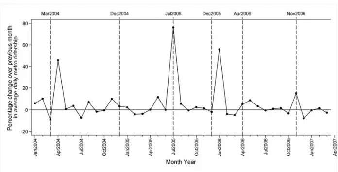
For each month, figure 3 shows the percentage change in average daily ridership on the DM over the previous month.28 The exact magnitudes of change are given in the last column of table 1. Except for the introduction of the Yellow Line and the first extension of the Blue Line, the figure shows a significant rise in average daily ridership for the month (or for the following month)29 of each extension.
27. Under the NAMP there is one other monitoring station located at the Delhi College of Engineering (DCE) in north Delhi. We do not use data from this station because our identifying assumption is unlikely to hold at this location. Compared to ITO and Siri Fort there are many more erratic sources of pollution at DCE. This is because, (a) it is surrounded by Badli, a major industrial township; (b) all along its periphery there are other small scale industrial production units; (c) during our study period the college building itself was undergoing repair and renovation; and (d) DCE is in a mainly rural part of Delhi where sporadic burning of biomass and wood is widespread.
28. Actual daily ridership, instead of average daily ridership in a month, would have been ideal in order to check the sudden increase in ridership at each extension date. However, this data was not available for our study period.
29. For the second extension of the Red Line and the first extension of the Blue Line, we see the surge in ridership in the month following the one in which the extension took place. This is because these extensions were introduced on the last day of the month, and one would therefore expect average ridership to increase only in the following month.
15
The absence of a significant rise in ridership for the introduction of the Yellow Line (3 percent increase) may be attributed to the fact that it was the first segment of the north-south corridor and also a short segment (3 additional stations) that connected the university to the existing Red Line at a time when the university was closed for the holiday season. Further, besides the university station, the two other stations on this segment are relatively rich neighborhoods where many people may continue to prefer private over public transportation. For the first extension of the Blue Line, the insignificant rise in ridership (5 percent increase) may be attributed to the relatively lower population density in south-west Delhi where the extension took place.30 Given the necessity of observing a large surge in ridership in order to identify the DM effect, we exclude these two extensions from our analysis.
The largest jump in ridership is seen for the first extension of the Yellow Line (76 percent increase), which connects areas having a high population density (North-East and Central districts) to the hub of government offices in Central Secretariat. A large surge in ridership is also seen for the introduction of the Blue Line (56 percent increase) which is the longest extension among all the extensions considered here.
Given this ridership pattern we expect to see larger effects for the first extension of the Yellow Line and the introduction of the Blue Line. We also expect larger effects at ITO than at Siri Fort because of its relative proximity to the line expansions and also because it is a major traffic intersection whereas Siri Fort is mainly residential.
Impact Estimates: Short Windows
In order to estimate equation (1) using fairly good quality data with fewer
30. Of the nine districts of Delhi, the South-West district had the lowest population density of 4,179 persons per square kilometer in 2001. The North-East district had the highest: 29,468 persons per square kilometer (Govt. of NCT of Delhi 2008a).
16
missing values, table 3 shows the maximum window length (in weeks) around each extension on applying the at-most-20-percent-missing-data criteria for each included week and also subjecting the selection to a minimum window length of five weeks. As an example, if we restrict ourselves to good quality data, we are able to examine the effect of the second extension of the Blue Line on NO2 at ITO using a maximum window length of only thirteen weeks. Of the four extensions characterized by a significant increase in ridership, we are unable to examine the effects of the second extension of the Red Line because of lots of missing observations around its opening date.
For all extensions with at least nine weeks of good quality data,31 figures S1.2a through S1.2h in the supplementary appendix S1, try to visually examine whether there is a break in a pollutant series at the extension date using a nine- week window around the date.32 These plots suggest that there is a drop in pollutant level at the time of each extension, and in some cases this drop is large.
Next, we estimate equation (1) to arrive at quantitative estimates.
Table 4 shows the results from an estimation of equation (1) using a nine- week symmetric window of good quality data around each extension date. For each location, it shows the percentage change in the pollutant level that may be attributed to a specific metro extension.33 Contrary to our expectations, the first extension of the Yellow Line did not lead to a statistically significant drop in the level of NO2 at ITO, but as expected it resulted in a huge drop of 69 percent in CO
31. For PM2.5 at ITO we only have a seven-week window of good quality data, and therefore we look at this shorter window of seven weeks for it.
32. The scatter points are daily averages of residuals obtained from a regression of (log) hourly pollutant on all the right-hand side variables in equation (1) except the extension discontinuity, DMtm, and the time polynomial, P(t).
The overlaid curve depicts the fitted residuals from a regression of the scatter points on the extension discontinuity and a third order time polynomial.
33. When calculating the percentage change we apply the correction suggested by Kennedy (1981) in the context of interpreting the coefficient on a dummy variable in a semi logarithmic equation.
17
at ITO. The introduction of the Blue Line resulted in a 31 percent decrease in the level of NO2 at ITO. Its effect on CO at ITO could not be analyzed because of missing data. We had expected the second extension of the Blue Line to lead to smaller declines, and we find that it did not lead to statistically significant reductions in any of the three pollutants. Turning to the effects at Siri Fort, we were only able to examine the second extension of the Blue Line. Our analysis shows that just as for ITO, this extension did not lead to a statistically significant decrease in either NO2 or CO at Siri Fort. It is to be noted that even where an effect is not statistically significant, its sign is always negative and in some cases the magnitude is not insignificant.
Table 5 shows the impacts using a shorter window of five weeks. Compared to the nine-week window, although the magnitude of impact of the first extension of the Yellow Line on NO2 at ITO is larger, it is still not statistically significant.
The effect on CO at ITO for this extension has increased to 78 percent. Also for the introduction of the Blue Line, the effect on NO2 at ITO has increased to 55 percent.
Restricting to a shorter window enables us to study the effects of this extension on CO and on PM2.5: at ITO it led to a decrease of 56 and 53 percent, respectively.
The results for the second extension of the Blue Line at ITO and Siri Fort are similar to those seen in table 4 and continue to remain statistically insignificant.
As seen in table 3 there are segments of good quality data that span longer than nine weeks. In table 6 we extend the window beyond nine weeks whenever the data permit us to do so. In most cases there is a decrease in magnitude of impact, and none of the effects are significant now. We provide two plausible explanations for the transitory nature of our impact estimates.
One explanation is that some of the sporadic and mobile sources of pollution that characterize Delhi’s pollution inventory get captured when we extend the
18
window, and this masks the impacts for longer time periods. Admittedly, this may also happen for shorter windows, and it could even explain the very large magnitudes for some of the estimates seen in tables 4 and 5.34 As discussed in section II, these sporadic and mobile sources of pollution pose a threat to our identification strategy. However, the fact that when we look at shorter time periods we consistently get negative estimates (in table 4 all estimates are negative, and in table 5, all except one (which is close to zero), are negative), makes us believe that some of the larger extensions did reduce specific transportation source pollutants even if the exact magnitudes of reduction may not be those reported in tables 4 and 5.
Another explanation for the disappearance of effects in table 6 could be that the traffic diversion effects are indeed transitory and over longer time horizons the DM has no impact on pollution. Duranton and Turner (2011) provide evidence in support of this argument. They find that in cities in the United States, increase in road-building and provision of public transport have no impact on vehicle- kilometers-traveled. They reason that reduced congestion on roads, experienced soon after new roads are built, has a feedback effect that induces existing residents to drive more. If this is true for Delhi, then it is possible that soon after the larger extensions were initiated, the DM diverted private traffic which lowered pollution (as seen in tables 4 and 5 using shorter windows) and also reduced road congestion. These reductions in turn incentivized the remaining drivers to drive more, and may have also added some new drivers, thus wiping out the initial
34. Additionally, it could also explain some of the inconsistencies in our impact estimates. As pointed out earlier in this section, we had expected the first extension of the Yellow Line to lead to a reduction in both NO2 and CO.
However, while we see a substantial reduction in CO, the effect on NO2 is not statistically significant (see tables 4 and 5). There is also a discrepancy across extensions in the sense that while the magnitude of effects on NO2 and CO at ITO are comparable for the introduction of the Blue Line, for the first extension of the Yellow Line these are quite disproportionate (see table 5).
19
effects on pollution (as seen in table 6) and on road congestion. This explanation is along the lines of the traffic creation effect discussed earlier. Unfortunately, our data and empirical strategy do not allow us to discern with surety which of these explanations is true. However, our subsequent analysis using data for the entire study period suggests that the effects may not be transitory.
Robustness Checks
Here we present some robustness checks for the results seen in table 4. We also present results from a new specification that uses all the data for our study period, ignoring the fact that there are missing observations. For reasons stated below, this is our preferred specification.
Varying the Order of the Time Polynomial: Following CW, we have used a third order time polynomial. However, in specifications similar to ours, Davis (2008) uses a seventh order polynomial. In order to check that our main results are robust to the choice of polynomial order, we ran the regressions in table 4 using a fourth through seventh order polynomial and found similar estimates. The results for the fourth and the seventh order specifications are shown in tables S1.2a and S1.2b in the supplementary appendix S1.35
Accounting for Persistence in Pollution: Next we examine whether controlling for lagged pollution alters the estimated impacts. We estimate the equation shown below (l, m superscripts have been suppressed):
0 1 2 3 1 1 2 2 3 3 4 4
t = t t t t t t t
y DM x P( )t y y y y e
The results are shown in tables S1.3a and S1.3b in the supplementary appendix S1.
As expected, when we account for persistence, the instantaneous impacts are lower.36 The two instances in table 4 where we had seen significant drops in
35. We also tried interacting the time polynomial with the discontinuity dummy, DMtm. We do not report these results as, in all cases, the discontinuity dummy drops out due to multicollinearity in our dataset.
36. The instantaneous impact is 1, and the cumulative effect is calculated by iteratively substituting for y in the
20
pollution continue to remain significant, although the magnitude of the cumulative effects is lower.
Artificial Discontinuities: For NO2 and CO, we implemented the standard placebo test of using data only from the pretreatment period (before the extension is made) and introducing artificial discontinuities within this period. In some cases we did find significant effects. In the same vein, we estimated equation (1) using the introduction of the Yellow Line, which is characterized by an insignificant jump in ridership (see earlier discussion under “Ridership Discontinuities”). For this expansion, we had expected to find insignificant effects, but instead we found significant declines in both NO2 and CO at Siri Fort. These perverse results could be due to sporadic and mobile sources of pollution in Delhi. While we admit that this is a potential threat to identification, the fact that we consistently get negative effects for all discontinuities in tables 4 and 5 and that, in most cases, these effects are larger when we reduce the time window, provides strong support that DM did reduce pollution. Below, we provide additional evidence to support this claim.
Effects on Nontransportation Source Pollutants: Our conjecture is that traffic diversion is the main mechanism through which the DM affects pollution in the short run. We can test this by looking at the effects of various extensions on the two nontransportation source pollutants, namely, sulphur dioxide, SO2, and ozone,
3.
O If our hypothesis is true, then, we should not find any effects on these pollutants. In fact, CW use this as a robustness check for their results. We first explain why using O3 for such a robustness check is invalid in our context. Then, we implement the check using SO2 and discuss the results.
Formation of O3 crucially depends on the ratio of volatile organic
equation shown. The cumulative effect is then given by,
2 3 4 2 2
1 1 1 1 1 2 1 2 1 3 2 2 3 4 1
[1 3( ) 2 2 ] .
21
compounds (VOC) to NOx (Sillman, 1999). The relationship between O3, VOC, and NOx is nonlinear, and given that there is evidence that NO2 (and perhaps, VOC, as well), was impacted by the DM, ex-ante it is not possible to know whether or not the DM would affect O3, and if it does, in what direction. Hence, we do not use O3.
Table S1.4 in supplementary appendix S1 presents the results when we estimate equation (1) using SO2 at ITO as the dependent variable. We examine impacts for the first extension of the Yellow Line and for the introduction of the Blue Line; the two discontinuities for which we found significant declines in transportation source pollutants in table 4.37 We had expected to see no impact but table S1.4 shows large positive effects for both extensions. This may be explained by the presence of three coal based power plants within the National Capital Region of Delhi (marked as triangles in figure 2) during our study period.
According to Gurjar et al., 2004, and Guttikunda and Calorie, 2012, 68 and 55 percent, respectively, of SO2 in Delhi is generated by these power plants. Figure S1.3 in the supplementary appendix S1 shows wide variation in the monthly power production of these plants. More importantly, it shows that monthly output was either high or rising when the two extensions were made. Since SO2 emissions are strongly correlated with power produced, there will be corresponding variations in SO2. Thus, it is possible that it is the coal plants that are behind the significant impacts seen in table S1.4. In any case, that the two metro expansions were accompanied by an increase in SO2 increases the credibility that these expansions led to reductions in some transportations source pollutants (as seen in table 4).
Missing Data Patterns: Since our analysis so far has been based on examining particular segments of good quality pollutant data, it is important that
37. In this exercise usingSO2, for both discontinuities, we use a nine week window and once again adopt the criteria of at most 20 percent missing observations for each included week.
22
observations should not be missing systematically. For each pollutant, table S1.5 in supplementary appendix S1, provides time series of share of missing observations in each month between 2004 and 2006. Eye balling the data does not suggest a pattern to missing observations. We examine this more thoroughly in two ways.
First we examine whether there is any association between data being missing and the timing of metro expansions. To do this we use data for our entire study period, 2004–2006, and estimate equation (1) by replacing the outcome variable with an indicator variable for whether the pollutant measure is missing. In this specification we include all six discontinuity dummies (representing the six metro expansions undertaken in this period), and also include season fixed effects.
Results are presented in tables S1.6a and S1.6b for ITO and Siri Fort, respectively, in supplementary appendix S1. At ITO, for NO2 and PM2.5 there is some evidence that observations are less likely to be missing in summer. However, given that for each pollutant some extensions are positive, some negative, and some insignificant, we conclude that the extensions by themselves are not systematically associated with the pollutant measure being missing.
Next we investigate whether observations are more likely to be missing on either high or low pollution days. This is done using the entire series for CO and PM2.5 at ITO. The last column of table 2 shows that CO at ITO has 14 percent missing observations, while the corresponding figure for PM2.5 is 42 percent. Given these shares of missing observations, we use a specification similar to equation (1), wherein missing status for PM2.5 is regressed on whether or not CO is above the CPCB prescribed limit of 2000g m/ 3 (proxy for high pollution). Other right hand side variables are the same except that we drop the discontinuity dummies and the time polynomial, and once again include season fixed effects. The results are shown in appendix table S1.7 in supplementary appendix S1. The coefficient on