The Day-of-the-Week Effect Revisited: An Alternative Testing Approach

IHS Economics Series Working Paper 127

November 2002

The Day-of-the-Week Effect Revisited: An Alternative Testing Approach

Raimund Alt

Ines Fortin

Simon Weinberger

Impressum Author(s):

Raimund Alt, Ines Fortin, Simon Weinberger Title:

The Day-of-the-Week Effect Revisited: An Alternative Testing Approach ISSN: Unspecified

2002 Institut für Höhere Studien - Institute for Advanced Studies (IHS) Josefstädter Straße 39, A-1080 Wien

E-Mail: o ce@ihs.ac.atffi Web: ww w .ihs.ac. a t

All IHS Working Papers are available online: http://irihs. ihs. ac.at/view/ihs_series/

This paper is available for download without charge at:

https://irihs.ihs.ac.at/id/eprint/1464/

The Day-of-the-Week Effect Revisited: An Alternative Testing Approach

Raimund Alt, Ines Fortin, Simon Weinberger

127

Reihe Ökonomie

Economics Series

127 Reihe Ökonomie Economics Series

The Day-of-the-Week Effect Revisited: An Alternative Testing Approach

Raimund Alt, Ines Fortin, Simon Weinberger November 2002

Institut für Höhere Studien (IHS), Wien

Institute for Advanced Studies, Vienna

Contact:

Raimund Alt

Department of Economics and Finance Institute for Advanced Studies

Stumpergasse 56, A-1060 Vienna, Austria (: +43/1/599 91-159

email: alt@ihs.ac.at

Ines Fortin

Department of Economics and Finance Institute for Advanced Studies

Stumpergasse 56, A-1060 Vienna, Austria (: +43/1/599 91-165

email: fortin@ihs.ac.at

Simon Weinberger

email: simonweinberger@hotmail.com

Founded in 1963 by two prominent Austrians living in exile – the sociologist Paul F. Lazarsfeld and the economist Oskar Morgenstern – with the financial support from the Ford Foundation, the Austrian Federal Ministry of Education and the City of Vienna, the Institute for Advanced Studies (IHS) is the first institution for postgraduate education and research in economics and the social sciences in Austria.

The Economics Series presents research done at the Department of Econom ics and Finance and aims to share “work in progress” in a timely way before formal publication. As usual, authors bear full responsibility for the content of their contributions.

Das Institut für Höhere Studien (IHS) wurde im Jahr 1963 von zwei prominenten Exilösterreichern – dem Soziologen Paul F. Lazarsfeld und dem Ökonomen Oskar Morgenstern – mit Hilfe der Ford- Stiftung, des Österreichischen Bundesministeriums für Unterricht und der Stadt Wien gegründet und ist somit die erste nachuniversitäre Lehr- und Forschungsstätte für die Sozial- und Wirtschafts - wissenschaften in Österreich. Die Reihe Ökonomie bietet Einblick in die Forschungsarbeit der Abteilung für Ökonomie und Finanzwirtschaft und verfolgt das Ziel, abteilungsinterne Diskussionsbeiträge einer breiteren fachinternen Öffentlichkeit zugänglich zu machen. Die inhaltliche Verantwortung für die veröffentlichten Beiträge liegt bei den Autoren und Autorinnen.

Abstract

This paper questions traditional approaches for testing the day-of-the-week effect on stock returns. We propose an alternative approach based on the closure test principle introduced by Marcus, Peritz and Gabriel (1976), which has become very popular in Biometrics and Medical Statistics. We test all pairwise comparisons of daily expected stock returns, while the probability of committing any type I error is always kept smaller than or equal to some prespecified level a for each combination of true null hypotheses. We confirm day-of-the- week effects for the S&P 500, the FTSE 30 and the DAX 30 found in earlier studies, but find no evidence for the 1990's.

Keywords

Day-of-the-week effect, multiple hypotheses testing, multiple comparisons, closed test procedures, multiple level a test

JEL Classifications

C12, C20, G14

Contents

1 Introduction 1

2 Traditional Testing Approaches 3

3 Closed Test Procedures – An Alternative Approach 6

4 Data 11

5 Results 14

6 Conclusion 26

References 28

1 Introduction

In recent decades the testing for market anomalies in stock returns has become an active …eld of research in empirical …nance. Some anomalies have attracted much attention not only in academic journals but also in the

…nancial press. Among the more well-known anomalies are the size e¤ect, the January e¤ect and the day-of-the-week e¤ect (Monday e¤ect).

Since Cross (1973) observed negative returns on Mondays for the US stock market, numerous studies have been devoted to the examination of day-of- the-week e¤ects, in particular irregularities a¢liated with Monday returns (see e.g. French (1980)). Negative Monday returns were found to be robust over time and di¤erent markets early after (see Ja¤e and Wester…eld (1985) and Keim and Stambaugh (1984)). Also more recent studies, examining data until the early 1990’s document the existence of a day-of-the-week e¤ect in major markets (see e.g. Dubois and Louvet (1996)). Meanwhile various methodological issues related among others to time series properties of stock returns have been addressed (see e.g Connolly (1991) and Chang, Pinegar and Ravichandran (1993)).

Though testing for market anomalies often involves the use of several tests, it is a matter of fact that empirical studies often do not appropriately ac- count for the multiplicity e¤ect. This may lead to an in‡ated occurrence of multiple type I errors producing spurious signi…cance with regard to the test results. To overcome this problem we propose an alternative approach for testing the day-of-the-week e¤ect, which di¤ers from traditional approaches in two respects. First, we test all pairwise comparisons of daily expected stock returns. Second, the null hypotheses of interest are tested in such a way, that the multiple level ® is controlled, i.e. the probability of commit-

ting any type I error is always smaller than or equal to the given level ®.

The latter property, which holds for each combination of true null hypothe- ses, is guaranteed by the application of the so-called closure test principle introduced by Marcus, Peritz and Gabriel (1976).

Closure tests have become very popular in Biometrics and Medical Statis- tics, which is due to the fact that they are often more powerful than classic multiple test procedures (see Pigeot (2000) for a recent survey). Aside from a few exceptions like Neusser (1991) or Madlener and Alt (1996), closed test procedures, as they are also called, seem to be quite unknown in the economics and …nancial literature. In particular, Savin (1984) did not men- tion them in his survey, although these procedures were already used in the 1970’s.

We are not the …rst to address the problem of controlling type I error proba- bilities in empirical studies on market anomalies. Recently, Greenstone and Oyer (2000) have suggested the use of the Bonferroni procedure, a simple but rather conservative method. Another approach was suggested by Sulli- van, Timmermann and White (2001), who use a computationally intensive bootstrapping procedure to account for the multiplicity e¤ect in studies on calendar anomalies. In some sense our proposal can be seen as a middle- of-the-road approach. On the one hand, closed test procedures are based on a relatively simple construction involving level ®tests for all intersection hypotheses. On the other hand, the resulting multi-step or stepwise proce- dures are often more powerful than classic single-step procedures, like for example, the Bonferroni procedure.

The paper is organized as follows. Section 2 discusses traditional approaches for testing the day-of-the-week e¤ect. Section 3 explains the closure test

principle and its implementation for the problem at hand. Section 4 provides a description of the used data set. Section 5 presents the results of the closed test procedure applied to daily returns of the S&P 500, the FTSE 30 and the DAX 30 for the period 1971-2001 as well as three subperiods. Section 6 concludes the paper.

2 Traditional Testing Approaches

The testing for day-of-the-week e¤ects on stock returns usually involves re- gression models with dummy variables. Meanwhile there are numerous ex- tensions, but for convenience let us restrict ourselves to the following basic model set-up. Let R_is denote the return on day iduring the weeks. Then R_is can be written as

R_is=E(R_is) +"_is, (1)

whereE(Ris)is the expected value ofRis and"is is the corresponding error term. Usually it is assumed that the expected return on day i is constant over all weeks of the observation period. In this case (1) becomes

Ris=°_i+"is, (2)

where °_i ´E(R_is).

The above equations can be formulated jointly as a regression equation with dummy variables:

R_t =°₁d_1t+°₂d_2t+°₃d_3t+°₄d_4t+°₅d_5t+"_t. (3)

Rt is now the return on any day of the week, the dummy variables dit, 1 ·i·5;indicate the day of the week, on which the returnR_twas observed, and"t is the error term,1·t·T,T being the number of all observations.

In particular, d_1t = 1 indicates that the return was observed on a Monday, d2t = 1indicates a Tuesday return and so on. Whenever dit= 1 for some i, then d_{j t}= 0 for all j6=i.

The usual approach is then to test the global null hypothesis,

H0: °₁ =°₂=°₃ =°₄ =°₅,

that all expected daily returns are equal. If H₀ is not rejected at a given level®, then one concludes that there is no evidence that the expected daily returns are di¤erent. Otherwise, in case that H₀ is rejected, it is common practice, to look at the values of the t-statistics for the single regression coe¢cients, assuming °_i = 0. In other words, the additional null hypotheses

H_i: °_i = 0 1·i·5

are tested, though this is often done in a more implicit way.

An alternative formulation of (2) is

R_is = 8>

<

>:

±₁+"_1s if i= 1

±₁+±_i+"_is if2 ·i·5

where ±₁ ´°₁ has the same meaning as in (2), while the di¤erences ±_i ´

°_i¡°₁ measure the expected excess return of some day i of the week over a speci…c other day (in this case Monday). The regression equation then

looks as follows:

Rt=±1+±2d2t+±3d3t+±4d4t+±5d5t+"t.

The global null hypothesis that all expected daily returns are equal can be formulated as:

H₀: ±₂ =±₃ =±₄ =±₅ = 0.

If H₀ is not rejected at level®, then one concludes that there is no evidence that the expected excess returns are di¤erent from zero. Otherwise, if H0 is rejected, the null hypotheses

H_i: ±_i = 0 2·i·5

are tested as well. The rejection of, sayH_i, would indicate that there is some evidence that the expected returns between dayiand Monday, respectively, are di¤erent.

We think that both testing approaches su¤er from some serious drawbacks.

With regard to the …rst approach, the testing of the null hypotheses Hi:

°_i= 0,1·i·5, is questionable, to say the least. If there is some evidence that the expected daily returns are not equal, what is the logic behind the next step to test the null hypotheses that each expected daily return is equal to zero? One of the problems of the second approach is that it is obviously biased towards Monday, in the sense that it is only the expected Monday return which is compared to the expected return of each other day.

In particular, if H2 is tested and not rejected, there is still a chance for Monday to be di¤erent, namely when H₃ is tested, and so on. But there is

another problem inherent in both approaches. Each of the described testing strategies requires the testing of several null hypotheses. If this is done in the traditional way by using tests, each having a signi…cance level of 5%, then this may result in spurious signi…cance in the employed tests. The reason for this is that the type I error probability for each testing approach may be much larger than 5%.

To overcome these problems we suggest an alternative approach, which dif- fers from the traditional approaches in two ways. First, if the global null hypothesisH₀ is rejected, we test a new set of null hypotheses, namely the multiple comparisons H_ij: °_i = °_j, for all 1 · i < j ·5, resulting in an unbiased, symmetric test design. Second, the null hypotheses are tested in such a way, that the probability of committing any type I error is always kept smaller than or equal to some given level ®, for each combination of true null hypotheses. The testing procedure is based on the so-called closure test principle, which we describe in the following section.

3 Closed Test Procedures - An Alternative Ap- proach

Closed test procedures, which were introduced by Marcus, Peritz and Gabriel (1976), belong to the class of multiple level® tests. A multiple level® test is a test procedure with the property that the probability of committing any type I error is always smaller than or equal to the given level ®, for each combination of true null hypotheses. A simple example for a multiple level ® test is the well-known Bonferroni procedure, where each of the null hypothesesH₀₁; :::; H_0nis tested at the level®=n. The multiple level® prop-

erty of the Bonferroni procedure can be shown by applying the Bonferroni inequality to the type I error probability

P Ã[

i2I

fH_0i is rejectedg

!

· X

i2I

P (H0i is rejected)

= jIj ¢® n

· ®

where I is the index set of the true null hypotheses and jIj is the number of elements in I. A major disadvantage of the Bonferroni procedure is the fact that the type I error probability can sometimes become very small compared to the given level ®, for example, if the number jIj of true null hypotheses is small. A recent application of the Bonferroni procedure in

…nance is due to Greenstone and Oyer (2000), who tested various calendar based anomalies. Meanwhile, many classic single-step procedures have been replaced by closed test procedures, since the latter are usually considered to be more powerful. There are some empirical studies, e.g. Chow and Denning (1993) or Huber (1997), where the use of the Sidak inequality results in slightly larger signi…cance levels for the single tests compared with those of the Bonferroni procedure. For practical purposes, however, the additional gain in power is negligible.

The application of closed test procedures is based on two assumptions. First, the set H=fH₀₁; :::; H_0ng of interesting null hypotheses has to be closed under intersection, i.e. it is required thatH0i\H0j 2 Hfor any two indices i 6= j. Second, there should be available a multiple test procedure © = (Á₁; :::; Á_n), where each testÁ_i is a level ® test for the null hypothesis H_0i;

1 ·i·n. Given these two assumptions one can apply the so-called ’closure test principle’, resulting in a test procedure which keeps the multiple level

®, i.e. the probability of committing any type I error is always less than or equal to the given level®; for each combination of true null hypotheses.

The closure principle works as follows. One de…nes another test procedure ª = (Ã₁; :::; Ã_n), which combines the results of the testsÁ₁; :::; Á_n in such a way that the test procedure ª is a multiple level ® test. Each test Ã_i; i= 1 ·i·n; is de…ned by the following rule:

RejectH_0i, if each subhypothesisH_0j ½H_0i is rejected by its level® test Á_j,

where a subhypothesis ofH_0i is any element inHwhich is contained inH_0i, includingH_0i itself. Marcus, Peritz and Gabriel (1976) have shown that the test procedureª = ( Ã₁; :::; Ã_n) keeps the multiple level®.

With regard to regression equation (3) we want to test all pairwise compar- isons

Hij: °_i =°_j 1·i < j·5, provided that the global null hypothesis

H₀: °₁ =°₂=°₃ =°₄ =°₅

has been rejected.

In order to apply the closure test principle we have to consider the two

assumptions described above. Obviously the set of null hypotheses

H=fH0; H12; H13;H14; H15; H23; H24; H25; H34; H35; H45g

we are interested in, is not closed under intersection, e.g. the intersection H₁₂\H₁₃ = f°₁ =°₂ =°₃g is not an element of H. Therefore, in order to get a closed set H^¤ of null hypotheses, we have to add as auxiliary hy- potheses all possible intersections of the sets in H. Table 1 lists all pairwise comparisons Hij :°_i = °_j;1 · i < j · 5; together with all possible inter- sections.

Since we are interested in testing all pairwise comparisons H_ij: °_i = °_j, 1 ·i < j·5, the closure principle requires that all subhypotheses of each comparison have to be tested by their corresponding level ® tests. It will turn out, however, that this is not always necessary.

If, for example,H₀ is not rejected at level®, the procedure stops and none of the null hypotheses will be rejected. This is so, becauseH0is a subhypothesis of each hypothesis inH^¤ and, therefore, given the closure test rule described above, no null hypothesis can be rejected by the tests Ã₁; :::; Ã_n. On the other hand, ifH₀ is rejected at level®, one has to consider the subhypotheses of each comparison H_ij: °_i =°_j. Whenever a subhypothesis ofH_ij cannot be rejected at level ®, this immediately implies thatH_ij cannot be rejected by the closure test.

Hij H_ijk H_{ij kl} H12345 =H0

°₁ =°₂ °₁ =°₂ =°₃ °₁=°₂=°₃ =°₄ °₁ =°₂ =°₃=°₄=°₅

°₁ =°₃ °₁ =°₂ =°₄ °₁=°₂=°₃ =°₅

°₁ =°₄ °₁ =°₂ =°₅ °₁=°₂=°₄ =°₅

°₁ =°₅ °₁ =°₃ =°₄ °₁=°₃=°₄ =°₅

°₂ =°₃ °₁ =°₃ =°₅ °₂=°₃=°₄ =°₅

°₂ =°₄ °₁ =°₄ =°₅

°₂ =°₅ °₂ =°₃ =°₄

°₃ =°₄ °₂ =°₃ =°₅

°₃ =°₅ °₂ =°₄ =°₅

°₄ =°₅ °₃ =°₄ =°₅

H_ij;kl H_{ij k;lm}

°₁ =°₂ ^°₃=°₄ °₁=°₂ =°₃ ^°₄ =°₅

°₁ =°₂ ^°₃=°₅ °₁=°₂ =°₄ ^°₃ =°₅

°₁ =°₂ ^°₄=°₅ °₁=°₂ =°₅ ^°₃ =°₄

°₁ =°₃ ^°₂=°₄ °₁=°₃ =°₄ ^°₂ =°₅

°₁ =°₃ ^°₂=°₅ °₁=°₃ =°₅ ^°₂ =°₄

°₁ =°₃ ^°₄=°₅ °₁=°₄ =°₅ ^°₂ =°₃

°₁ =°₄ ^°₂=°₃ °₂=°₃ =°₄ ^°₁ =°₅

°₁ =°₄ ^°₂=°₅ °₂=°₃ =°₅ ^°₁ =°₄

°₁ =°₄ ^°₃=°₅ °₂=°₄ =°₅ ^°₁ =°₃

°₁ =°₅ ^°₂=°₃ °₃=°₄ =°₅ ^°₁ =°₂

°₁ =°₅ ^°₂=°₄

°₁ =°₅ ^°₃=°₄

°₂ =°₃ ^°₄=°₅

°₂ =°₄ ^°₃=°₅

°₂ =°₅ ^°₃=°₄

Table 1: Pairwise Comparisons and All Intersection Hypotheses.

4 Data

In order to empirically investigate the day-of-the-week e¤ect we consider three major stock markets, the US (S&P 500), the UK (FTSE 30) and Germany (DAX 30). We extract daily closing levels of the selected indices from Thomson Financial/Datastream from January 1, 1971 to December 31, 2001 and compute daily returns on the indices as logarithmic returns

Rt = ln( P_t P_t¡1);

where P_t are daily closing prices. To each return observation we assign the corresponding day of the week and generate a set of dummy variables indicating that day. As Monday return e.g. we consider the change from Friday close to Monday close. We exclude days, when markets are closed due to national holidays. So if Wednesday, for example, is a national holiday, the Thursday return is computed from the Tuesday to the Thursday close, resulting in a total of four observations for that particular week. In contrast to the S&P 500 and the FTSE 30, the DAX 30 is a performance index, i.e. it explicitly accounts for dividend payments. As we are not aware of any empirical evidence that dividend payments across all shares contained in the index occur primarily on any particular day of the week, the impact of single dividends on index returns should be of minor importance for our investigation.

To get a more detailed picture of our results we divide the total sample period into three subsamples, subperiod 1 (January 1, 1971 to December 31, 1980), subperiod 2 (January 1, 1981 to December 31, 1990), and subperiod 3 (January 1, 1991 to December 31, 2001). All tests we employ will thus be

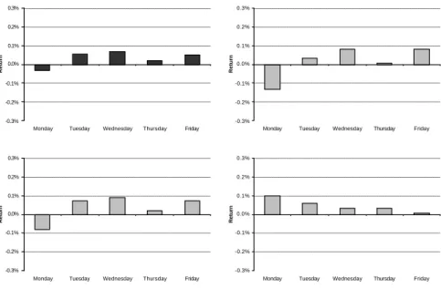
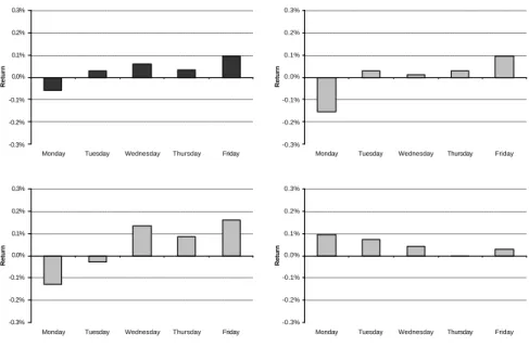
carried out …rst for the total period ranging from 1971 to 2001, and second for each of the three subperiods. Figures 1 to 3 plot the average rate of return per day of the week for the S&P 500, the FTSE 30 and the DAX 30.

The …rst graph (black coloured) shows the average rates of return of the total period, the remaining graphs (grey coloured) show the corresponding numbers for the three subperiods.

Considering the total period, we observe a negative average Monday return in each of the markets, whereas all other average returns are positive, except for the FTSE 30 Thursday returns. If we take a closer look at the subsam- ple returns, though, the empirical pattern found in the total period does not carry over to all subperiods. The …nding of a supposedly negative Monday return seems to be strongly driven by the …rst two subperiods, where we see negative Monday returns for the S&P 500, FTSE 30 and DAX 30. In the last subperiod, on the other hand, Monday returns are positive across all markets examined. In general, there seem to exist di¤erences between average day-of-the-week returns, but not in a consistent way over all mar- kets and subperiods. Just looking at the graphs, there is a clear indication that di¤erences in the average rate of return as to the day of the week, if any, decrease over time. A thorough statistical analysis will have to shed light on the question, whether the S&P 500, the FTSE 30 and the DAX 30 exhibit any signi…cant day-of-the-week e¤ects. As opposed to most other comparable investigations, we do not restrict ourselves to a potential Mon- day e¤ect, but consider all days of the week likewise by applying the closure test principle as described in Section 3.

-0.3%

-0.2%

-0.1%

0.0%

0.1%

0.2%

0.3%

Monday Tuesday Wednesday Thursday Friday

Return

-0.3%

-0.2%

-0.1%

0.0%

0.1%

0.2%

0.3%

Monday Tuesday Wednesday Thursday Friday

Return

-0.3%

-0.2%

-0.1%

0.0%

0.1%

0.2%

0.3%

Monday Tuesday Wednesday Thursday Friday

Return

-0.3%

-0.2%

-0.1%

0.0%

0.1%

0.2%

0.3%

Monday Tuesday Wednesday Thursday Friday

Return

Figure 1: S&P 500 average day-of-the-week returns for the total period ranging from 1971 to 2001 (upper left graph), and the three subperiods 1971-1980 (upper right), 1981-1990 (lower left), 1991-2001 (lower right).

-0.3%

-0.2%

-0.1%

0.0%

0.1%

0.2%

0.3%

Monday Tuesday Wednesday Thursday Friday

Return

-0.3%

-0.2%

-0.1%

0.0%

0.1%

0.2%

0.3%

Monday Tuesday Wednesday Thursday Friday

Return

-0.3%

-0.2%

-0.1%

0.0%

0.1%

0.2%

0.3%

Monday Tuesday Wednesday Thursday Friday

Return

-0.3%

-0.2%

-0.1%

0.0%

0.1%

0.2%

0.3%

Monday Tuesday Wednesday Thursday Friday

Return

Figure 2: FTSE 30 average day-of-the-week returns for the total period ranging from 1971 to 2001 (upper left graph), and the three subperiods 1971-1980 (upper right), 1981-1990 (lower left), 1991-2001 (lower right).

-0.3%

-0.2%

-0.1%

0.0%

0.1%

0.2%

0.3%

Monday Tuesday Wednesday Thursday Friday

Return

-0.3%

-0.2%

-0.1%

0.0%

0.1%

0.2%

0.3%

Monday Tuesday Wednesday Thursday Friday

Return

-0.3%

-0.2%

-0.1%

0.0%

0.1%

0.2%

0.3%

Monday Tuesday Wednesday Thursday Friday

Return

-0.3%

-0.2%

-0.1%

0.0%

0.1%

0.2%

0.3%

Monday Tuesday Wednesday Thursday Friday

Return

Figure 3: DAX 30 average day-of-the-week returns for the total period rang- ing from 1971 to 2001 (upper left graph), and the three subperiods 1971-1980 (upper right), 1981-1990 (lower left), 1991-2001 (lower right).

5 Results

To apply the test procedure described in Section 3, we …rst estimate the regression equation

R_t =°₁d_1t+°₂d_2t+°₃d_3t+°₄d_4t+°₅d_5t+"_t,

as given by equation (3), by standard OLS. For all markets we estimate the given model for the total period 1971-2001 as well as for the three subperiods.

We then apply the closure test principle by performing tests on the null hypotheses we are interested in, i.e. all hypotheses contained in

H=fH₀; H₁₂; H_13;H₁₄; H₁₅; H₂₃; H₂₄; H₂₅; H₃₄; H₃₅; H₄₅g;

and on the corresponding subhypotheses. The complete setH^¤of hypotheses we need to test is listed in Section 3, Table 1.

The …rst step in the closed test procedure is to test the global null hy- pothesis H₀ : °₁ = °₂ = °₃ = °₄ = °₅. If the null hypothesis of equal day-of-the-week returns (no day-of-the-week e¤ect) is not rejected at the 5% signi…cance level, we do not need to check any other hypotheses, since the closure principle tells us that in this case none of the null hypotheses stating pairwise equality can be rejected, either. On the other hand, if the global null hypothesis is rejected at the 5% signi…cance level, we test all ten primary null hypothesesH_ij: °_i =°_j;1·i < j·5and their corresponding sets of subhypotheses.

Table 2 presents the p-values corresponding to the global F-test, i.e. the test of H₀; for all the di¤erent periods and markets considered. The null hypothesis of equal returns can be rejected for the entire period in all mar- kets, but not for all subperiods. In the last subperiodH₀ cannot be rejected across all three markets. As the global null hypothesis is contained in the subhypotheses set of any pairwise comparison, we cannot reject any pairwise equalities for this period, either. This indicates that there is no evidence of a day-of-the-week e¤ect in US, UK and German stock returns in subperiod 1991-2001. In the remaining subperiods, the F-test suggests a day-of-the- week e¤ect for the 1970’s across all markets, whereas in the 1980’s only the FTSE 30 and the DAX 30 seem to exhibit a day-of-the-week anomaly.

For the periods where the global F-test does suggest a day-of-the-week e¤ect, we need to test the complete set of subhypotheses of all primary hypotheses in order to locate the source for the anomaly. Table 3 exemplarily states all subhypotheses contained in the primary hypothesisH₁₂that expected Mon-

S&P 500 FTSE 30 DAX 30 Total Period: 1971-2001 0.0339^¤ 0.0000^¤ 0.0046^¤ Subperiod 1: 1971-1980 0.0007^¤ 0.0000^¤ 0.0001^¤ Subperiod 2: 1981-1990 0.0900 0.0001^¤ 0.0005^¤ Subperiod 3: 1991-2001 0.6193 0.9028 0.7811 Table 2: Global F-Test Results.

Numbers represent the p-values corresponding to the global F-Test for all markets and subperiods. * indicates signi…cance at the 5 % level.

day returns equal expected Tuesday returns and reports the corresponding p-values for the total period of S&P 500 returns.

In closed test procedures, a given primary hypothesis is rejected if each sub- hypothesis is rejected. We thus report an adjusted p-value for H₁₂, which is de…ned as the maximum of all p-values corresponding to the subhypotheses contained in the given primary hypothesis. The value in the …rst row of Ta- ble 3 shows the adjusted p-value, while the other values represent traditional p-values. In the given example the adjusted p-value of 0.046, which is the maximum of the p-values of all subhypotheses of H₁₂;is roughly four times the traditional p-value of 0.012. The null hypothesis, however, can still be rejected at the 5% signi…cance level. In this particular example, therefore, the closed test procedure and conventional testing yield the same test result, where by conventional testing we mean separate testing of the comparisons Hij by using tests each having a signi…cance level of 5%.

In a similar manner we determine adjusted p-values for the complete set of pairwise comparisons. The results for the US, the UK, and Germany are summarized in Tables 4 to 6. For periods where already the global test suggests no day-of-the-week e¤ects we still report adjusted p-values for information purposes. Taking a closer look at the S&P 500 results, we see that the overall day-of-the-week e¤ect observed in the total period can

be attributed to signi…cant di¤erences between Monday and Tuesday, and Monday and Wednesday returns. For the …rst subperiod we additionally observe signi…cant di¤erences between Monday and Friday returns. In the second and third subperiod, however, the data do not reveal any week-day anomaly in the US market.

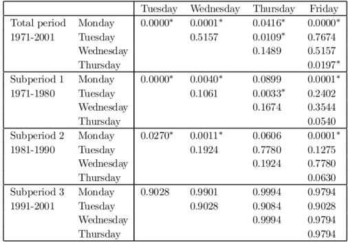
The FTSE 30 seems to exhibit the classical Monday e¤ect in the total period, since Monday returns are statistically distinguishable from all other days of the week. Furthermore, the equality of Thursday returns with Tuesday and Friday returns can be rejected. For the 1970’s and 1980’s we cannot reject the equality of Monday and Thursday returns as well as the equality of Thursday and Friday returns. While Tuesday and Thursday returns di¤er signi…cantly in the …rst subperiod their equality cannot be rejected at very high signi…cance levels for subperiod 2. The global null hypothesis has already ruled out any day-of-the-week e¤ect for the 1990’s.

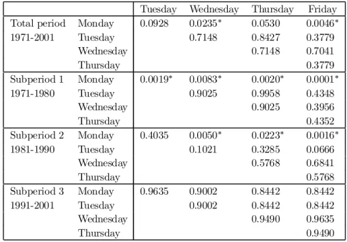
The analysis of the DAX 30 for the total period shows that Monday re- turns di¤er signi…cantly from Wednesday and Friday returns. In the 1970’s Monday returns are statistically distinguishable from all other days of the week. In the 1980’s the equality of Monday and Tuesday returns cannot be rejected any longer. Subperiod 3 has already been found not to exhibit any day-of-the-week e¤ect.

Since the main focus of our work is the test design we choose to restrict our presentation here to the results obtained by standard OLS estimation.

In additional computations we account for heteroscedasticity by using the White correction when estimating the regression equation and allow for non- normality by using a more general chi-square test instead of the standard

F-Test.⁴ The non-standard results further weaken the evidence of a day-of- the-week e¤ect in the US stock market. H₀cannot be rejected anymore for the total period, which means that there is no evidence for a day-of-the-week e¤ect relating to the period 1971-2001. Results concerning pairwise compar- isons are quite similar to the ones reported. In addition to the di¤erences found already we see signi…cant di¤erences between Thursday and Friday returns for the 1970’s and 1980’s in the FTSE 30. Furthermore, the equality of Tuesday and Friday returns in the 1980’s can be rejected for the DAX 30.

An interesting question that remains is whether the closure test principle and the conventional test methodology yield qualitatively di¤erent results.

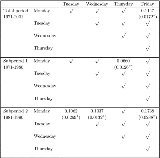
Tables 7 to 9 present p-values corresponding both to the closure test principle (upper value) and to the conventional approach (lower value in brackets), whenever a rejection of the primary hypothesis (based on the conventional approach) would have been the wrong conclusion.

In case of the S&P 500, the conventional approach would have yielded a di¤erent conclusion once for the total period and the …rst subperiod and three times for subperiod two. If we look at the primary hypothesis that Monday returns equal Friday returns in the total period, the adjusted p- value of 0.1147 does not reject the null hypothesis, whereas the conventional p-value of 0.0172 does reject.

While conventional testing would have found a Monday e¤ect over the …rst two subperiods in the UK market, Monday returns are indistinguishable from Thursday returns when considering adjusted p-values. The same holds true for the comparison of Thursday and Friday returns.

Monday returns are no longer signi…cantly di¤erent from Tuesday and Thurs-

4Results are available on request.

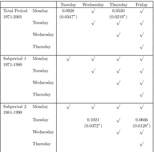
day returns when adopting the closure test principle for the DAX 30 data.

Including the subperiods there are four cases where conventional testing would have lead to a di¤erent conclusion. For example, looking at the sec- ond subperiod we would have rejected the equality of Tuesday returns to Wednesday and Friday returns, although not all subhypotheses can be re- jected.

p-value

Primary hypothesis H₁₂: °₁ =°₂ 0.046^¤ (adjusted)

Subhypotheses H12: °₁ =°₂ 0.012^¤

H₁₂₃: °₁ =°₂ =°₃ 0.008^¤ H₁₂₄: °₁ =°₂ =°₄ 0.040^¤ H₁₂₅: °₁ =°₂ =°₅ 0.019^¤ H₁₂₃₄: °₁=°₂ =°₃ =°₄ 0.021^¤ H1235: °₁=°₂ =°₃ =°₅ 0.018^¤ H₁₂₄₅: °₁=°₂ =°₄ =°₅ 0.046^¤ H_12;34: °₁ =°₂^°₃ =°₄ 0.017^¤ H_12;35: °₁ =°₂^°₃ =°₅ 0.037^¤ H_12;45: °₁ =°₂^°₄ =°₅ 0.029^¤ H_123;45: °₁=°₂ =°₃^°₄ =°₅ 0.016^¤ H_124;35: °₁=°₂ =°₄^°₃ =°₅ 0.018^¤ H125;34: °₁=°₂ =°₅^°₃ =°₄ 0.021^¤ H_345;12: °₃=°₄ =°₅^°₁ =°₂ 0.043^¤ H₁₂₃₄₅=H₀: °₁ =°₂ =°₃=°₄=°₅ 0.034^¤ Table 3: Example of a Set of Subhypotheses.

The table lists p-values for the primary null hypothesisH₁₂and the set of all subhypotheses for the S&P 500, 1971-2001. The …rst value is the adjusted p-value, while the other values are traditional p-values.

* indicates signi…cance at the 5 % level.

Tuesday Wednesday Thursday Friday Total period Monday 0.0459^¤ 0.0427^¤ 0.4545 0.1147

1971-2001 Tuesday 0.8931 0.5986 0.8970

Wednesday 0.5986 0.8931

Thursday 0.6601

Subperiod 1 Monday 0.0122^¤ 0.0012^¤ 0.0660 0.0016^¤

1971-1980 Tuesday 0.6157 0.8967 0.6157

Wednesday 0.4705 0.9396

Thursday 0.4705

Subperiod 2 Monday 0.1062 0.1037 0.5493 0.1738

1981-1990 Tuesday 0.9502 0.7365 0.9885

Wednesday 0.7365 0.9502

Thursday 0.7365

Subperiod 3 Monday 0.8794 0.6869 0.6652 0.6193

1991-2001 Tuesday 0.8686 0.8686 0.8468

Wednesday 0.9500 0.8794

Thursday 0.8794

Table 4: Test Results for the S&P 500.

The table presents adjusted p-values for hypotheses

H_ij :°_i =°_j; 1·i < j·5 for the total period and the three subperiods.

* indicates signi…cance at the 5 % level.

Tuesday Wednesday Thursday Friday Total period Monday 0.0000^¤ 0.0001^¤ 0.0416^¤ 0.0000^¤

1971-2001 Tuesday 0.5157 0.0109^¤ 0.7674

Wednesday 0.1489 0.5157

Thursday 0.0197^¤

Subperiod 1 Monday 0.0000^¤ 0.0040^¤ 0.0899 0.0001^¤

1971-1980 Tuesday 0.1061 0.0033^¤ 0.2402

Wednesday 0.1674 0.3544

Thursday 0.0540

Subperiod 2 Monday 0.0270^¤ 0.0011^¤ 0.0606 0.0001^¤

1981-1990 Tuesday 0.1924 0.7780 0.1275

Wednesday 0.1924 0.7780

Thursday 0.0630

Subperiod 3 Monday 0.9028 0.9901 0.9994 0.9794

1991-2001 Tuesday 0.9028 0.9084 0.9028

Wednesday 0.9994 0.9794

Thursday 0.9794

Table 5: Test Results for the FTSE 30.

The table presents adjusted p-values for hypotheses

H_ij :°_i =°_j; 1·i < j·5 for the total period and the three subperiods.

* indicates signi…cance at the 5 % level.

Tuesday Wednesday Thursday Friday Total period Monday 0.0928 0.0235^¤ 0.0530 0.0046^¤

1971-2001 Tuesday 0.7148 0.8427 0.3779

Wednesday 0.7148 0.7041

Thursday 0.3779

Subperiod 1 Monday 0.0019^¤ 0.0083^¤ 0.0020^¤ 0.0001^¤

1971-1980 Tuesday 0.9025 0.9958 0.4348

Wednesday 0.9025 0.3956

Thursday 0.4352

Subperiod 2 Monday 0.4035 0.0050^¤ 0.0223^¤ 0.0016^¤

1981-1990 Tuesday 0.1021 0.3285 0.0666

Wednesday 0.5768 0.6841

Thursday 0.5768

Subperiod 3 Monday 0.9635 0.9002 0.8442 0.8442

1991-2001 Tuesday 0.9002 0.8442 0.8442

Wednesday 0.9490 0.9635

Thursday 0.9490

Table 6: Test Results for the DAX 30.

The table presents adjusted p-values for hypotheses

H_ij :°_i =°_j; 1·i < j·5 for the total period and the three subperiods.

* indicates signi…cance at the 5 % level.

Tuesday Wednesday Thursday Friday

Total period Monday p p p _0.1147

1971-2001 (0.0172^¤)

Tuesday p p p

Wednesday p p

Thursday p

Subperiod 1 Monday p p

0.0660 p

1971-1980 (0.0126^¤)

Tuesday p p p

Wednesday p p

Thursday p

Subperiod 2 Monday 0.1062 0.1037 p

0.1738 1981-1990 (0.0269^¤) (0.0132^¤) (0.0288^¤)

Tuesday p p p

Wednesday p p

Thursday p

Table 7: Closure Test Principle and Conventional Testing, S&P 500.

The table shows a comparison of test results on the basis of the closure test principle (adjusted p-value) and conventional testing (traditional p-value in brackets).

* indicates signi…cance at the 5 % level. p indicates same result for both testing approaches.

Tuesday Wednesday Thursday Friday

Total Period Monday p p p p

1971-2001

Tuesday p p p

Wednesday p p

Thursday p

Subperiod 1 Monday p p _0.0899 p

1971-1980 (0.0466^¤)

Tuesday 0.1061 p p

(0.0346^¤)

Wednesday p p

Thursday 0.0540

(0.0167^¤)

Subperiod 2 Monday p p _0.0606 p

1981-1990 (0.0233^¤)

Tuesday p p _0.1275

(0.0476^¤)

Wednesday p p

Thursday 0.0630

(0.0203^¤) Table 8: Closure Test Principle and Conventional Testing, FTSE 30.

The table shows a comparison of test results on the basis of the closure test principle (adjusted p-value) and conventional testing (traditional p-value in brackets).

* indicates signi…cance at the 5 % level. p indicates same result for both testing approaches.

Tuesday Wednesday Thursday Friday

Total Period Monday 0.0928 p _0.0530 p

1971-2001 (0.0347^¤) (0.0219^¤)

Tuesday p p p

Wednesday p p

Thursday p

Subperiod 1 Monday p p p p

1971-1980

Tuesday p p p

Wednesday p p

Thursday p

Subperiod 2 Monday p p p p

1981-1990

Tuesday 0.1021 p _0.0666

(0.0372^¤) (0.0128^¤)

Wednesday p p

Thursday p

Table 9: Closure Test Principle and Conventional Testing, DAX 30.

The table shows a comparison of test results on the basis of the closure test principle (adjusted p-value) and conventional testing (traditional p-value in brackets).

* indicates signi…cance at the 5 % level. p indicates same result for both testing approaches.

6 Conclusion

A drawback of many empirical studies of market anomalies is that the mul- tiplicity e¤ect is not accounted for appropriately or even ignored completely.

This may result in an in‡ated occurrence of type I errors producing spurious signi…cance with regard to the test results. To overcome this problem, we propose a special type of multiple test procedure based on the closure test principle introduced by Marcus, Peritz and Gabriel (1976). This procedure, which has strongly in‡uenced the …eld of multiple hypotheses testing in re- cent decades, seems to be quite unknown in the …nancial literature. The underlying principle guarantees the construction of test procedures with the property that the probability of rejecting at least one of the true null hy- potheses is always smaller than or equal to a given level ®, independent of how many and which null hypotheses are actually true. For further results on closed test procedures see, for example, Hochberg and Tamhane (1987), Hsu (1996) or Pigeot (2000).

In our paper we apply the closure test principle to test for day-of -the-week e¤ects in the U.S., the British and the German stock market during the period 1971 to 2001, including three subperiods. Our results con…rm the existence of a day-of-the-week e¤ect for the total and the …rst subperiod in all markets, and for the second subperiod in the British and German market only, though not as pronounced as documented in other studies. We …nd no evidence for a day-of-the-week e¤ect during the 1990’s. In contrast to other studies we examine all pairwise comparisons of expected week-day returns and do not restrict ourselves to anomalies a¢liated with Monday returns.

We also compare test decisions resulting from the closed test procedure and conventional testing. In some cases conventional testing rejects pairwise

equalities, while according to the closure test principle the pairwise equality cannot be rejected. One has to keep in mind that conventional testing does not guarantee that type I error probabilities are less or equal than ®.

A …nal point worth mentioning is the fact that the closure test principle is not only a generally applicable method for constructing multiple level ® tests.

It can also be used to characterize these procedures. Under the assumption that no primary hypothesis is a proper subset of any other, one can show that for each multiple level® test there exists a closed test procedure, such that the test decisions of both procedures coincide with respect to the primary null hypothesesH₀₁; :::; H_0n. This implies that under the assumption stated above, a test procedure keeps the multiple level ®if and only if there exists an ’equivalent’ closed test procedure. In particular this result holds for the case of testing the multiple comparisons Hij: °_i =°_j;1·i < j·5, which we used to test for day-of-the-week e¤ects.

References

[1] Chang, E. C.; J. M. Pinegar; and R. Ravichandran. ”International Ev- idence on the Robustness of the Day-of-the-Week E¤ect”, Journal of Financial and Quantitative Analysis, 28 (1993), 497-513.

[2] Chow, K.V, and K. Denning. ”A Simple Multiple Variance Ratio Test”, Journal of Econometrics, 58 (1993), 385-401.

[3] Cross, F. ”The Behaviour of Stock Prices on Friday and Monday”, Financial Analysts Journal, 29 (1973), 67-69.

[4] Connolly, R.A. ”A Posterior Odds Analysis of the Weekend E¤ect”, Journal of Econometrics, 49 (1991), 51-104.

[5] Dubois, M., and P. Louvet. ”The Day-of-the-Week E¤ect: The Inter- national Evidence”,Journal of Banking and Finance, 20 (1996), 1463- 1484.

[6] French, K. R. ”Stock Returns and the Weekend E¤ect”, Journal of Financial Economics, 8 (1980), 55-69.

[7] Greenstone, M., and P. Oyer. ”Are There Sectoral Anomalies Too?

The Pitfalls of Unreported Multiple Hypothesis Testing and a Simple Solution”, Review of Quantitative Finance and Accounting, 15 (2000), 37-55.

[8] Hochberg, Y., and A.C. Tamhane. Multiple Comparison Procedures, New York: John Wiley (1987).

[9] Hsu, J.C. Multiple Comparisons, London: Chapman & Hall (1996).

[10] Huber, P. ”Stock Market Returns in Thin Markets: Evidence from the Vienna Stock Exchange”,Applied Financial Economics, 7 (1997), 493- 498.

[11] Ja¤e, J. F., and R. Wester…eld. ”The Week-End E¤ect in Common Stock Returns: The International Evidence”, Journal of Finance, 40 (1985), 433-454.

[12] Keim, D. B., and R.F. Stambaugh. ”A Further Investigation of the Weekend E¤ect in Stock Returns”,Journal of Finance, 39 (1984), 819- 835.

[13] Madlener, R., and R. Alt. ”Residential Energy Demand Analysis: An Empirical Application of the Closure Test Principle”, Empirical Eco- nomics, 21 (1996), 203-220.

[14] Marcus, R.; E. Peritz; and K.R. Gabriel. ”On Closed Testing Proce- dures with Special Reference to Ordered Analysis of Variance”, Bio- metrika, 63 (1976), 655-660.

[15] Neusser, K. ”Testing the Long-Run Implications of the Neoclassical Growth Model”,Journal of Monetary Economics, 27 (1991), 3-37.

[16] Pigeot, I. ”Basic Concepts of Multiple Tests - A Survey”, Statistical Papers, 41 (2000), 3-36.

[17] Savin, N.E. ”Multiple Hypothesis Testing.” In: Handbook of Economet- rics (1984), Vol. II, Z. Griliches and M.D. Intriligator, eds. Amsterdam:

North-Holland.

[18] Sullivan, R.; A. Timmermann; and H. White. ”Dangers of Data Mining:

The Case of Calendar E¤ects in Stock Returns”,Journal of Economet- rics, 105 (2001), 249-286.

Authors: Raimund Alt, Ines Fortin, Simon Weinberger

Title: The Day-of-the-Week Effect Revisited: An Alternative Testing Approach

Reihe Ökonomie / Economics Series 127

Editor: Robert M. Kunst (Econometrics)

Associate Editors: Walter Fisher (Macroeconomics), Klaus Ritzberger (Microeconomics)

ISSN: 1605-7996

© 2002 by the Department of Economics and Finance, Institute for Advanced Studies (IHS),

Stumpergasse 56, A-1060 Vienna • ( +43 1 59991-0 • Fax +43 1 59991-555 • http://www.ihs.ac.at