Bismarck to no effect: Fertility decline and the introduction of social insurance in Prussia

Working Papers of the Priority Programme 1859

Experience and Expectation.

Historical Foundations of Economic Behaviour

Edited by Alexander Nützenadel und Jochen Streb

No 13 (2019, December)

Working Papers of the Priority Programme 1859

„Experience and Expectation. Historical Foundations of Economic Behaviour”

No 13 (2019, December)

Guinnane, Timothy W. / Streb, Jochen

Bismarck to no effect: Fertility decline and the

introduction of social insurance in Prussia

Arbeitspapiere des Schwerpunktprogramms 1859 der Deutschen Forschungsgemeinschaft

„Erfahrung und Erwartung. Historische Grundlagen ökonomischen Handelns“ / Working Papers of the German Research Foundation’s Priority Programme 1859

“Experience and Expectation. Historical Foundations of Economic Behaviour”

Published in co-operation with the documentation and publication service of the Humboldt University, Berlin (https://edoc.hu-berlin.de).

ISSN: 2510-053X

Redaktion: Alexander Nützenadel, Jochen Streb, Ingo Köhler V.i.S.d.P.: Alexander Nützenadel, Jochen Streb

SPP 1859 "Erfahrung und Erwartung. Historische Grundlagen ökonomischen Handelns"

Sitz der Geschäftsführung:

Humboldt-Universität

Friedrichstr. 191-193, 10117 Berlin

Tel: 0049-30-2093-70615, Fax: 0049-30-2093-70644 Web: https://www.experience-expectation.de Koordinatoren: Alexander Nützenadel, Jochen Streb Assistent der Koordinatoren: Ingo Köhler

Recommended citation:

Guinnane, Timothy W. / Streb, Jochen (2019): Bismarck to no effect: Fertility decline and the introduction of social insurance in Prussia. Working Papers of the Priority Programme 1859 “Experience and Expectation.

Historical Foundations of Economic Behaviour” No 13 (December), Berlin

© 2019 DFG-Schwerpunktprogramm 1859 „Erfahrung und Erwartung. Historische Grundlagen ökonomischen Handelns“

The opinions and conclusions set forth in the Working Papers of the Priority Programme 1859 Experience and Expectation. Historical Foundations of Economic Behaviour are those of the authors. Reprints and any other use for publication that goes beyond the usual quotations and references in academic research and teaching require the explicit approval of the editors and must state the authors and original source.

1

Bismarck to no effect: Fertility decline and the introduction of social insurance in Prussia

Timothy W. Guinnane Yale University

Jochen Streb University of Mannheim

December 2019

Abstract

Economists have long argued that introducing social insurance will reduce fertility. The hypothesis relies on standard models: if children are desirable in part because they provide security in case of disability or old age, then state programs that provide insurance against these events should induce couples to substitute away from children in the allocation of wealth. We test this claim using the introduction of social insurance in Germany in the 1880s and 1890s. Bismarck’s social-insurance system provided health insurance, workplace-accident insurance, and old age pensions to a majority of the working population. The German case appeals because the social insurance program started on a large scale and was compulsory for covered classes of workers, and because fertility in Germany in this period was still relatively high. Focusing on the state of Prussia, we estimate differences-in-differences models that ask whether marriage and marital fertility reacted to the introduction or extension of the main social insurance programs. For Prussia as a whole we find little impact.

JEL classification: J13, H55, N33

Keywords: fertility transition, marriage pattern, old-age pension, health insurance, accident insurance Adresses: timothy.guinnane@yale.edu; streb@uni-mannheim.de

Note: This discussion paper does not include the appendices, which are available upon request. For comments and suggestions we thank Martha J. Bailey, Alexander Donges, Tobias Jopp, Joshua Lewis, Katerina Piro, Paul W. Rhode, Ebonya Washington, and seminar participants at the University of Adelaide, the Australian National University, the University of Melbourne, the University of Connecticut, the Vienna University of Economics and Business, the XVIII World Economic History Conference at Boston in August 2018, and the IEHA meeting in Paris in November 2019. The German Science Foundation (DFG) funded this project as part of the Priority Program 1859 “Experience and Expectations: Historical Foundations of Economic Behavior.” Guinnane thanks the Economic Growth Center (Yale University) for additional funding. We are grateful to the student assistants who helped to collect and organize the data.

2 Figures

1. Births, deaths and marriages in Prussia, 1880-1910……….5

2. Changes in marriage and legitimate fertility in Prussia, 1875-1910……….8

3. Coverage under the health insurance system (1884)………...15

4. The three stages of accident-insurance………16

5. Coverage under the old-age Pension (1891)………17

6. The effect of social insurance on marriage, all of Prussia………...26

7. The effect of social insurance on fertility, all of Prussia……….27

8. The effect of social insurance on marriage, in western and eastern Prussia………29

9. The effect of social insurance on fertility, in western and eastern Prussia………..30

Tables 1. Contributions and benefits under the social-insurance system……….9

2. Occupational groups defined by treatment status………11

3. Treatment groups in three example districts´………..20

3

Economists have often argued that the introduction of social insurance could reduce the demand for children. If children represent a form of savings and insurance against the vicissitudes of life, providing alternative insurance should induce adults to substitute away from children. Today some scholars advocate social insurance to reduce the demand for children in high-fertility countries. The decline of fertility in wealthy countries, on the other hand, is often understood as an unwanted consequence of generous social insurance systems. The social-insurance/fertility nexus has a particularly undesirable consequence in countries that finance social-insurance expenditure out of current contributions (pay-as-you-go) because population aging, which is a consequence of low fertility, raises individual fiscal burdens for the shrinking group of working adults.¹ We focus on the introduction of Bismarck’s social-insurance system in the 1880s and 1890s to ask whether the introduction of the world’s first large social-insurance schemes reduced fertility. We find little effect.

The second half of the nineteenth century in Europe witnessed two of the great transformations that created our world. One was demographic. Europeans began to marry at earlier ages and in larger proportions than in the past. Women had fewer children, and more of those children survived childhood. The introduction of social insurance marked a second transformation: to supplant locally organized and financed, highly discretionary programs, European governments introduced national schemes that provided well- defined benefits triggered by events such as illness, accident, or old age. This paper studies the effect of the second transformation on the first. German Chancellor Otto von Bismarck’s three-pillar program of health insurance, workplace accident insurance, and old age pensions was among the earliest and most extensive of European social-insurance programs. The system covered virtually all workers in specific sectors, and, over time, included most of the workforce. German social insurance appeared with a bang: compulsory health- and accident-insurance programs created in 1883 and 1884 covered some 29 and 50 percent of all workers, respectively, and the pension insurance (1891) initially applied to 58 percent of workers. We focus

1 Schultz (1997) surveys the evidence on the demand for children in low-income countries. Becker and Barro (1988) focus on the fertility-reducing incentives in a pension scheme. Sinn (2004) argues that the pay-as-you-go pension system serves both as insurance against not having children and as an enforcement device for ungrateful children who are unwilling to support their aged parents.

4

on the state of Prussia, which accounted for about two-thirds of the entire German population in 1880. The insurance rules were common to all the German states, and Prussia has high-quality demographic and other data that justify restriction to this state.

The introduction of social insurance in Germany offers a chance to study the demographic impact of social insurance free from some important complicating influences. Bismarck pushed social insurance to achieve larger political goals, including alienating the German working class from social democracy. No major economic crisis took place in the period we study, and, Germany experienced peace until 1914.² Studies of social insurance’s impact in other countries, on the other hand, present complications because of program design or the historical context of introduction. The U.K.’s old age pensions (1908), for example, was at first means-tested and thus affected only parts of the population. The U.S. Social Security system (enacted in 1935) has also received considerable attention. The U.S. program was simpler than its U.K.

counterpart, but came into being during the Great Depression.³

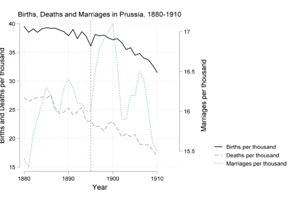
The demographic context also provides a more realistic test in the German case. By 1908 (for the U.K.) and especially by 1935 (for the U.S.), fertility had already declined considerably.⁴ Because Bismarck’s system appeared relatively early, fertility was much higher at the time of program introduction than in the U.K. or the U.S. Figure 1 reports the crude birth rate and crude marriage rate for Prussia for 1880 to 1910. From 1880 to 1895, the crude birth rate declined by about ten percent; the pace of decline picked up thereafter.⁵ Figure 1 also reveals that marriage rates increased in the late nineteenth century. The latter development is usually explained by the relaxation of marriage restrictions that we describe below.

2For the political dimensions of the social-insurance program see Wehler (1995, pp. 907-915) and Frerich and Frey (1996, p. 91). An earlier historiography viewed the 1880s as a “Great Depression,” but that view reflected a confusion of falling prices with falling real output. Hoffmann (1965)’s and Burhop and Wolff (2005)’s GDP estimates imply steady growth throughout the 1880s. Burhop and Wolff (2005, Figure 16) see the late 1870s and 1880s as a business- cycle upswing.

3 For both the U.K. and the U.S., the advent of a world war soon after program introduction also complicates efforts to understand these programs’ long-term impacts.

4 The Total Fertility Rate (TFR) measures the number of children a woman would bear in her lifetime if she survived to the end of child-bearing years and experienced the current age-specific fertility at each age. According to Coale and Zelnik (1963, Table 2), the TFR for the white U.S. population first fell below 3.0 in 1922, was 2.6 in 1928 (before the onset of the Depression), and by 1935 was 2.14. David and Sanderson (1987) argue that for decades U.S. birth- controllers had shown strong evidence of a two-child norm. Fertility of African-Americans was higher, in part because they were at this point more rural, but the trends are similar to whites (Coale and Rives (1973)).

5 Marschalk (1984, p. 157) reports TFR for Germany as a whole in 1881/90 as 4.93 and in 1891/1900 as 4.78.

5

Figure 1: Births, Deaths and Marriages in Prussia, 1880-1910

Researchers have only recently considered the German social insurance system’s implications.⁶ Jopp (2011, 2012, 2013) studies the earlier miner’s social-insurance system (the Knappschaften) which was the model for Bismarck’s program. Fenge and Scheubel (2017) (which builds on Scheubel (2013)) marks the first empirical test of the social-insurance/fertility nexus for Germany. They claim that the introduction of old age pensions in 1891 accounts for 15 percent of the observed fertility decline in the German Empire in the late nineteenth century. We, in contrast, find essentially no effect. These contradictory results reflect different methods as well as our focus on Prussia alone. Our approach differs from Fenge and Scheubel (2017) in four essential ways. First, we study demographic decisions at the level of 450 Prussian Kreise, a small unit comparable to a U.S. county, with an average population of about 62 thousand in 1880. Fenge and Scheubel (2017) on the other hand, (building on Scheubel (2013)) employ as their units of analysis the

6 Jäger (2017) studies the impact of public pensions on fertility in several European countries. He uses aggregate, national-level data on fertility and ascribes all effects to the year a program was introduced. Germany is not in his dataset.

6

twenty-three districts (German states and provinces) corresponding to the social-insurance authority’s administrative divisions in most of Germany. These districts had an average population of 2.2 million people.⁷ Second, we use differences-in-differences to estimate the demographic impact of Bismarck’s complete social-insurance system, a scheme that included generous health and workplace-accident insurance in addition to the old-age pension. Fenge and Scheubel (2017) focus on the last part of the program, the old-age pension introduced in 1891. Third, the social-insurance scheme affected incentives to marry independently of incentives to have children, so we consider marriage and fertility separately. Fenge and Scheubel (2017) do not consider marriage patterns. Finally, we estimate econometric models for the period from 1880 to 1995 to understand how the system’s roll-out affected demographic decisions made by covered workers. Fenge and Scheubel (2017) use the two years 1895 and 1907. These later years saw the acceleration of Germany’s fertility decline. By limiting themselves to these two years, they make implicit assumptions about when individuals reacted to the new social-insurance system.

Elsewhere we have studied other implications of Bismarck’s program. Guinnane and Streb (2015) demonstrate that accidence insurance decreased the number of workplace accidents. Lehmann-Hasemeyer and Streb (2018) show that social security crowded out private savings, just as has been argued for the U.S.

social security system (Feldstein 1974). Bauernschuster et al (2019) consider the health insurance system’s effect on health outcomes per se. Khoudour-Castéras (2008) shows that workers valued social insurance in the sense that for a given American-German wage differential, German emigration rates became smaller after 1883. A much larger literature discusses related issues in other countries. The best-developed case is the United States, for which Fishback, Kantor, and co-authors have studied several issues related to the design and execution of the workmen’s compensation system (the U.S. analogue of Germany’s accident insurance system) as well as a broader range of questions dealing with relief programs under Roosevelt’s

“New Deal.”⁸

7Fenge and Scheubel’s units span Germany, while we focus on Prussia alone. Prussia had 35 Regierungsbezirke, administrative units larger than Kreise but much smaller than those used by Fenge and Scheubel. In 1884, about one- third of the variation among Kreise in the marriage and fertility measures were within the Regierungsbezirk.

8 Fishback et al (2007) study the effect of relief policies during the Great Depression, and thus is thematically closest to this paper. They contend with a much richer and more complicated set of policies than characterized German social

7 Germany’s fertility transition

The demographic changes we study took place within a larger context. Fertility decline was pan- European; an explanation of fertility decline cannot rest solely on some fact peculiar to Germany. Princeton University’s European Fertility Project (EFP) implies that the German fertility transition began in the 1870s or 1880s. The EFP relied on highly aggregated data and a particular set of indices. Other studies that rely on individual-level fertility histories have found evidence of fertility control earlier in the nineteenth century.⁹ We need not take a position on the details underlying these discrepancies. For us, the key point is that by 1880, the fertility transition in Germany was clearly underway.

Testing the effect of social insurance on fertility requires attention to an important feature of the demographic regime. At least as far back as Malthus, scholars have noted that Europeans controlled births in aggregate by limiting access to marriage and stigmatizing illegitimate births to single mothers. Rather than controlling marital fertility, the number of children born to married couples, Europeans controlled nuptiality.¹⁰ In most countries, as married couples reduced their fertility, young people began to marry earlier, and more of them married. Germany was no exception. In the period 1871-1910, the average age at marriage for both men and women fell by one year, and the proportion of both men and women who never married fell by about 15 percent. These changes in marriage patterns offset the decline in marital fertility significantly. A simple counter-factual calculation implies that the overall fertility decline in the period 1867-1910, about 20 percent, would have been 28 percent had marriage patterns not changed.¹¹

insurance in the early days. For the workman’s-compensation project see Fishback and Kantor (2007). See also Fishback et al (2010).

9 Knodel (1974) is the Princeton Project’s contribution on Germany. The EFP dated each country’s fertility transition as the first year for which marital fertility was at least ten percent below its observed maximum. See Guinnane et al (1994) for the limitations of this approach. Knodel (1988, Table 11.1) reports the Coale-Trussell “m” index of stopping for a selection of German villages. Couples in some of these communities controlled their fertility as early as 1800- 24; nearly all of the communities show evidence of control by the marriage cohorts 1825 to 1849.

10 The use of marriage to control fertility reflects either reluctance to use available contraceptive methods, the expense and unreliability of the methods available, or fixed costs to establishing new households. For more on the fertility transition and the pre-transition regime, see Guinnane (2011). For an elegant statement of Malthusian thinking, see Wrigley and Schofield (1981).

11 According to Knodel (1974, Table 2.14), male age at first marriage declined from 28.8 to 27.9, and female age at marriage from 26.3 to 25.3. Proportions never-married at age 50 fell from 9.3 to 7.9 percent for males and 11.9 to 10.4 percent for females. The counter-factual calculation in the text uses the EFP indices as reported in Knodel (1974, Table

8

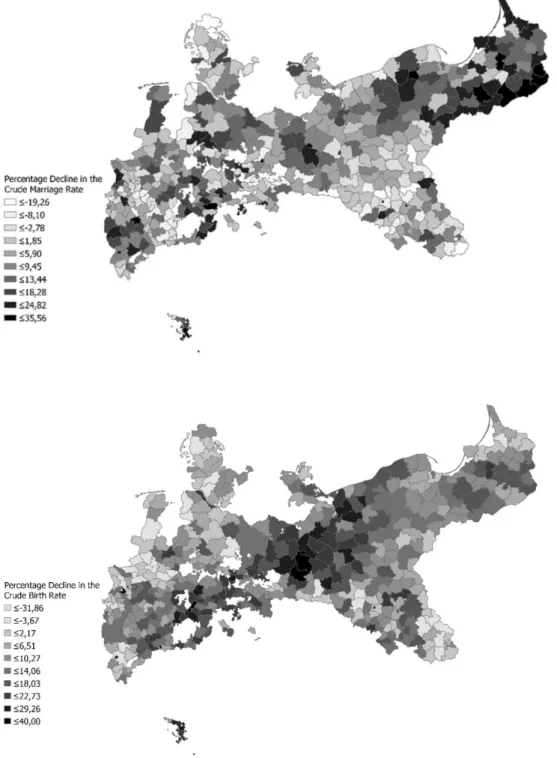
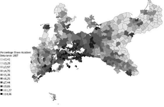
Figure 2: Changes in marriage and legitimate fertility in Prussia, 1875-1910

Note: The white areas correspond to territories that were not part of Prussia.

2.1); we re-compute “If” for 1910 using the 1910 value of Ig and the 1867 value of Im. To appreciate the importance of an apparently small reduction in the mean age at marriage, consider that the age-specific annual marital fertility rate would be in the range .4-.5 births for women in their twenties (see, for example, Knodel (1974, Table 10.2)).

9

Figure 2 reports the decline in legitimate Crude Birth Rates (CBR) and Crude Marriage Rates (CMR) from 1875-1910 in Prussian Kreise.¹² (The darker areas correspond to larger fertility and nuptiality reductions.) The cross-sectional patterns demonstrate the complexity of demographic change in this period.

Throughout this paper, we treat marriage and marital fertility separately, reflecting two distinct potential channels from the social-insurance programs.

Three pillars of social insurance

All three pillars extended compulsory coverage to workers defined by occupational groups. Table 1 summarizes each scheme’s contributions and benefits. Each program differed in the benefits it offered and the financing of its costs. Table 2 lists the occupation groups included in each round of the system’s extension, including those that took place after our period. The groups A-G aggregate these occupations into treatment groups discussed below.

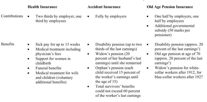
Table 1: Contributions and benefits under the social insurance system

Health Insurance Accident Insurance Old Age Pension Insurance Contributions  Two thirds by employer, one

third by employees  Fully by employers  One half by employers, one half by employees

 Additional governmental subsidy (50 marks per pensioner)

Benefits  Sick pay for up to 13 weeks

 Medical treatment including physician’s fees

 Support for women in childbirth

 Funeral benefits

 Medical treatment for wife and children (voluntary additional benefits)

 Disability pension (up to two thirds of the last earnings)

 Widow’s pension (20 percent of her husband’s last earnings) until she remarried

 Orphan’s pension (each child received 15 percent of the worker’s earnings until the age of 15)

 Total survivors’ benefits could not exceed 60 percent of the worker’s last earnings

 Disability pension (approx. 20 percent of the last earnings¹)

 Old age pension at age of 70 (approx. 20 percent of the last earnings¹)

 Widow’s pension for white- collar workers after 1912, for blue-collar workers after 1927

* Frerich, Johannes and Martin Frey (1996): Handbuch der Geschichte der Sozialpolitik in Deutschland, Vol. 1: Von der vorindustriellen Zeit bis zum Ende des Dritten Reiches, Oldenbourg Verlag, Munich/Vienna, p. 106.

12 We stress crude rates for data reasons discussed below. Figure 2 reports that CBR rose in some districts. This is

entirely possible, even if age-specific marital fertility rates declined, because the measure does not control for age- structure or marital status.

10

The health insurance system (which came into effect in 1884) relied on thousands of funds that organized medical insurance in their region. Benefits included partial replacement pay for those unable to work because of illness as well as doctor’s fees, hospitalization, and drugs and other therapies. Workers split the cost of their medical coverage with their employers. The law permitted health insurance funds to extend benefits to the spouses and children of covered workers. Unfortunately, we do not have data on how common this practice was; as late as 1914, only slightly more than half of sampled funds did so, suggesting the practice was a first rare.¹³

The accident insurance system created not-for-profit mutual insurance funds (Berufsgenossenschaften) that combined firms in similar industries into one organization. The funds provided partial replacement pay for covered persons unable to work because of an on-the-job injury.

Accident insurance also paid for medical care, hospitalization, rehabilitation, and other medical therapies.

Disabled workers received partial or full pensions, depending on their injury, and the system paid survivor benefits to widows and orphans. Benefits under this program could be substantial. A contemporary publication gives the example of a mason whose workplace accident left him fully disabled. Assuming an annual working income of 1,391.7 Marks, the insurance program would pay him 928.2 Marks annually for life, or 835.2 Marks annually to his widow if he died. Covered workers did not contribute financially to the accident-insurance system.¹⁴

The old age pension provided monthly payments to workers who had reached age 70 or who demonstrated a physical inability to earn a subsistence wage earlier in life. Bismarck’s social-insurance system distinguished two types of invalidity. The first type concerned invalidity caused by a workplace accident, and fell to the accident insurance system. The second type comprised all other causes of invalidity and was the responsibility of the old age pension insurance. Covered workers contributed to old-age pension;

13 Fifty-six percent of a sample of 325 local health insurance funds fully covered medical for spouses and children (Jahrbuch der Krankenversicherung, 1915, p. 218). See also Hausen (2013, p. 234).

14 The example is reported in Lass (1904, p. 15), which was printed for the 1904 St. Louis World’s Fair. Guinnane and Streb (2015) discuss the allocation of costs between the sickness and accident-insurance systems. An injured worker was temporarily the sickness fund’s responsibility. The legislation creating the accident insurance system undid an earlier liability system; covered workers could not sue their employers for damages.

11

contributions depended on working income, and benefits depended on their contributions. Mortality conditions at the time made reaching age 70 less likely than it is today. Ballod (1899, p.130) reports life expectancy at age 20 in the years 1890/91 of 37.3 years for men and 41.7 for women. Only about 30 percent of men aged 20 would survive to age 70, at which point they could expect another 7.3 years of life.¹⁵ Benefits under this third pillar were also meager. The average annual payment under both the disability and old age provisions was about 18 percent of the average worker’s wage in our period – far less than the accident-insurance system paid someone disabled in a workplace accident. Old-age pensions were at first more common than those the pension funds granted on the grounds of disability and on average paid slightly more. In 1895, about one in every 200 Germans received something from the 1891 program.¹⁶

Table 2: Occupational groups defined by treatment status

Group Who Insurance coverage Percent of all workers

(in 1882) A Industrial workers and white-collar workers Health insurance 1884

Accident insurance 1885 Pension insurance 1891

22.75

B Construction workers Health insurance 1884

Accident insurance 1887 Pension insurance 1891

4.43

C Farm workers (employees, not farmers) Accident insurance 1886 Pension insurance 1891

24.41

D Domestic servants Pension insurance 1891 8.1

E Public servants Government aid when sick or old

since 1825

Accident insurance 1886

1.0

F The self-employed, including farmers No social insurance in our period 36.23

G Miners Treated prior to Bismarck 3.06

Note: In group A, high-paid white-collar workers are included (although not treated) because we cannot distinguish them from low-paid white-collar workers in the statistics. See text for discussion of Group “D” especially. The final column is defined as in the regressions reported in the text.

15 The mortality figures are for mid-size cities (Mittelstädte). The survival number is for 1895-6. Fenge and Scheubel (2017, p.97) cite a different figure, which is for the cohort born in the year the old age pension was introduced.

16 For the pension in comparison to workers’ wages, see Kaschke and Sniegs (2001, Table A6, p.57). For numbers of pensions in force, Kaschke and Sniegs (2001, Table C1, p.96, and C12, p.135). The number of invalidity pensions spiked in the early twentieth century, to about 864 thousand in 1910 (compared to 96 thousand old-age pensions).

12

The three pillars covered all blue-collar workers in affected sectors. White-collar workers (Angestellte), on the other hand, came under the system only if their annual income did not exceed 2000 Marks. This income ceiling excluded few white-collar workers in our period. While we know of no estimates for the 1880s, Kocka (1981) reports that in 1903, 68.3 percent of male and 93.6 percent of female white- collar workers were covered by social insurance. Wage growth in the decade between the introduction of insurance and 1903 implies that relatively more white-collar workers were covered at outset.¹⁷

The demographic implications of social insurance

Each pillar affected marriage and fertility decisions differently. How would health insurance alone affect demographic decisions? Partial replacement pay and free medical care stabilized income for covered workers, and thus provided some inducement to marry and form a household. Note that this effect differs from standard Malthusian thinking, in which the demand for marriage is a positive function of the real wage.

However, the demand for marriage also depends on the second moment of real wages. This idea came up in connection with the earlier miner’s insurance (Jopp, 2011, 2012, 2013). A man who could provide for his family even when unable to work was a more attractive husband.¹⁸ Until the program extended coverage to children, however, health insurance did not change the marginal cost of an additional child to a married couple. Any effect on marital fertility must reflect the stabilization of the covered worker’s income.

The accident insurance system’s rules imply different effects on demographic decisions. The system stabilized worker incomes in the same way as health insurance. Severely-injured workers also received disability pay for life, and the system paid benefits to the widows and children of workers killed

17 White-collar workers in all were a small part of the workforce, 1.9 percent of the total in 1892 and 3.3 percent in 1895 (Kocka 1981, p.17, note 13). The estimate of insurance coverage appears on page 136, note 71.

18 Gegenüber dem Proletarier „verfügte der Bergmann über eine gesicherte Existenz und hinreichende Altersversorgung, […] er erfreute sich in weiten Kreisen der allgemeinen Hochschätzung und mochte daher, etwa bei der Brautwerbung, als junger Hauer erfolgreich auf die vielen Vorzüge seines Berufs hinweisen.“ (Tenfelde 1977, p.128) (Compared to the proletarian, "the miner had a secure existence and adequate retirement provision, [...] he enjoyed widespread general esteem and therefore, for example in courtship, drew attention to the many advantages of his job as a young miner") He quotes another author noting “das Ansehen des ‘ingeschriewenen’ Hauers als zuverlässigen Versorger der Familie“ (“the reputation of the ‘registered’ miner as a reliable provider for the family.”)(p.128, note 29).

13

on the job. This feature promoted marriage; a woman married to a covered worker knew that if her husband died on the job, she would receive payments for life.¹⁹ The incentives regarding marital fertility are more complex. Husbands and wives knew that his death on the job would not leave her with the burden of providing for their children, thus reducing the cost of children. On the other hand, because the accident insurance scheme included a pension, couples had incentives to reduce family sizes via the channel emphasized by economists for pensions. Given the countervailing effects, we cannot sign the net effect a priori.

The third pillar of Bismarck’s insurance system, the old age pension, theoretically promoted lower fertility for the reason articulated by economists: it provided for support in old age, making children less important for this purpose. There might be no countervailing effect in this case, but we need to bear in mind the program’s limitations.²⁰ The pension system applied to covered workers alone; widows and other survivors got nothing through this program. If the pension system affected marriage decisions, it was via the channel that made a man more valuable as a partner if he was entitled to a pension.

Estimation strategy

We study decisions at the level of the Kreis, a small unit comparable to a U.S. county. The average Kreis had a population of about 62 thousand in 1880. Our (entirely balanced) panel has one observation per Kreis for each year in the period 1880-1895. The 1882 census of occupations includes the number of workers in each sector in each Kreis. The census’s sector definitions (mostly) correspond to the groups included in the compulsory insurance system, so we use the 1882 figures to estimate the number of covered workers in each district. The program’s compulsory feature defines the intention to treat, which is the correct concept

19 Most insured workers were male, although covered women became relatively more numerous over time. Women accounted for 18 percent of insured under the health-insurance scheme in 1885, a figure that reached 37 percent in 1914. Women were 34 percent of pension insurees in 1904 (See Borscheid and Drees (1988); data available from the GESIS Datenarchiv, Cologne, histat, Studiennummer 8347 and 8602) See also Hausen (1995, p. 231).

20 Fenge and Scheubel (2017) note a different countervailing effect. Compulsory insurance forces households to purchase a substitute for children, thus reducing the demand for children. But the tax on household earnings reduces the value of time spent in market work, and thus decreases the opportunity cost of having and caring for children.

14

for our purposes: the question is whether the social insurance system altered expectations about the future in ways that changed demographic decisions.²¹

Bismarck’s system rolled out in stages. No Kreis was ever entirely untreated or entirely treated, so we identify program effects from differences in treatment intensity, measured as the fraction of workers covered under each round of the system. The three different pillars affected occupations differently, making it impossible to test the effect of any one pillar alone. When accident insurance came in 1885, it covered some workers already enrolled in the health insurance scheme and many who were not. We cannot estimate a pure “accident insurance” effect, for example, without assuming that accident insurance coverage affects everyone the same, regardless of their health insurance status. Rather, we create seven groups of occupations (A-G) defined by the complete package of coverage under the social insurance system. Group “A,” for example, consists of workers who received health insurance in 1883, accident insurance in 1884, and the pension system in 1891. Group “C’s” farm workers never had health insurance in our period, but were enrolled in accident insurance in 1886 and the pension system in 1891. Refer back to Table 2, which summarizes the coverage of workers in various sectors, including periods beyond those studied in this paper.²²

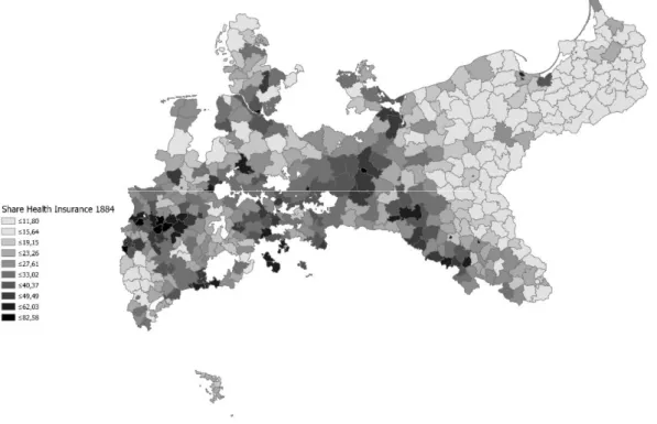
Figures 3-5 report the proportion of all workers covered at each stage. Miners enjoyed a sector- specific social insurance system prior to Bismarck’s program. Miners were most numerous in regions with rich deposits of coal and nonferrous metals, that is, the Rhineland, Westphalia, Saxony, and Silesia. The 1884 health-insurance map (Figure 3) shows that few workers in the eastern parts of Prussia received health insurance because uninsured farm workers dominated in this agricultural area characterized by large estates.

On the other hand, farm workers in eastern Prussia were the main beneficiaries of the second round of

21 Most program-evaluation studies estimate the effect of treatment, which combines both the offer to treat and actual participation in the program. Since the German system was compulsory for covered classes of workers, the difference between intention-to-treat effect and a treatment effect is less clear than in programs where eligible individuals may decline to participate. Heckman et al (1999, p.1903) note that the intention to treat is “is informative on how the availability of a program affects participant outcomes.”

22 The Gesetz, betreffend die Pensionierung und Versorgung der Militärpersonen, sowie die Bewilligung für die Hinterbliebenen of June 27, 1871 provided that, depending on their rank, officers and enlisted soldiers were eligible for invalidity and old age pensions up to 75 percent of their pay. Eligible individuals are not a large group (unlike the veterans of twentieth-century wars). Our analysis groups the military with others covered state employees.

15

accident insurance (Figure 4).²³ The accident-insurance system’s three-stage roll-out was not driven by contemporaries’ political preferences. The first round, 1884, replaced the Liability Act of 1871 that had focused on factory workers. The two later extensions were part of the original plan and the necessary legislation followed as intended (Ayaß, 2001, p. XVII).

Figure 3: Coverage under the health insurance system (1884)

Note: White areas correspond to territories that were not part of Prussia.

23 The occupational classes that appear in the 1882 census of occupations do not serve us well in one particular case.

The designation “Hausdienst und wechselnde Lohnarbeit” includes both domestic (household) servants and live-in farm workers (Gesinde). The former were definitely not included in the health and accident insurance systems in our period. The latter were covered under the 1886 accident insurance extension. Because we cannot distinguish the two groups in the 1882 enumeration, we assume, for the estimates reported in the text, that none of the individuals reported in this occupational group had insurance. Appendix C reports robustness checks in which we assume that large fractions of people reported in this category in rural areas were farm workers and thus were covered.

16 Figure 4: The three stages of accident insurance

17

Note: White areas correspond to territories that were not part of Prussia

Figure 5: Coverage under the old age pension (1891)

Note: white areas correspond to territories not part of Prussia.

18

Insurance coverage in each Kreis reflects uniform national rules and their interaction with local occupational structure. Differences in coverage between two Kreise do not mirror efforts to reward or punish specific classes of people. Our approach demands that the industrial structure in a given Kreis affected changes in demographic decisions only via inclusion in the insurance program. Since we stress fixed-effect models, a violation would require some type of change over time, within industries, that influenced the incentive to marry and to have children. Even then, to affect our results, such changes would have to be correlated with treatment intensity. Over a longer period than we cover, a sector’s waxing or waning fortunes might indeed affect marriage and fertility directly, but not in the short run we stress.

The fact that our treatment variables rely on cross-sectional differences in employment structure raises concerns about the role of migration. Some industries grew faster than others, and Kreise with fast growing industries such as Berlin or the Ruhr region attracted many migrants from less-developed parts of Prussia. Because of this structural change, the Kreis-level occupational distribution changed slightly from 1882 to 1895.

Our estimation strategy does not entirely obviate one particular form of workers’ self-selection.

Suppose there were two types of workers, those who were willing to pay for insurance and those who were not. When the accident-insurance system came into being (for example), workers did not contribute directly, but the operation of labor-markets meant that wages in covered industries fell relative to those in uncovered industries. The insurance benefit became part of the compensation package in the covered sectors. Workers who were not willing to pay for insurance would find covered sectors less attractive and find work elsewhere. (Because workers covered by sickness insurance paid half their cost of their insurance, the argument would be the same but the magnitudes different.) If the preferences for marriage or fertility were uncorrelated with willingness to pay for insurance, then this type of sorting does not affect our results. If not, our estimates partially reflect sorting into and out of covered industries. The contemporary discussions do not mention this issue.

Our estimation strategy reflects data limitations. There is no occupation-specific demographic data available on an annual basis in this period. Our dependent variables reflect marriage or fertility for everyone

19

in a Kreis. This constrains our ability to identify changes due to the insurance system. We can view a demographic measure such as the CBR as the weighted sum of the (unobserved) occupation-specific CBRs in that county:

𝐶𝐵𝑅 = 𝛼 𝐶𝐵𝑅 (1)

where the CBRi are group-specific crude birth rates and the αs reflect that group’s share in all occupations.

We observe the overall fertility CBR and construct the shares (the αi) from the 1882 census, but the data do not provide the group-specific CBRi. As an example, the legitimate CBR for Prussia in 1880 was about 34.14 births per thousand people. Assume every group had the same fertility in that year; that is, all of our CBRi are equal. According to Table 2, industrial workers (group “A”) accounted for about 22.75 percent of the Prussian workforce in that year. Suppose that in response to the social-insurance treatment, CBR for this industrial group fell by 10 percent. If no other group experienced a change in fertility, the overall CBR would fall by 3.414 times .2275, or about .78 – less than one birth per thousand people. Meaningful responses to treatments may well be masked by the aggregated nature of the data. Put it differently, because we do not have individual-level data, we must avoid inferences that reflect the ecological fallacy.

We estimate separate models for marriages and legitimate fertility. For marriages the model has the form:

ln(𝑀𝑎𝑟𝑟𝑖𝑎𝑔𝑒𝑠) = 𝛿 + 𝛽 𝐼 𝐺 + 𝛽 𝐼 𝐺 + ⋯ + 𝐶𝑜𝑛𝑡𝑟𝑜𝑙𝑠 (2)

where the Gs are our treatment groups, Ii indexes year, and the βs are the parameters to estimate. We interact each year with the full set of Gs so time trends are accounted for by the interactions. The year 1880 serves as the reference year for each treatment group. The specification for fertility differs only slightly. To assess whether social insurance affects demographic behavior, we ask whether the βs change significantly after a program introduction. While we have annual measures of the dependent variables (marriage and fertility)

20

for each Kreis, we do not have annual estimates of insurance coverage. Equation (2) regresses an annual demographic count on the interactions of year dummies with estimates of insurance coverage in the year 1882. The interactions allow the insurance-coverage variables to have different effects in different years.

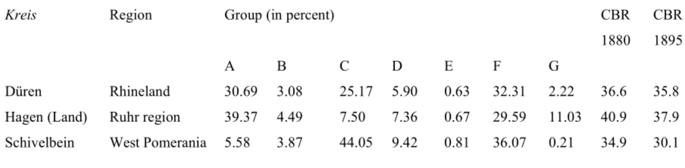
Table 3 provides three example districts. The variables A-G are the percentage of the working population in our seven insurance groups in 1882, and the CBRs are for reference. The treatment group A (industrial workers) accounts for 39 percent of the workforce in Hagen (Ruhr) in 1882. Group C (farm workers) are only 7.5 of this Ruhr Kreis. Düren has almost as many industrial workers (Group A) as Hagen, but more farm laborers (Group C) and fewer miners (Group G). Schivelbein, in Pomerania, has few industrial workers (Group A) or miners (Group G), but more farm laborers (Group C) than the other two Kreise. Model identification relies on these cross-sectional differences in treatment intensity in 1882.

Table 3: Treatment groups in three example districts

Kreis Region Group (in percent) CBR

1880

CBR 1895

A B C D E F G

Düren Rhineland 30.69 3.08 25.17 5.90 0.63 32.31 2.22 36.6 35.8

Hagen (Land) Ruhr region 39.37 4.49 7.50 7.36 0.67 29.59 11.03 40.9 37.9 Schivelbein West Pomerania 5.58 3.87 44.05 9.42 0.81 36.07 0.21 34.9 30.1

Using the time-period 1880 to 1895 gives us the immediate impact of each pillar, including the 1891 pension system. Our models have two sorts of “control groups:” the pre-program period for every Kreis as well as occupations that are not treated as of a specific year. Appendix C addresses the parallel pre-trends assumption. There we split the estimation sample into two groups defined by high and low values of the treatments A-G, and plot the trends in marriage and fertility for each group. There are no violations in the period we study.

Prior to Bismarck’s program, some Germans participated in voluntary schemes to insure against the vicissitudes of life. Private firms offered insurance plans, and some cities, employers, and civil-society

21

organizations offered insurance schemes. Contemporaries claimed that the new system crowded-out older schemes, but we know of no quantitative source documenting the extent of the issue.²⁴ Some people newly affected by the social-insurance scheme might have had earlier insurance that they dropped. For such persons our estimates reflect switching to the compulsory scheme, not insurance per se. The health- insurance system’s flexibility raises a related measurement problem. Our approach assumes that all health funds had the same policies during the initial years that we study.

One could reasonably ask when a given treatment began to influence demographic decisions.

Marriage and children reflect long-term commitments; when would individuals take a program as known and permanent, and make it the basis of decisions? Our reading of the political history reassures us that repealing or even scaling back the program was implausible. The more important question is when workers would begin to condition their behavior on the insurance system. Consider the health-insurance program.

Bismarck outlined his plan to establish a social security system in the German parliament (Reichstag) in 1881. Parliament passed the legislation in 1883, but the local health funds did not begin operation until 1884. A worker covered under this scheme might have adapted to it in 1881, when Bismarck announced the general plan (that is, there might be an “announcement effect”); in 1883, when parliament passed the law;

in 1884, when the health funds started operating; or perhaps later, after seeing the insurance plan in action.

The original accident-insurance law focused on industrial workers. The legislative debate over the system’s expansion in 1885 (that is, after the first round) reflects an agreement on extension to new groups of workers, but less agreement about which workers should be covered right away. There was no master plan for the three-stage roll-out. We think it unlikely that workers could have predicted the actual program history in 1881.²⁵

24 See, for example, Ludwig Bamberger’s warning to the Reichstag (Stenographische Berichte über die Verhandlungen des deutschen Reichstags, 4. Legislaturperiode, IV. Session 1881, Vol. 1, p. 675).

25 See, for example, the remarks by Julius Kräker, a Social Democrat, and the Liberal Karl Schrader (Stenographische Berichte über die Verhandlungen des deutschen Reichstags, 6. Legislaturperiode, I. Session 1881, Vol. 2, pp. 982-3 and 987).

22 Data

We construct the treatment variables from the distribution of worker occupations reported in the 1882 census of occupations.²⁶ The demographic variables (both the dependent variables and demographic controls) come from two sets of Prussian official data. The vital registration system reported events: births, deaths, marriages. Quinquennial population censuses report population sizes and urbanization for the period 1875 through 1910.²⁷ Ideally, our dependent variables would be age-standardized rates that take into account the population at risk of these events, but data limitations force us to rely on approximations. The marriage and fertility estimates pose slightly different challenges. For marriage, for example, we would like to know marital status by age. This level of detail is not available until 1890, and then only at five-year intervals.

Instead, we use the count of marriages celebrated as the dependent variable.

The sources provide separate counts of the number of legitimate and illegitimate births. Illegitimacy remained an important feature of Prussia demographic patterns into the twentieth century. While much lower than the levels observed in southern Germany, throughout our period the average Prussian Kreis saw 2-3 illegitimate births per thousand people each year. This figure varied dramatically across the country, with levels reaching eleven illegitimate births per thousand in some areas. Illegitimacy in Germany was the subject of considerable policy concern in our period, and a rich literature since has debated why it was elevated relative to other western European countries. One possible cause potentially affects our marriage estimates. Until the 1860s, many German states legally restricted marriage, often by requiring couples to obtain permission from local authorities after demonstrating their moral and economic fitness to be parents.

Not surprisingly, this politische Ehekonsens led many couples to have children without marrying. The restrictions were not as tough in “Old” Prussia as in the south German states, but some of Prussia’s 1866

26 Appendix B provides more detail on the data. We use the occupational census information as reported by the ifo Prussian Economic History Database (Becker et al, 2014).

27 These demographic variables all come from “Galloway Prussia Database 1861 to 1914. See Galloway (2007).

Galloway used as much detail as the sources reported.

23

territorial acquisitions had only repealed the Ehekonsens in the 1860s. A marriage boom in the 1870s reflects, in part, the end of these restrictions.²⁸

Because the insurance programs only provided benefits to illegitimate children if their mother was covered, in the fertility regressions our dependent variable is the count of legitimate births.²⁹ The accident insurance system might have promoted marriage because illegitimate children became legitimate when their parents married.³⁰ Thus the orphan benefits under the accident insurance system might have spurred some couples to marry after starting their families. If we combine legitimate and illegitimate births, the results change little. Appendix C reports results.

Econometric specifications

While we examined pooled models, we stress specifications that include Kreis and year fixed effects. The dependent variable is the natural log of a count. Our demographic controls include urbanization, population size, and the number of that population that is female. We cluster all standard errors at the level of the Kreis.

One of the demographic controls in the fertility equation is infant mortality. This control poses two challenges. First, with annual data, the mortality rates may in part convey information irrelevant to a decision about conception: many babies born in year t reflect conceptions in year t-1. Our regressions here ignore this issue, but robustness checks reported in Appendix C show that this simplification does not affect the

28 For evidence on the demographic implications of the politische Ehekonsens see Knodel (1967) or Guinnane and Ogilvie (2014). Ehmer (1991) provides more detail on the policy.

29 Galloway et al (1994) use the General Marital Fertility Rate (GMFR), which is the number of legitimate births to

married woman age 15-49. Theirs is the preferable measure, but to construct it requires two accommodations to the data. First, the denominator is only available in census years. Galloway et al thus construct a panel in which each cross- section reflects a census year; their dependent variable uses a five-year average of births, centered on the census year.

For our purposes, this approach would be wholly unsuitable, as we are interested in the year-to-year changes in fertility induced by the system’s introduction. Second, the Prussian sources do not report marital status by age until 1890, with the exception of large age bands reported as part of the occupational census of 1882, and do not report age-structure by sex after 1875. Galloway et al (1994) construct measures for the earlier period by applying the age-sex-marital status distributions of 1890 to the earlier population totals.

30 The same argument applies to local funds that extended health insurance to spouses and children. Prussian law (even

prior to the 1900 Civil Code) recognized the legitimation of children whose natural parents married (legitimation per matrimonium subsequens), provided the new husband declared himself the natural father (also filed a Vaterschaftanerkennung).

24

results. Second, we face the problem that infant mortality rates are endogenous to fertility. The literature discusses several channels. One channel would be unobserved heterogeneity; couples reluctant to use contraception might tolerate more child deaths. Other arguments stress the deleterious impact of a large (possibly closely-spaced) brood on child survival. Finding suitable instruments in this case is especially difficult, because most things that affect fertility also affect child survival. We focus on instruments that reflect the local disease environment.³¹ Many infants died because of exposure to pathogens before their immune systems were able to fight back. Infectious diseases spread via water and food contamination. We use the Kreis’s elevation in meters as one instrument. Diseases such as dysentery were worse at lower altitudes because of differences in temperature (especially summer temperatures).³² The elevation variable has no variation in the time dimension, but we interact it with year. The interaction captures the changing effect of elevation as public-health measures improved. Violation of the exclusion restriction would require that elevation affect fertility via channels other than mortality. One could imagine subtle differences in local economies at higher elevations that might affect fertility directly, but in a fixed-effects framework this is not a major concern. A second instrument, latitude, has a similar motivation. We use both instruments in our main specifications. They are individually and collectively “strong” but some specifications may not be over-identified. Just-identified models (using either instrument alone) produce similar results. Appendix C discusses the issue.

Studies of fertility and its decline usually employ additional controls for economic structure, religion, and culture, among other forces thought to affect fertility.³³ The models we report are in contrast relatively sparse for three considered reasons. First, some of these controls in other studies may not measure what the author intends. Galloway et al (1994), for example, use an “insurance” proxy that is the number of employees of insurance firms. They intend this as a proxy for reliance on financial instruments, a substitute

31 Schultz (1997, pp. 384-386) discusses this issue and provides additional references. If the issue really is unobserved heterogeneity, the FE specifications would suffice. See Brown (1988) for the improvement of public-health systems and Spree (1981) or Brown and Guinnane (2018) for infant and child mortality.

32 Malaria is also worse at lower altitudes. Until the middle of the nineteenth century, Prussia’s marshy areas supported malaria infestations. By the end of the century, Prussia had eliminated malaria, with the exception of some areas in the provinces of Schleswig-Holstein and Silesia. See Dalitz (2015, p. 2).

33 See Brown and Guinnane (2002), Galloway et al (1994) or Scheubel (2013) for examples using German data.

25

for children. At the Kreis level, this proxy surely indicates insurance company locations rather than the propensity to own insurance policies; Frankfurt has many insurance workers because many firms headquartered there, not because its people loved to buy insurance. Second, in a fixed-effects framework, such controls only matter to the extent they have year-to-year variation. Consider religion. Because few Prussians changed their religions, within-Kreis differences in religion largely reflect confessional differences in migration, fertility, or even mortality.³⁴ Cross-sectional differences in religion that do not change will be absorbed into the fixed effects. Finally, we study changes in marriage and legitimate fertility over a short time-span, periods over which there would be relatively little of the kind of structural or cultural change contemplated in the longer-term approach taken by others.

Results

The models include a large number of interaction terms. We find it simplest to interpret the results graphically and by reporting tests of linear restrictions. We begin with marriages for all of Prussia. Figure 6 displays the impacts and confidence intervals for groups A (industrial workers and white-collar workers), C (farm workers), and G (miners). (A and C are the two largest treated groups, while G serves as a control because these workers all had insurance prior to Bismarck. Appendix C presents results for Groups B, D, E, and F.) Recall that 1880 is the reference year for each treatment group. Thus the point-estimate for a given year tells us how much that group’s marriage or fertility behavior changed between 1880 and that year. We are more interested in the difference-in-difference: a comparison of the point-estimates for two different treatment groups in a single year. This difference-in-differences tells us how the different packages of social insurance affected the different groups.

34 Galloway et al (1994, note 64) refers to this issue. See Brown and Guinnane (2002) for additional discussion.

26

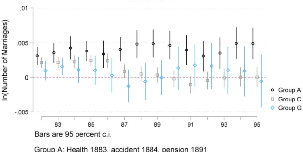
Figure 6: The effect of social insurance on marriage, all of Prussia

Note: The figure graphs the point-estimates and 95 percent confidence intervals for the regressions discussed in the text. Regression results are in Appendix C.

There were no changes in insurance status for Group G over this period, so it is reassuring that their marriage behavior did not change. Groups A and C are more complicated. The estimated effects are all small; the mean of the dependent variable is 6.28 (s.d. = .624) and the largest elasticity for any estimate in Figure 6 is .0016. The difference-in-difference for A and C in 1887 is statistically significant (p=0.0), but not for earlier years post-1884. This result might be consistent with a slow reaction to treatment by Group A: Group C’s first treatment was in 1887. Note that starting in 1888, there is a consistent (if small and statistically insignificant) decline in marriage rates for Group C. If this change reflects the program extension in 1887, this change marks a more rapid reaction than we see in other cases. The changes after 1891 are small relative to their standard errors, so we cannot conclude that the pension system affected marriage behavior.

27

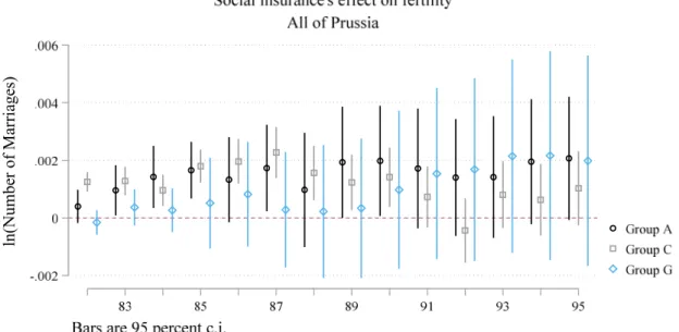
Figure 7: The effect of social insurance on fertility, all of Prussia

Note: The figure graphs the point-estimates and 95 percent confidence intervals for the regressions discussed in the text. Regression results are in Appendix C.

Figure 7 reports analogous results from the fertility model.³⁵ The estimates for A and G have large standard errors. For Group G, again, there is no effect from the programs, which is what we expect. For Group A the changes are small and come in the wrong years to tie to the social insurance program. The estimates for Group C are more complex. The difference-in-difference with Group A is never statistically significant, given the imprecise estimates for Group A. Once again, there is a downward trend in fertility for Group C; given our earlier results for marriage, this trend probably reflects reductions in marriage rather than control of marital fertility.

35The specification used here is IV with fixed effects. Appendix C reports and discusses the analogous model where we treat infant mortality as exogenous.

ln(Number of Marriages)

28

These models all have Kreis-level fixed effects that sweep out additive heterogeneity at that level.

But the model assumes common βs for different kinds of places. One might worry that the effect of a social insurance program’s introduction would differ between cities and rural areas, for example, or in different regions of Germany. Such differences could reflect information; in urban areas worker organizations might do a better job of publicizing the new programs and how to use them. The differences could also reflect differences in income level. Lehmann-Hasemeyer and Streb (2018) estimate the average annual income in eastern Prussia as about 91 percent of that in western Prussia.³⁶ A long historiography points out that the agricultural laborers who comprise Group C, and who were most numerous in the east, were especially poor.³⁷

We address these possible differences in two ways. First, we split the sample into Kreise that were primarily urban and those that were primarily rural. With few exceptions, even most urban areas were located in a Kreis that had considerable rural population. This makes it possible to keep all treatment groups in the same regression, but means there is no clean “urban vs rural” comparison possible. The results do not suggest important differences in this dimension and we relegate them to the appendix.

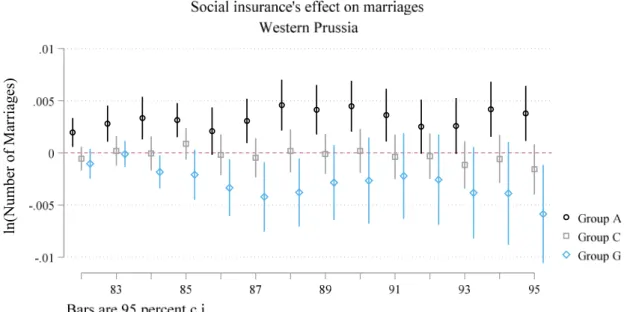
Our second approach resonates with an older historiography. Prussia’s eastern provinces differed considerably, both economically and socially, from her western provinces. One way these provinces differed was in their marriage patterns. Hajnal’s (1953, 1965) famous St. Petersburg-Trieste line puts all of Prussia on the side with the western European marriage pattern. But in eastern Prussia, people tended to marry much earlier and many more married than was the case in western Prussia or in other areas with the western European marriage pattern (Ehmer, 1991, pp. 103-111). We have argued that social insurance affected the incentives to marry, so it is natural to ask whether the program had a differential impact in the regions of Prussia. To construct Figures 8 and 9 we divided the Kreise into east and west. East is defined as in footnote

36 “Eastern” Prussia here means the Regierungsbezirke of Breslau, Bromberg, Danzig, Gumbinnen, Köslin,

Königsberg, Liegnitz, Marienwerder, Oppeln, Posen, Stettin and Stralsund. Cinnirella and Streb (2017) show that eastern Prussia was also less innovative (as measured by patenting activity) than the western part of the country.

37 Many of these farm workers were of Polish nationality. Wolf et al (2019) observe that differences in the distribution of Germans and Poles explain differences in income levels, savings and literacy rates at the Kreis level in eastern Prussia. Nationality might have affected marriage rates and fertility, as well.

29

36, but dividing at median longitude does not generate appreciably different results. The upper panel of Figure 8 reports results for marriage for western and central Prussia. These results look much like the results for Prussia as a whole (Figure 6). The lower panel tells a different story for the eastern provinces, however.

The movements for Group G are disconcerting, since it was not treated in this period. But something happened to Group C, the farm workers, after their 1886 treatment. The difference-in-difference of A versus C in 1887 is significant (p=.028) as is C in 1886 compared to 1887 (p=.025). It seems that farm workers became more attractive husbands after they were covered by the accident insurance with their generous pensions. Figure 9 reports a similar set of exercises for fertility. Here we see essentially no effects at all.

Figure 8: The effect of social insurance on marriage in western and eastern Prussia

ln(Number of Marriages)

30

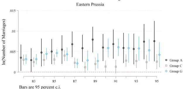
Figure 9: The effect of social insurance on fertility in western and eastern Prussia

ln(Number of Marriages)ln(Number of Marriages)

31

Note: The figure graphs the point-estimates and 95 percent confidence intervals for the regressions discussed in the text. Regression results are in Appendix C.

Conclusions

Bismarck’s famous social insurance system came into being at the start of Germany’s fertility transition. Economic theories of fertility would argue that this is not pure coincidence: if couples have children in part to provide insurance against old age and infirmity, we would expect state-supported assistance to induce couples to have fewer children. Following this logic, some observers today ascribe low fertility in wealthy countries to the effect of social insurance.

Did Bismarck’s program play a role in the fertility transition? Earlier research that focuses on the 1891 pension system argues that it did. In this paper, we approach the problem differently. As we stress, the first two pillars of the social insurance system, health and accident insurance, were much more generous than the 1891 old age pension and also had elements that plausibly affected marriage and fertility. This argues for considering each of the three distinct programs and for considering their effect on each other. Our

ln(Number of Marriages)

32

difference-in-difference approach uses the distribution of covered occupations to infer the intensity of treatment for each of about Prussian 450 districts. We also analyze the effect on marriages and fertility separately. At this stage in the fertility transition, marriage remained a primary regulator of fertility, and the social insurance system’s incentives related to marriage were considerable.

Our results may reflect the limitations of the data available to us. Lacking any individual-level data, we have to rely on aggregates that may mask changes. However, our findings should give pause to those who want to blame the welfare state for low fertility. At the start of the fertility transition, a generous and compulsory social insurance scheme did not have noticeable effects on marriage or fertility.